chapter 8: using the discrete ordinates radiation...
TRANSCRIPT
Chapter 8: Using the Discrete Ordinates Radiation Model
This tutorial is divided into the following sections:
8.1. Introduction
8.2. Prerequisites
8.3. Problem Description
8.4. Setup and Solution
8.5. Summary
8.6. Further Improvements
8.1. Introduction
This tutorial illustrates the set up and solution of flow and thermal modelling of a headlamp. The discrete
ordinates (DO) radiation model will be used to model the radiation.
This tutorial demonstrates how to do the following:
• Read an existing mesh file into ANSYS FLUENT.
• Set up the DO radiation model.
• Set up material properties and boundary conditions.
• Solve for the energy and flow equations.
• Initialize and obtain a solution.
• Postprocess the resulting data.
• Understand the effect of pixels and divisions on temperature predictions and solver speed.
8.2. Prerequisites
This tutorial is written with the assumption that you have completed one or more of the introductory
tutorials found in this manual:
• Introduction to Using ANSYS FLUENT in ANSYS Workbench: Fluid Flow and Heat Transfer in a Mixing
Elbow (p. 1)
• Parametric Analysis in ANSYS Workbench Using ANSYS FLUENT (p. 77)
• Introduction to Using ANSYS FLUENT: Fluid Flow and Heat Transfer in a Mixing Elbow (p. 131)
and that you are familiar with the ANSYS FLUENT navigation pane and menu structure. Some steps in
the setup and solution procedure will not be shown explicitly.
8.3. Problem Description
The problem to be considered is illustrated in Figure 8.1 (p. 360), showing a simple two-dimensional
section of a headlamp construction. The key components to be included are the bulb, reflector, baffle,
lens, and housing. For simplicity, the heat output will only be considered from the bulb surface rather
359Release 14.0 - © SAS IP, Inc. All rights reserved. - Contains proprietary and confidential information
of ANSYS, Inc. and its subsidiaries and affiliates.

than the filament of the bulb. The radiant load from the bulb will cover all thermal radiation - this includes
visible (light) as well as infrared radiation.
The ambient conditions to be considered are quiescent air at 20°C. Heat exchange between the lamp
and the surroundings will occur by conduction, convection and radiation. The rear reflector is assumed
to be well insulated and heat losses will be ignored. The purpose of the baffle is to shield the lens from
direct radiation. Both the reflector and baffle are made from polished metal having a low emissivity
and mirror-like finish; their combined effect should distribute the light and heat from the bulb across
the lens. The lens is made from glass and has a refractive index of 1.5.
Figure 8.1 Schematic of the Problem
8.4. Setup and Solution
The following sections describe the setup and solution steps for this tutorial:
8.4.1. Preparation
8.4.2. Step 1: Mesh
8.4.3. Step 2: General Settings
8.4.4. Step 3: Models
8.4.5. Step 4: Materials
8.4.6. Step 5: Cell Zone Conditions
8.4.7. Step 6: Boundary Conditions
8.4.8. Step 7: Solution
8.4.9. Step 8: Postprocessing
8.4.10. Step 9: Iterate for Higher Pixels
8.4.11. Step 10: Iterate for Higher Divisions
8.4.12. Step 11: Make the Reflector Completely Diffuse
8.4.13. Step 12: Change the Boundary Type of Baffle
Release 14.0 - © SAS IP, Inc. All rights reserved. - Contains proprietary and confidential informationof ANSYS, Inc. and its subsidiaries and affiliates.360
Chapter 8: Using the Discrete Ordinates Radiation Model
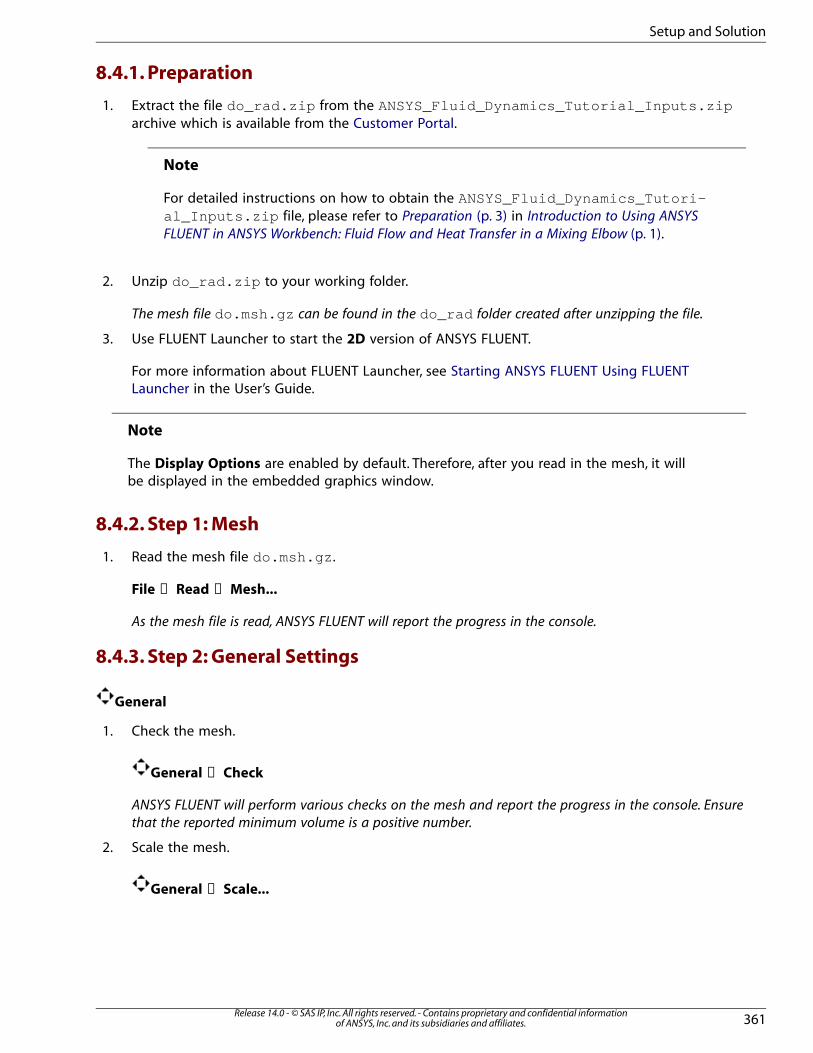
8.4.1. Preparation
1. Extract the file do_rad.zip from the ANSYS_Fluid_Dynamics_Tutorial_Inputs.ziparchive which is available from the Customer Portal.
Note
For detailed instructions on how to obtain the ANSYS_Fluid_Dynamics_Tutori-al_Inputs.zip file, please refer to Preparation (p. 3) in Introduction to Using ANSYS
FLUENT in ANSYS Workbench: Fluid Flow and Heat Transfer in a Mixing Elbow (p. 1).
2. Unzip do_rad.zip to your working folder.
The mesh file do.msh.gz can be found in the do_rad folder created after unzipping the file.
3. Use FLUENT Launcher to start the 2D version of ANSYS FLUENT.
For more information about FLUENT Launcher, see Starting ANSYS FLUENT Using FLUENT
Launcher in the User’s Guide.
Note
The Display Options are enabled by default. Therefore, after you read in the mesh, it will
be displayed in the embedded graphics window.
8.4.2. Step 1: Mesh
1. Read the mesh file do.msh.gz .
File → Read → Mesh...
As the mesh file is read, ANSYS FLUENT will report the progress in the console.
8.4.3. Step 2: General Settings
General
1. Check the mesh.
General → Check
ANSYS FLUENT will perform various checks on the mesh and report the progress in the console. Ensure
that the reported minimum volume is a positive number.
2. Scale the mesh.
General → Scale...
361Release 14.0 - © SAS IP, Inc. All rights reserved. - Contains proprietary and confidential information
of ANSYS, Inc. and its subsidiaries and affiliates.
Setup and Solution
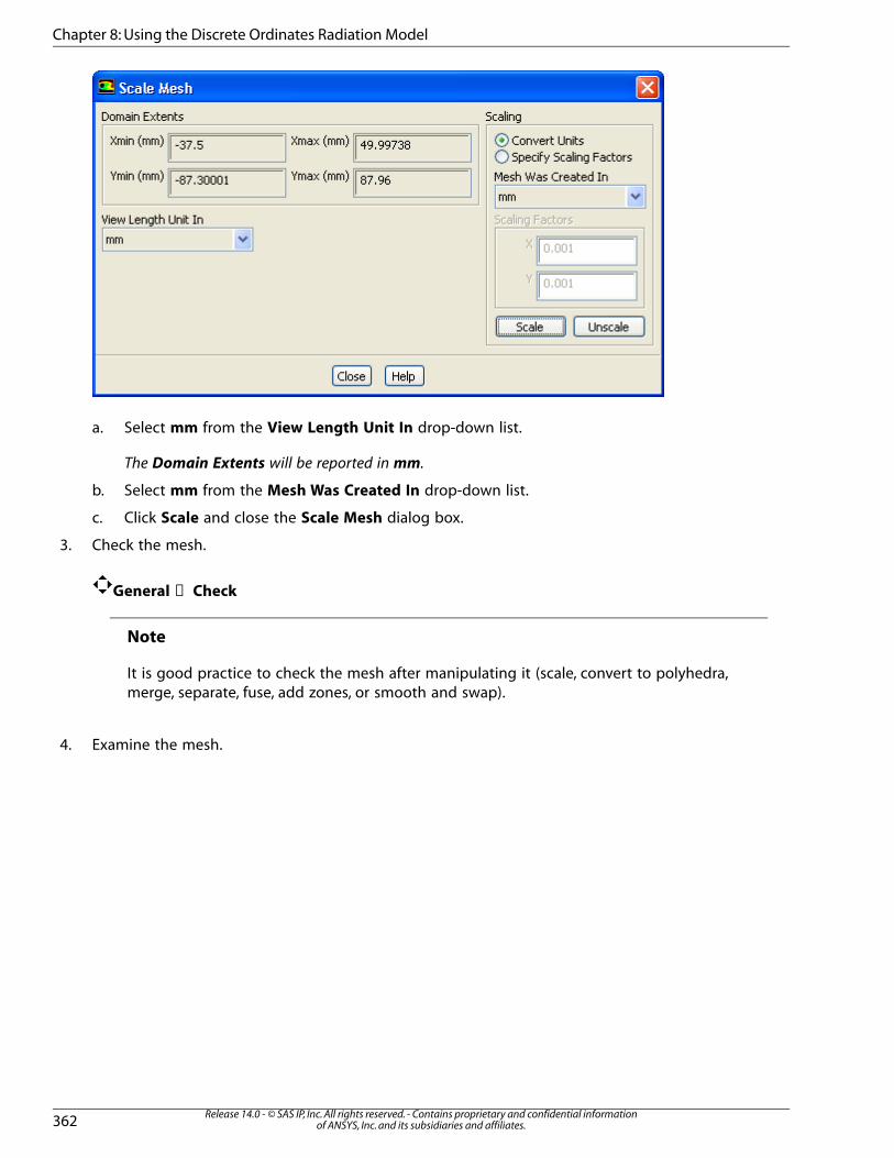
a. Select mm from the View Length Unit In drop-down list.
The Domain Extents will be reported in mm.
b. Select mm from the Mesh Was Created In drop-down list.
c. Click Scale and close the Scale Mesh dialog box.
3. Check the mesh.
General → Check
Note
It is good practice to check the mesh after manipulating it (scale, convert to polyhedra,
merge, separate, fuse, add zones, or smooth and swap).
4. Examine the mesh.
Release 14.0 - © SAS IP, Inc. All rights reserved. - Contains proprietary and confidential informationof ANSYS, Inc. and its subsidiaries and affiliates.362
Chapter 8: Using the Discrete Ordinates Radiation Model

Figure 8.2 Graphics Display of Mesh
5. Change the unit of temperature to centigrade.
General → Units...
363Release 14.0 - © SAS IP, Inc. All rights reserved. - Contains proprietary and confidential information
of ANSYS, Inc. and its subsidiaries and affiliates.
Setup and Solution
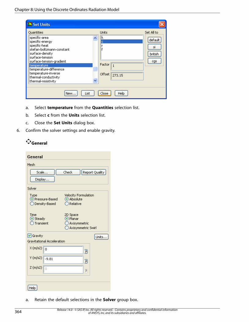
a. Select temperature from the Quantities selection list.
b. Select c from the Units selection list.
c. Close the Set Units dialog box.
6. Confirm the solver settings and enable gravity.
General
a. Retain the default selections in the Solver group box.
Release 14.0 - © SAS IP, Inc. All rights reserved. - Contains proprietary and confidential informationof ANSYS, Inc. and its subsidiaries and affiliates.364
Chapter 8: Using the Discrete Ordinates Radiation Model

b. Enable Gravity.
c. Enter -9.81 � �� for Gravitational Acceleration in the Y direction.
8.4.4. Step 3: Models
Models
1. Enable the energy equation.
Models → Energy → Edit...
2. Enable the DO radiation model.
Models → Radiation → Edit...
a. Select Discrete Ordinates (DO) in the Model list.
The Radiation Model dialog box expands to show the related inputs.
b. Set the Flow Iterations per Radiation Iteration to 1.
As radiation will be the dominant mode of heat transfer, it is beneficial to reduce the interval
between calculations. For this small 2D case we will reduce it to 1.
c. Retain the default settings for Angular Discretization.
d. Click OK to close the Radiation Model dialog box.
365Release 14.0 - © SAS IP, Inc. All rights reserved. - Contains proprietary and confidential information
of ANSYS, Inc. and its subsidiaries and affiliates.
Setup and Solution

An Information dialog box will appear, indicating that material properties have changed.
e. Click OK in the Information dialog box.
8.4.5. Step 4: Materials
Materials
1. Set the properties for air.
Materials → air → Create/Edit...
a. Select incompressible-ideal-gas from the Density drop-down list.
Since pressure variations are insignificant compared to temperature variation, we choose incom-
pressible-ideal-gas law for density.
b. Retain the default settings for all other parameters.
c. Click Change/Create and close the Create/Edit Materials dialog box.
2. Create a new material, lens.
Release 14.0 - © SAS IP, Inc. All rights reserved. - Contains proprietary and confidential informationof ANSYS, Inc. and its subsidiaries and affiliates.366
Chapter 8: Using the Discrete Ordinates Radiation Model

Materials → Solid → Create/Edit...
a. Enter lens for Name and delete the entry in the Chemical Formula field.
b. Enter 2200 �� �� for Density.
c. Enter 830 J/Kg-K for Cp (Specific Heat).
d. Enter 1.5 W/m-K for Thermal Conductivity.
e. Enter 200 1/m for Absorption Coefficient.
f. Enter 1.5 for Refractive Index.
g. Click Change/Create.
A Question dialog box will open, asking if you want to overwrite aluminum.
h. Click No in the Question dialog box to retain aluminum and add the new material (lens) to the
materials list.
The Create/Edit Materials dialog box will be updated to show the new material, lens, in the
ANSYS FLUENT Solid Materials drop-down list.
i. Close the Create/Edit Materials dialog box.
367Release 14.0 - © SAS IP, Inc. All rights reserved. - Contains proprietary and confidential information
of ANSYS, Inc. and its subsidiaries and affiliates.
Setup and Solution

8.4.6. Step 5: Cell Zone Conditions
Cell Zone Conditions
1. Ensure that air is selected for fluid.
Cell Zone Conditions → fluid → Edit...
Release 14.0 - © SAS IP, Inc. All rights reserved. - Contains proprietary and confidential informationof ANSYS, Inc. and its subsidiaries and affiliates.368
Chapter 8: Using the Discrete Ordinates Radiation Model
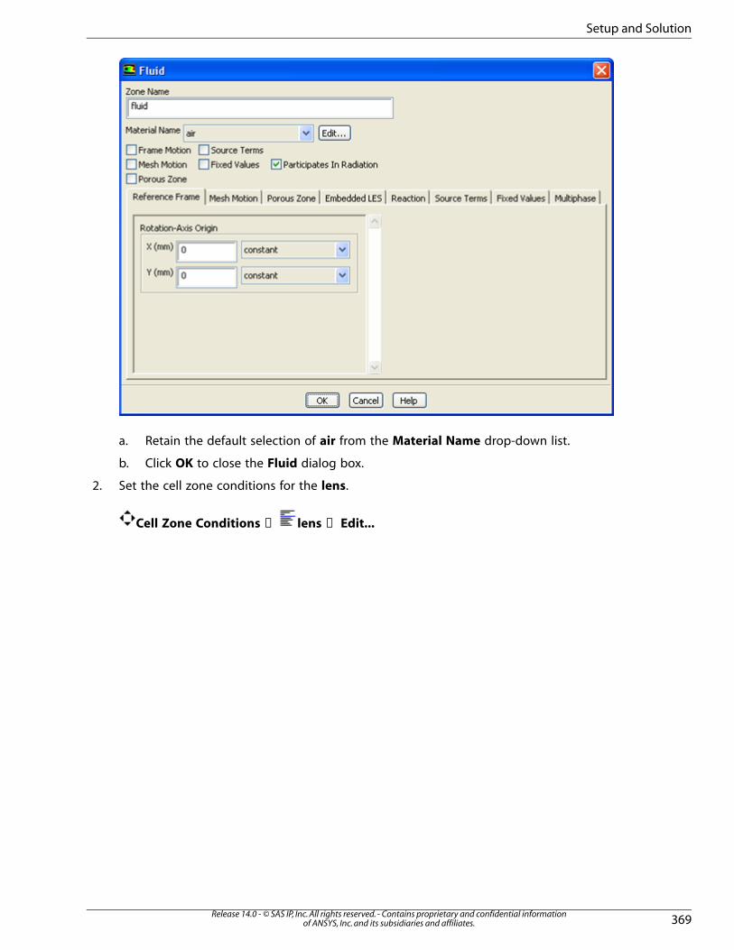
a. Retain the default selection of air from the Material Name drop-down list.
b. Click OK to close the Fluid dialog box.
2. Set the cell zone conditions for the lens.
Cell Zone Conditions → lens → Edit...
369Release 14.0 - © SAS IP, Inc. All rights reserved. - Contains proprietary and confidential information
of ANSYS, Inc. and its subsidiaries and affiliates.
Setup and Solution

a. Select lens from the Material Name drop-down list.
b. Enable Participates In Radiation.
c. Click OK to close the Solid dialog box.
8.4.7. Step 6: Boundary Conditions
Boundary Conditions
Release 14.0 - © SAS IP, Inc. All rights reserved. - Contains proprietary and confidential informationof ANSYS, Inc. and its subsidiaries and affiliates.370
Chapter 8: Using the Discrete Ordinates Radiation Model

1. Set the boundary conditions for the baffle.
Boundary Conditions → baffle → Edit...
371Release 14.0 - © SAS IP, Inc. All rights reserved. - Contains proprietary and confidential information
of ANSYS, Inc. and its subsidiaries and affiliates.
Setup and Solution

a. Click the Thermal tab and enter 0.1 for Internal Emissivity.
b. Click the Radiation tab and enter 0 for Diffuse Fraction.
c. Click OK to close the Wall dialog box.
2. Set the boundary conditions for the baffle-shadow.
Boundary Conditions → baffle-shadow → Edit...
Release 14.0 - © SAS IP, Inc. All rights reserved. - Contains proprietary and confidential informationof ANSYS, Inc. and its subsidiaries and affiliates.372
Chapter 8: Using the Discrete Ordinates Radiation Model
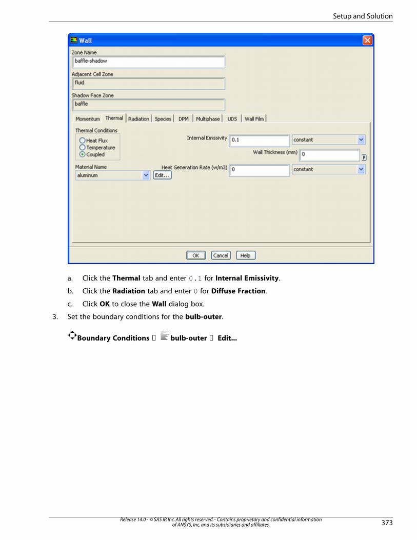
a. Click the Thermal tab and enter 0.1 for Internal Emissivity.
b. Click the Radiation tab and enter 0 for Diffuse Fraction.
c. Click OK to close the Wall dialog box.
3. Set the boundary conditions for the bulb-outer.
Boundary Conditions → bulb-outer → Edit...
373Release 14.0 - © SAS IP, Inc. All rights reserved. - Contains proprietary and confidential information
of ANSYS, Inc. and its subsidiaries and affiliates.
Setup and Solution

a. Click the Thermal tab and enter 150000 � �� for Heat Flux.
The circumference of bulb-outer is approximately �. Therefore the �� lineal heat
flux specified in the problem description corresponds to ���.
b. Retain the value of 1 for Internal Emissivity.
c. Click OK to close the Wall dialog box.
4. Set the boundary conditions for the housing.
Boundary Conditions → housing → Edit...
Release 14.0 - © SAS IP, Inc. All rights reserved. - Contains proprietary and confidential informationof ANSYS, Inc. and its subsidiaries and affiliates.374
Chapter 8: Using the Discrete Ordinates Radiation Model
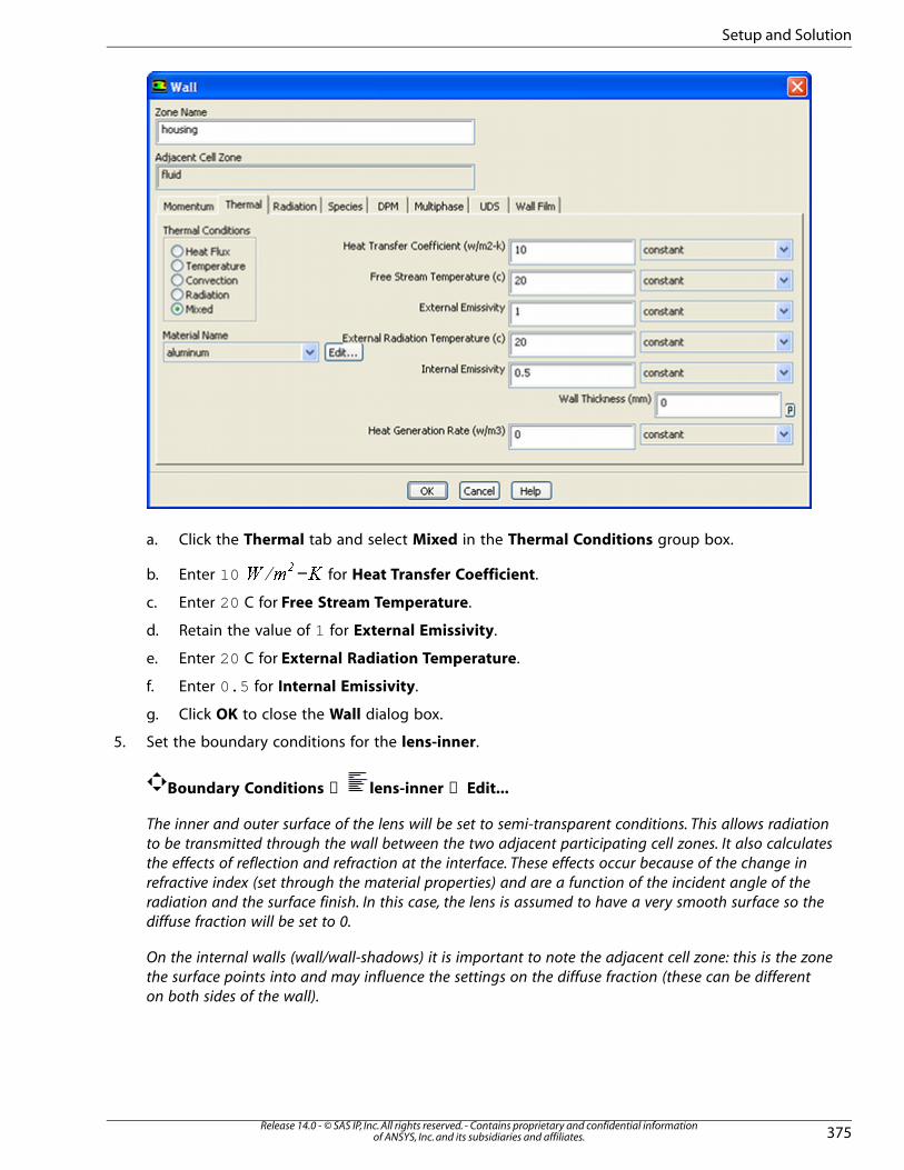
a. Click the Thermal tab and select Mixed in the Thermal Conditions group box.
b. Enter 10 −� � ��
for Heat Transfer Coefficient.
c. Enter 20 C for Free Stream Temperature.
d. Retain the value of 1 for External Emissivity.
e. Enter 20 C for External Radiation Temperature.
f. Enter 0.5 for Internal Emissivity.
g. Click OK to close the Wall dialog box.
5. Set the boundary conditions for the lens-inner.
Boundary Conditions → lens-inner → Edit...
The inner and outer surface of the lens will be set to semi-transparent conditions. This allows radiation
to be transmitted through the wall between the two adjacent participating cell zones. It also calculates
the effects of reflection and refraction at the interface. These effects occur because of the change in
refractive index (set through the material properties) and are a function of the incident angle of the
radiation and the surface finish. In this case, the lens is assumed to have a very smooth surface so the
diffuse fraction will be set to 0.
On the internal walls (wall/wall-shadows) it is important to note the adjacent cell zone: this is the zone
the surface points into and may influence the settings on the diffuse fraction (these can be different
on both sides of the wall).
375Release 14.0 - © SAS IP, Inc. All rights reserved. - Contains proprietary and confidential information
of ANSYS, Inc. and its subsidiaries and affiliates.
Setup and Solution

a. Click the Radiation tab.
b. Select semi-transparent from the BC Type drop-down list.
c. Enter 0 for Diffuse Fraction.
d. Click OK to close the Wall dialog box.
6. Set the boundary conditions for the lens-inner-shadow.
Boundary Conditions → lens-inner-shadow → Edit...
a. Click the Radiation tab.
b. Retain the default selection of semi-transparent from the BC Type drop-down list.
c. Enter 0 for Diffuse Fraction.
d. Click OK to close the Wall dialog box.
7. Set the boundary conditions for the lens-outer.
Boundary Conditions → lens-outer → Edit...
The surface of the lamp cools mainly by natural convection to the surroundings. As the outer lens is
transparent it must also lose radiation to the surroundings, while the surroundings will supply a small
source of background radiation associated with the temperature. For the lens, a semi-transparent
condition is used on the outside wall. A mixed thermal condition provides the source of background
radiation as well as calculating the convective cooling on the outer lens wall. For a semi-transparent
wall, the source of background radiation is added directly to the DO radiation rather than to the energy
Release 14.0 - © SAS IP, Inc. All rights reserved. - Contains proprietary and confidential informationof ANSYS, Inc. and its subsidiaries and affiliates.376
Chapter 8: Using the Discrete Ordinates Radiation Model
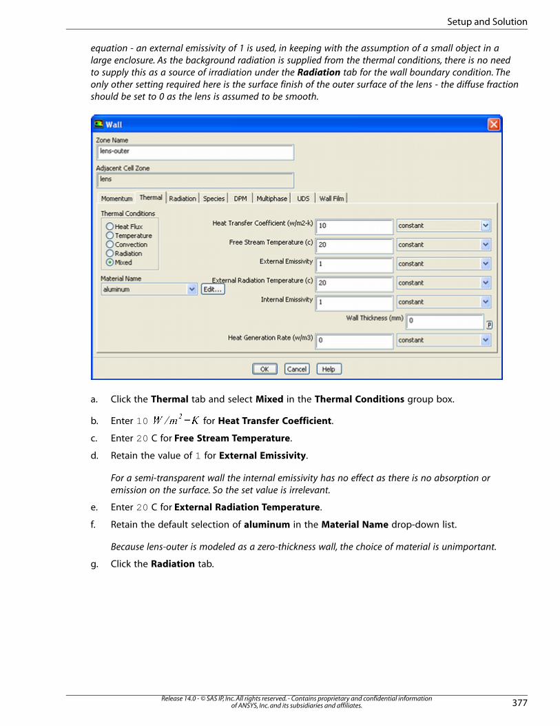
equation - an external emissivity of 1 is used, in keeping with the assumption of a small object in a
large enclosure. As the background radiation is supplied from the thermal conditions, there is no need
to supply this as a source of irradiation under the Radiation tab for the wall boundary condition. The
only other setting required here is the surface finish of the outer surface of the lens - the diffuse fraction
should be set to 0 as the lens is assumed to be smooth.
a. Click the Thermal tab and select Mixed in the Thermal Conditions group box.
b. Enter 10 −� � ��
for Heat Transfer Coefficient.
c. Enter 20 C for Free Stream Temperature.
d. Retain the value of 1 for External Emissivity.
For a semi-transparent wall the internal emissivity has no effect as there is no absorption or
emission on the surface. So the set value is irrelevant.
e. Enter 20 C for External Radiation Temperature.
f. Retain the default selection of aluminum in the Material Name drop-down list.
Because lens-outer is modeled as a zero-thickness wall, the choice of material is unimportant.
g. Click the Radiation tab.
377Release 14.0 - © SAS IP, Inc. All rights reserved. - Contains proprietary and confidential information
of ANSYS, Inc. and its subsidiaries and affiliates.
Setup and Solution

h. Select semi-transparent from the BC Type drop-down list.
i. Enter 0 for Diffuse Fraction.
j. Click OK to close the Wall dialog box.
8. Set the boundary conditions for the reflector.
Boundary Conditions → reflector → Edit...
Like the baffles, the reflector is made of highly polished aluminum, giving it highly reflective surface
property. About 90% of incident radiation reflects from this surface. Only 10% gets absorbed. Based
on Kirchhoff’s law, we can assume emissivity equals absorptivity. Therefore, we apply internal
emissivity = 0.1. We also assume a clean reflector (diffuse fraction = 0).
a. Click the Thermal tab and enter 0.1 for Internal Emissivity.
b. Click the Radiation tab and enter 0 for Diffuse Fraction.
c. Click OK to close the Wall dialog box.
8.4.8. Step 7: Solution
1. Set the solution parameters.
Solution Methods
Release 14.0 - © SAS IP, Inc. All rights reserved. - Contains proprietary and confidential informationof ANSYS, Inc. and its subsidiaries and affiliates.378
Chapter 8: Using the Discrete Ordinates Radiation Model

a. Select Body Force Weighted from the Pressure drop-down list in the Spatial Discretizationgroup box.
2. Set the under-relaxation factors.
Solution Controls
379Release 14.0 - © SAS IP, Inc. All rights reserved. - Contains proprietary and confidential information
of ANSYS, Inc. and its subsidiaries and affiliates.
Setup and Solution

a. Enter 0.7 for Pressure.
b. Enter 0.6 for Momentum.
3. Reduce the convergence criteria.
Monitors → Residuals → Edit...
a. Enter 1e-4 for Absolute Criteria for continuity.
Release 14.0 - © SAS IP, Inc. All rights reserved. - Contains proprietary and confidential informationof ANSYS, Inc. and its subsidiaries and affiliates.380
Chapter 8: Using the Discrete Ordinates Radiation Model
b. Ensure that Print to Console and Plot are enabled.
c. Click OK to close the Residual Monitors dialog box.
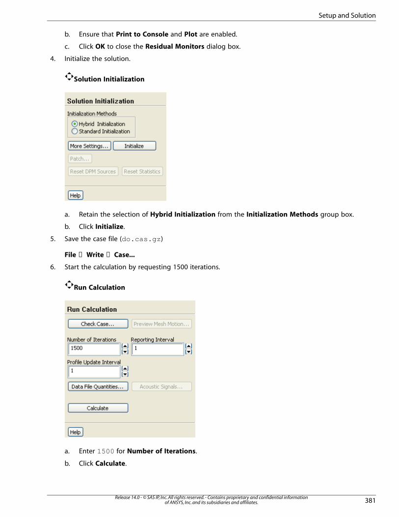
4. Initialize the solution.
Solution Initialization
a. Retain the selection of Hybrid Initialization from the Initialization Methods group box.
b. Click Initialize.
5. Save the case file (do.cas.gz )
File → Write → Case...
6. Start the calculation by requesting 1500 iterations.
Run Calculation
a. Enter 1500 for Number of Iterations.
b. Click Calculate.
381Release 14.0 - © SAS IP, Inc. All rights reserved. - Contains proprietary and confidential information
of ANSYS, Inc. and its subsidiaries and affiliates.
Setup and Solution

Figure 8.3 Residuals
The solution will converge in approximately 1020 iterations.
7. Save the case and data files (do.cas.gz and do.dat.gz ).
File → Write → Case & Data...
8.4.9. Step 8: Postprocessing
1. Display velocity vectors.
Graphics and Animations → Vectors → Set Up...
Release 14.0 - © SAS IP, Inc. All rights reserved. - Contains proprietary and confidential informationof ANSYS, Inc. and its subsidiaries and affiliates.382
Chapter 8: Using the Discrete Ordinates Radiation Model

a. Enter 10 for Scale.
b. Retain the default selection of Velocity from the Vectors of drop-down list.
c. Retain the default selection of Velocity... and Velocity Magnitude from the Color by drop-down
list.
d. Click Display (Figure 8.4 (p. 384)).
e. Close the Vectors dialog box.
383Release 14.0 - © SAS IP, Inc. All rights reserved. - Contains proprietary and confidential information
of ANSYS, Inc. and its subsidiaries and affiliates.
Setup and Solution

Figure 8.4 Vectors of Velocity Magnitude
2. Create the new surface, lens.
Surface → Zone...
Release 14.0 - © SAS IP, Inc. All rights reserved. - Contains proprietary and confidential informationof ANSYS, Inc. and its subsidiaries and affiliates.384
Chapter 8: Using the Discrete Ordinates Radiation Model

a. Select lens from the Zone selection list.
b. Click Create and close the Zone Surface dialog box.
3. Display contours of static temperature.
Graphics and Animations → Contours → Set Up...
a. Enable Filled in the Options group box.
b. Disable Global Range in the Options group box.
c. Select Temperature... and Static Temperature from the Contours of drop-down lists.
385Release 14.0 - © SAS IP, Inc. All rights reserved. - Contains proprietary and confidential information
of ANSYS, Inc. and its subsidiaries and affiliates.
Setup and Solution
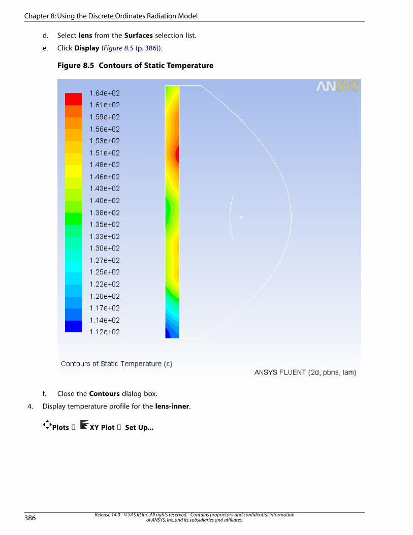
d. Select lens from the Surfaces selection list.
e. Click Display (Figure 8.5 (p. 386)).
Figure 8.5 Contours of Static Temperature
f. Close the Contours dialog box.
4. Display temperature profile for the lens-inner.
Plots → XY Plot → Set Up...
Release 14.0 - © SAS IP, Inc. All rights reserved. - Contains proprietary and confidential informationof ANSYS, Inc. and its subsidiaries and affiliates.386
Chapter 8: Using the Discrete Ordinates Radiation Model

a. Disable both Node Values and Position on X Axis in the Options group box.
b. Enable Position on Y Axis.
c. Enter 0 and 1 for X and Y, respectively, in the Plot Direction group box.
d. Retain the default selection of Direction Vector from the Y Axis Function drop-down list.
e. Select Temperature... and Wall Temperature (Outer Surface) from the X Axis Function drop-
down lists.
f. Select lens-inner from the Surfaces selection list.
g. Click the Axes... button to open the Axes - Solution XY Plot dialog box.
i. Ensure that X is selected in the Axis list.
387Release 14.0 - © SAS IP, Inc. All rights reserved. - Contains proprietary and confidential information
of ANSYS, Inc. and its subsidiaries and affiliates.
Setup and Solution

ii. Enter Temperature on Lens Inner for Label.
iii. Select float from the Type drop-down list in the Number Format group box.
iv. Set Precision to 0.
v. Click Apply.
vi. Select Y in the Axis list.
vii. Enter Y Position on Lens Inner for Label.
viii. Select float from the Type drop-down list in the Number Format group box.
ix. Set Precision to 0.
x. Click Apply and close the Axes - Solution XY Plot dialog box.
h. Click the Curves... button to open the Curves - Solution XY Plot dialog box.
i. Select the line pattern as shown in the Curves - Solution XY Plot dialog box.
ii. Select the symbol pattern as shown in the Curves - Solution XY Plot dialog box.
iii. Click Apply and close the Curves - Solution XY Plot dialog box.
Release 14.0 - © SAS IP, Inc. All rights reserved. - Contains proprietary and confidential informationof ANSYS, Inc. and its subsidiaries and affiliates.388
Chapter 8: Using the Discrete Ordinates Radiation Model

i. Click Plot (Figure 8.6 (p. 389)).
Figure 8.6 Temperature Profile for lens-inner
j. Enable Write to File and click the Write... button to open the Select File dialog box.
i. Enter do_2x2_1x1.xy for XY File.
ii. Click OK to close the Select File dialog box.
k. Close the Solution XY Plot dialog box.
8.4.10. Step 9: Iterate for Higher Pixels
1. Increase pixelation for accuracy.
Models → Radiation → Edit...
For semi-transparent and reflective surfaces, increasing accuracy by increasing pixilation is more efficient
than increasing theta and phi divisions.
389Release 14.0 - © SAS IP, Inc. All rights reserved. - Contains proprietary and confidential information
of ANSYS, Inc. and its subsidiaries and affiliates.
Setup and Solution
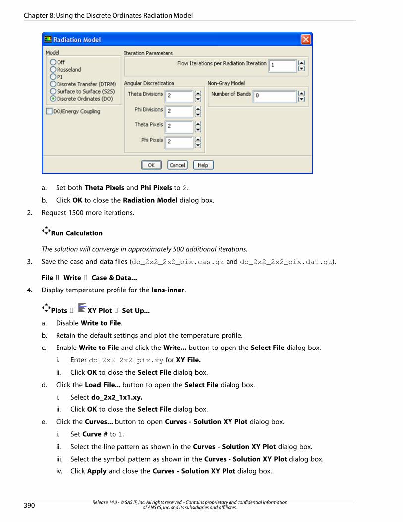
a. Set both Theta Pixels and Phi Pixels to 2.
b. Click OK to close the Radiation Model dialog box.
2. Request 1500 more iterations.
Run Calculation
The solution will converge in approximately 500 additional iterations.
3. Save the case and data files (do_2x2_2x2_pix.cas.gz and do_2x2_2x2_pix.dat.gz ).
File → Write → Case & Data...
4. Display temperature profile for the lens-inner.
Plots → XY Plot → Set Up...
a. Disable Write to File.
b. Retain the default settings and plot the temperature profile.
c. Enable Write to File and click the Write... button to open the Select File dialog box.
i. Enter do_2x2_2x2_pix.xy for XY File.
ii. Click OK to close the Select File dialog box.
d. Click the Load File... button to open the Select File dialog box.
i. Select do_2x2_1x1.xy.
ii. Click OK to close the Select File dialog box.
e. Click the Curves... button to open Curves - Solution XY Plot dialog box.
i. Set Curve # to 1.
ii. Select the line pattern as shown in the Curves - Solution XY Plot dialog box.
iii. Select the symbol pattern as shown in the Curves - Solution XY Plot dialog box.
iv. Click Apply and close the Curves - Solution XY Plot dialog box.
Release 14.0 - © SAS IP, Inc. All rights reserved. - Contains proprietary and confidential informationof ANSYS, Inc. and its subsidiaries and affiliates.390
Chapter 8: Using the Discrete Ordinates Radiation Model

f. Disable Write to File.
g. Click Plot (Figure 8.7 (p. 391)).
Figure 8.7 Temperature Profile for lens-inner
h. Close the Solution XY Plot dialog box.
5. Increase both Theta Pixels and Phi Pixels to 3 and continue iterations.
Models → Radiation → Edit...
6. Click the Calculate button.
Run Calculation
391Release 14.0 - © SAS IP, Inc. All rights reserved. - Contains proprietary and confidential information
of ANSYS, Inc. and its subsidiaries and affiliates.
Setup and Solution

The solution will converge in approximately 400 additional iterations.
7. Save the case and data files (do_2x2_3x3_pix.cas.gz and do_2x2_3x3_pix.dat.gz ).
File → Write → Case & Data...
8. Display temperature profile for the lens-inner.
Plots → XY Plot → Set Up...
a. Make sure Write to File is disabled.
b. Ensure that all files are deselected from the File Data selection list.
c. Ensure that lens-inner is selected from the Surfaces selection list.
d. Click Plot.
e. Click Write to File and save the file as do_2x2_3x3_pix.xy .
9. Repeat the procedure for 10 Theta Pixels and Phi Pixels and save the case and data files
(do_2x2_10x10_pix.cas.gz and do_2x2_10x10_pix.dat.gz ).
a. Save the file as do_2x2_10x10_pix.xy .
10. Read in all the files and plot them.
Plots → XY Plot → Set Up...
a. Click the Load File... button to open the Select File dialog box.
i. Select all the xy files and close the Select File dialog box.
Note
Selected files will be listed in the XY File(s) selection list.
Make sure you deselect lens-inner from the Surfaces list so that there is no duplicated plot.
b. Click the Curves... button to open Curves - Solution XY Plot dialog box.
i. Select the line pattern as shown in the Curves - Solution XY Plot dialog box.
ii. Select the symbol pattern as shown in the Curves - Solution XY Plot dialog box.
iii. Click Apply to save the settings for curve zero.
Release 14.0 - © SAS IP, Inc. All rights reserved. - Contains proprietary and confidential informationof ANSYS, Inc. and its subsidiaries and affiliates.392
Chapter 8: Using the Discrete Ordinates Radiation Model
iv. Set Curve # to 1.
v. Follow the above instructions for curves 2, 3, and 4.
vi. Click Apply and close the Curves - Solution XY Plot dialog box.
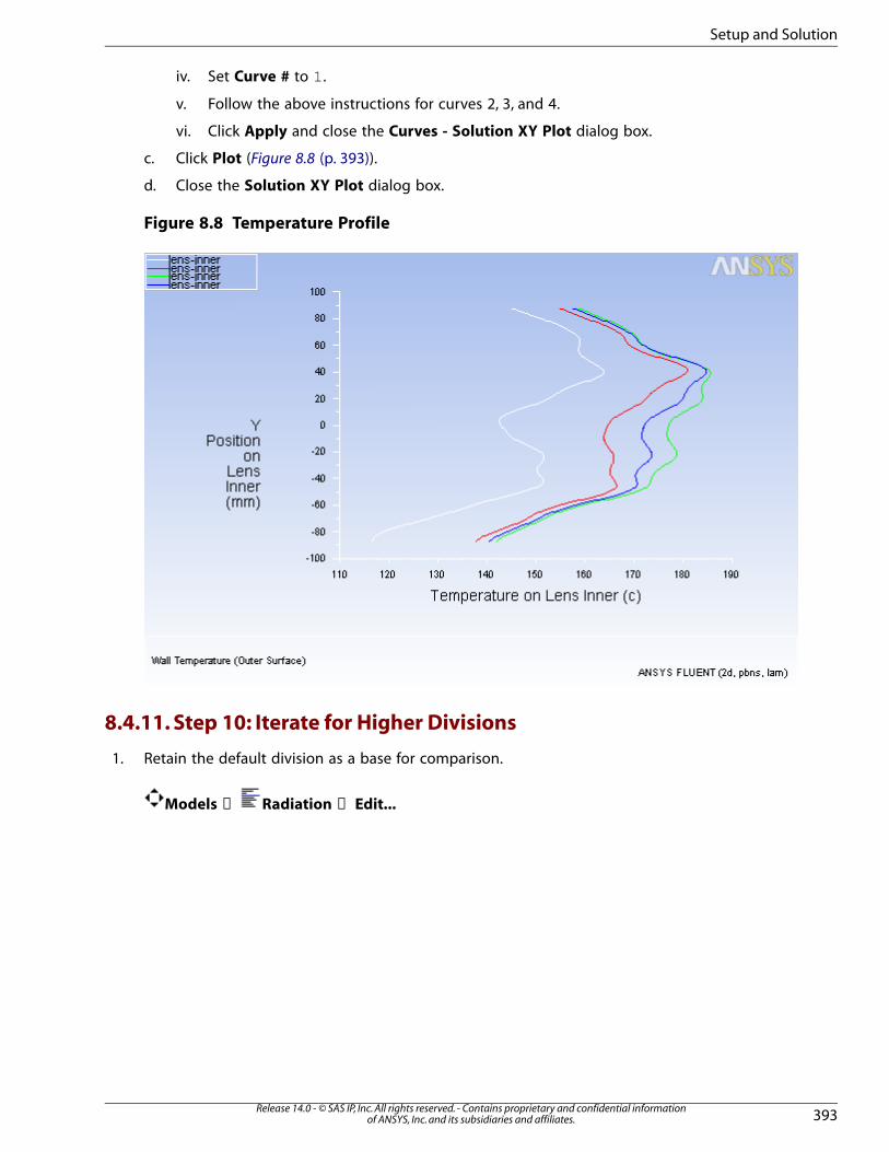
c. Click Plot (Figure 8.8 (p. 393)).
d. Close the Solution XY Plot dialog box.
Figure 8.8 Temperature Profile
8.4.11. Step 10: Iterate for Higher Divisions
1. Retain the default division as a base for comparison.
Models → Radiation → Edit...
393Release 14.0 - © SAS IP, Inc. All rights reserved. - Contains proprietary and confidential information
of ANSYS, Inc. and its subsidiaries and affiliates.
Setup and Solution
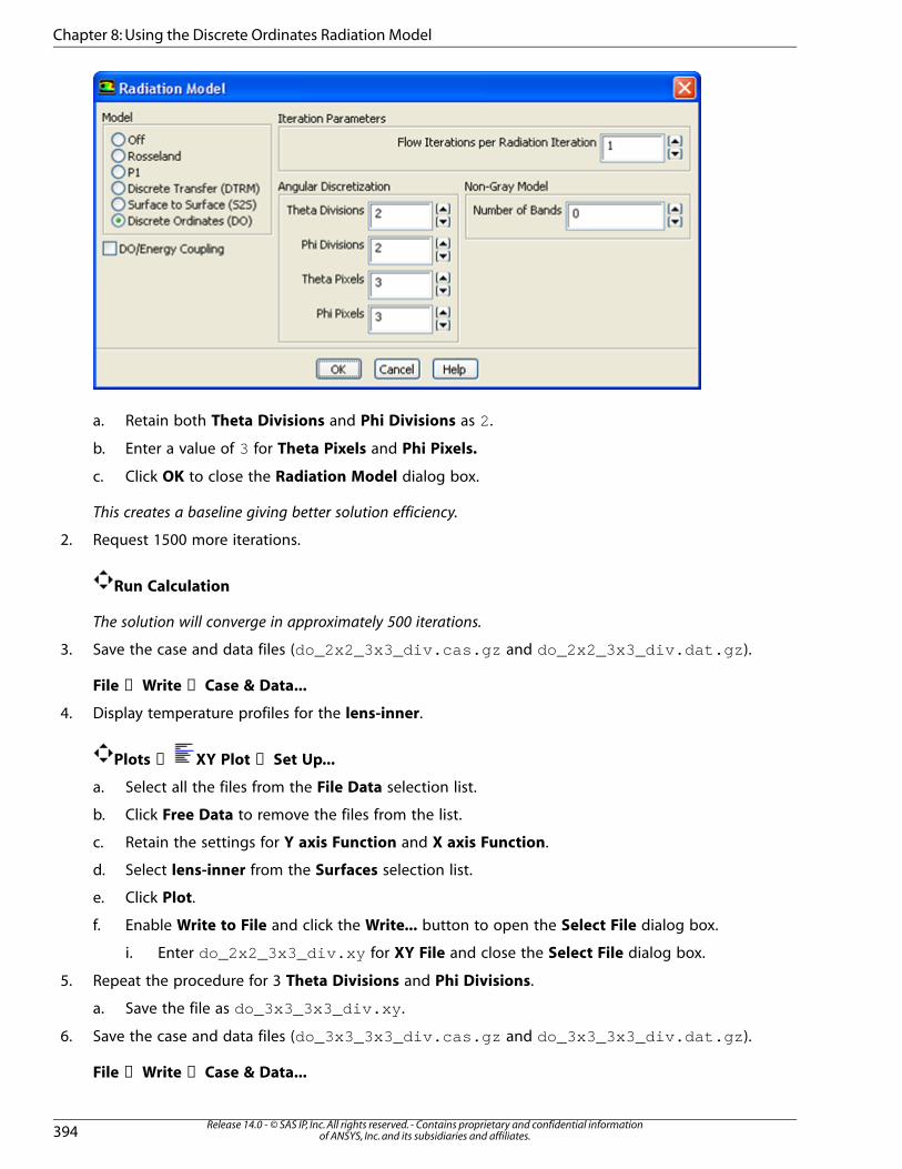
a. Retain both Theta Divisions and Phi Divisions as 2.
b. Enter a value of 3 for Theta Pixels and Phi Pixels.
c. Click OK to close the Radiation Model dialog box.
This creates a baseline giving better solution efficiency.
2. Request 1500 more iterations.
Run Calculation
The solution will converge in approximately 500 iterations.
3. Save the case and data files (do_2x2_3x3_div.cas.gz and do_2x2_3x3_div.dat.gz ).
File → Write → Case & Data...
4. Display temperature profiles for the lens-inner.
Plots → XY Plot → Set Up...
a. Select all the files from the File Data selection list.
b. Click Free Data to remove the files from the list.
c. Retain the settings for Y axis Function and X axis Function.
d. Select lens-inner from the Surfaces selection list.
e. Click Plot.
f. Enable Write to File and click the Write... button to open the Select File dialog box.
i. Enter do_2x2_3x3_div.xy for XY File and close the Select File dialog box.
5. Repeat the procedure for 3 Theta Divisions and Phi Divisions.
a. Save the file as do_3x3_3x3_div.xy .
6. Save the case and data files (do_3x3_3x3_div.cas.gz and do_3x3_3x3_div.dat.gz ).
File → Write → Case & Data...
Release 14.0 - © SAS IP, Inc. All rights reserved. - Contains proprietary and confidential informationof ANSYS, Inc. and its subsidiaries and affiliates.394
Chapter 8: Using the Discrete Ordinates Radiation Model

7. Repeat the procedure for 5 Theta Divisions and Phi Divisions.
a. Save the file as do_5x5_3x3_div.xy .
8. Read in all the files for Theta Divisions and Phi Divisions of 2, 3, and 5 and display temperature
profiles.
Make sure you deselect lens-inner from the Surfaces list so that no plots are duplicated.
Figure 8.9 Temperature Profiles for Various Theta Divisions
9. Save the case and data files (do_5x5_3x3_div.cas.gz and do_5x5_3x3_div.dat.gz ).
File → Write → Case & Data...
10. Compute the total heat transfer rate.
Reports → Fluxes → Set Up...
395Release 14.0 - © SAS IP, Inc. All rights reserved. - Contains proprietary and confidential information
of ANSYS, Inc. and its subsidiaries and affiliates.
Setup and Solution

a. Select Total Heat Transfer Rate in the Options group box.
b. Select all zones from the Boundaries selection list.
c. Click Compute.
Note
The net heat load is -0.025W, which equates to an imbalance of approximately 0.004%
when compared against the heat load of the bulb.
11. Compute the radiation heat transfer rate.
Reports → Fluxes → Set Up...
Release 14.0 - © SAS IP, Inc. All rights reserved. - Contains proprietary and confidential informationof ANSYS, Inc. and its subsidiaries and affiliates.396
Chapter 8: Using the Discrete Ordinates Radiation Model
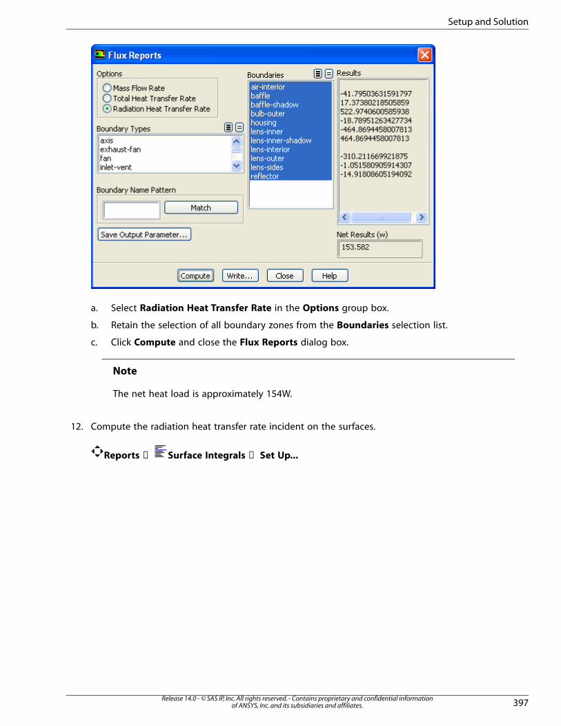
a. Select Radiation Heat Transfer Rate in the Options group box.
b. Retain the selection of all boundary zones from the Boundaries selection list.
c. Click Compute and close the Flux Reports dialog box.
Note
The net heat load is approximately 154W.
12. Compute the radiation heat transfer rate incident on the surfaces.
Reports → Surface Integrals → Set Up...
397Release 14.0 - © SAS IP, Inc. All rights reserved. - Contains proprietary and confidential information
of ANSYS, Inc. and its subsidiaries and affiliates.
Setup and Solution

a. Select Integral from the Report Type drop-down list.
b. Select Wall Fluxes... and Surface Incident Radiation from the Field Variable drop-down lists.
c. Select all surfaces except air-interior and lens-interior from the Surfaces selection list.
d. Click Compute.
13. Compute the reflected radiation flux.
Reports → Surface Integrals → Set Up...
Release 14.0 - © SAS IP, Inc. All rights reserved. - Contains proprietary and confidential informationof ANSYS, Inc. and its subsidiaries and affiliates.398
Chapter 8: Using the Discrete Ordinates Radiation Model

a. Retain the selection of Integral from the Report Type drop-down list.
b. Select Wall Fluxes... and Reflected Radiation Flux from the Field Variable drop-down lists.
c. Select all surfaces except air-interior and lens-interior from the Surfaces selection list.
d. Click Compute.
Reflected radiation flux values are printed in the console for all the zones. The zone baffle is facing
the filament and its shadow (baffle-shadow) is facing the lens. There is much more reflection on the
filament side than on the lens side, as expected.
lens-inner is facing the fluid and lens-inner-shadow is facing the lens. Due to different refractive in-
dexes and non-zero absorption coefficient on the lens, there is some reflection at the interface. Reflection
on lens-inner-shadow is the reflected energy of the incident radiation from the lens side. Reflection
on lens-inner is the reflected energy of the incident radiation from the fluid side.
14. Compute the transmitted radiation flux.
Reports → Surface Integrals → Set Up...
399Release 14.0 - © SAS IP, Inc. All rights reserved. - Contains proprietary and confidential information
of ANSYS, Inc. and its subsidiaries and affiliates.
Setup and Solution
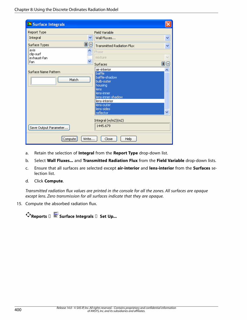
a. Retain the selection of Integral from the Report Type drop-down list.
b. Select Wall Fluxes... and Transmitted Radiation Flux from the Field Variable drop-down lists.
c. Ensure that all surfaces are selected except air-interior and lens-interior from the Surfaces se-
lection list.
d. Click Compute.
Transmitted radiation flux values are printed in the console for all the zones. All surfaces are opaque
except lens. Zero transmission for all surfaces indicate that they are opaque.
15. Compute the absorbed radiation flux.
Reports → Surface Integrals → Set Up...
Release 14.0 - © SAS IP, Inc. All rights reserved. - Contains proprietary and confidential informationof ANSYS, Inc. and its subsidiaries and affiliates.400
Chapter 8: Using the Discrete Ordinates Radiation Model

a. Retain the selection of Integral from the Report Type drop-down list.
b. Select Wall Fluxes... and Absorbed Radiation Flux from the Field Variable drop-down lists.
c. Ensure that all surfaces are selected except air-interior and lens-interior from the Surfaces se-
lection list.
d. Click Compute.
e. Close the Surface Integrals dialog box.
Absorption will only occur on opaque surface with a non-zero internal emissivity adjacent to particip-
ating cell zones. Note that absorption will not occur on a semi-transparent wall (irrespective of the
setting for internal emissivity). In semi-transparent media, absorption and emission will only occur as
a volumetric effect in the participating media with non-zero absorption coefficients.
8.4.12. Step 11: Make the Reflector Completely Diffuse
1. Read in the case and data files (do_3x3_3x3_div.cas.gz and do_3x3_3x3_div.dat.gz ).
2. Increase the diffuse fraction for reflector.
Boundary Conditions → reflector → Edit...
401Release 14.0 - © SAS IP, Inc. All rights reserved. - Contains proprietary and confidential information
of ANSYS, Inc. and its subsidiaries and affiliates.
Setup and Solution

a. Click the Radiation tab and enter 1 for Diffuse Fraction.
b. Click OK to close the Wall dialog box.
3. Request another 1500 iterations.
Run Calculation
The solution will converge in approximately 700 additional iterations.
4. Plot the temperature profiles after increasing the diffuse fraction for the reflector.
Plots → XY Plot → Set Up...
a. Save the file as do_3x3_3x3_div_df=1.xy .
b. Save the case and data files as do_3x3_3x3_div_df1.cas.gz and
do_3x3_3x3_div_df1.dat.gz .
Release 14.0 - © SAS IP, Inc. All rights reserved. - Contains proprietary and confidential informationof ANSYS, Inc. and its subsidiaries and affiliates.402
Chapter 8: Using the Discrete Ordinates Radiation Model
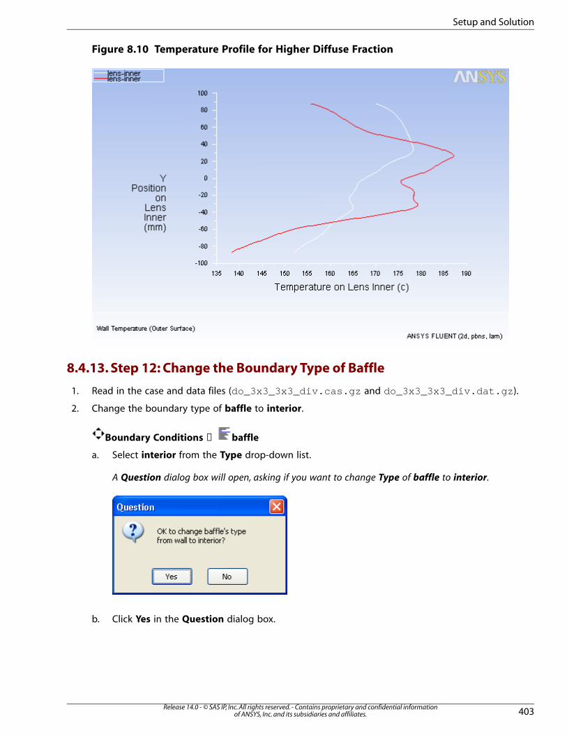
Figure 8.10 Temperature Profile for Higher Diffuse Fraction
8.4.13. Step 12: Change the Boundary Type of Baffle
1. Read in the case and data files (do_3x3_3x3_div.cas.gz and do_3x3_3x3_div.dat.gz ).
2. Change the boundary type of baffle to interior.
Boundary Conditions → baffle
a. Select interior from the Type drop-down list.
A Question dialog box will open, asking if you want to change Type of baffle to interior.
b. Click Yes in the Question dialog box.
403Release 14.0 - © SAS IP, Inc. All rights reserved. - Contains proprietary and confidential information
of ANSYS, Inc. and its subsidiaries and affiliates.
Setup and Solution

c. Click OK in the Interior dialog box.
3. Reduce the under-relaxation factors.
Solution Controls
a. Enter 0.5 for Pressure.
b. Enter 0.3 for Momentum.
4. Request another 2000 iterations.
Run Calculation
The solution will converge in approximately 1700 additional iterations.
5. Plot the temperature profile for baffle interior.
Plots → XY Plot → Set Up...
a. Save the file as do_3x3_3x3_div_baf_int.xy .
b. Save the case and data files as do_3x3_3x3_div_int.cas.gz and
do_3x3_3x3_div_int.dat.gz .
Release 14.0 - © SAS IP, Inc. All rights reserved. - Contains proprietary and confidential informationof ANSYS, Inc. and its subsidiaries and affiliates.404
Chapter 8: Using the Discrete Ordinates Radiation Model

Figure 8.11 Temperature Profile of baffle interior
8.5. Summary
This tutorial demonstrated the modeling of radiation using the discrete ordinates (DO) radiation model
in ANSYS FLUENT. In this tutorial, you learned the use of angular discretization and pixelation available
in the discrete ordinates radiation model and solved for different values of Pixels and Divisions. You
studied the change in behavior for higher absorption coefficient. Changes in internal emissivity, refractive
index, and diffuse fraction are illustrated with the temperature profile plots.
8.6. Further Improvements
This tutorial guides you through the steps to reach an initial solution. You may be able to obtain a more
accurate solution by using an appropriate higher-order discretization scheme and by adapting the mesh.
Mesh adaption can also ensure that the solution is independent of the mesh. These steps are demon-
strated in Introduction to Using ANSYS FLUENT: Fluid Flow and Heat Transfer in a Mixing Elbow (p. 131).
405Release 14.0 - © SAS IP, Inc. All rights reserved. - Contains proprietary and confidential information
of ANSYS, Inc. and its subsidiaries and affiliates.
Further Improvements

Release 14.0 - © SAS IP, Inc. All rights reserved. - Contains proprietary and confidential informationof ANSYS, Inc. and its subsidiaries and affiliates.406