chapter 8 the role of dbms in the new generation gis ... · pdf filechapter 8 the role of dbms...

Chapter 8

The role of DBMS in the new generation GIS architecture Sisi Zlatanova and Jantien Stoter

8.1 Introduction

Since the early ‘90, Geographical Information System (GIS) has become a

sophisticated system for maintaining and analysing spatial and thematic information

on spatial objects. DBMSs are increasingly important in GIS, since DBMSs are

traditionally used to handle large volumes of data and to ensure the logical consistency

and integrity of data, which also have become major requirements in GIS. Today

spatial data is mostly part of a complete work and information process. In many

organisations there is a need to implement GIS functionality as part of a central

Database Management System (DBMS), at least at the conceptual level, in which

spatial data and alphanumerical data are maintained in one integrated environment.

Consequently DBMS occupies a central place in the new generation GIS architecture.

An extended description on how GIS architecture has evolved can be found in

Vijlbrief and Oosterom van 1992. GISs used to be organised in a dual architecture

consisting of separated data management for administrative data in a Relational

DBMS and spatial data in a GIS. This was caused by different nature of

alphanumerical and spatial data, and the inability of early DBMSs to handle spatial

attributes. In the dual architecture (Figure 8.1 left) the two parts are connected with

each other via links based on unique id’s. The spatial attributes are not stored in the

DBMS and therefore they are unable to use the traditional database services such as

querying and indexing. In the dual architecture consistency of the data is hard to

manage. For example if a parcel is deleted in the spatial part, subjects can no longer

have a relationship with this parcel, which is maintained in the non-spatial part.

The solution to the problems of dual architecture was a layered architecture in

which all data is maintained in a single RDBMS. Since spatial data types were at that

time not supported at DBMS level, knowledge about spatial data types was maintained

in middle ware (Figure 8.1 middle). Spatial information was maintained in the DBMS

by means of Binary Large Objects (BLOBs). SQL cannot process data stored as

156

architecture, right: integrated architecture (courtesy of Vijlbrief and Oosterom van

1992).

Figure 8.1. Evolving architectures of GIS. Left: dual architecture; middle: layered

BLOBs and therefore the data depends on the host application code, which handles the

data in BLOB format. This solution requires data transport from the DBMS to middle

ware and consequently queries cannot be optimally implemented.

In recent times DBMSs are evolving towards an integrated architecture in which

all data is maintained in one object-relational DBMS (Figure 8.1 right). Presently,

most mainstream DBMSs support spatial data types and spatial functions by means of

Abstract Data Types (ADTs). This architecture is more beneficial for the integrity and

consistency of the data.

This chapter is devoted to the role of DBMS in new generation GIS architecture

and focuses on the manner spatial data can be managed, i.e., stored and analysed, in

DBMSs. Two important aspects of DBMS functionality are addressed in detail, i.e.,

spatial models and spatial analysis. Special attention is placed on the third

dimension (3D) because of the increased demand for 3D modelling, analysis and

presentations in many applications. The discussion in this chapter is restricted only

to vector models, i.e., raster models are outside the scope of this chapter.

The chapter is organised as follows: Section 8.2 outlines modelling of spatial

features in DBMSs, both using geometrical primitives and topological structure.

Section 8.3 makes an overview of possibilities to perform spatial analysis in DBMS.

Section 8.4 provides case studies and elaborated discussion on topology versus

geometry in DBMS. Section 8.5 is devoted to the third dimension. It starts with

examples of 3D GIS applications and elaborates on available techniques and new

developments required for full 3D support. The chapter ends with a discussion on

the role of DBMSs in the new generation GIS architecture considering both data

storage and spatial functionality.

Frontiers of Geographic Information Technology

157

multipolygon. The multipolygon is one type consisting of several polygons.

8.2 Spatial models in DBMS

A lot of progress is observed in the management of spatial and non-spatial information

for objects in one integrated DBMS environment, called a geo-DBMS. The

OpenGeospatial Consortium (OGC) largely contributed to this progress. The

OpenGeospatial Consortium adopted the ISO 19107 international standard (ISO 2001)

as Topic 1 of the Abstract Specifications: Feature Geometry99. These Abstract

Specifications provide conceptual schemas for describing the spatial characteristics of

spatial objects (geographic features, in OGC terms) and a set of spatial operations

consistent with these schemas and with vector geometry and topology up to three

dimensions embedded in 3D space. According to the specifications, the spatial object

is represented by two structures, i.e., geometrical structure, i.e., simple feature, and

topological structure, i.e., complex feature. While the geometrical structure provides

direct access to the coordinates of individual objects, the topological structure

encapsulates information about their spatial relationships.

The OGC Abstract Specifications have been transformed into Implementation

Specifications, of which the most relevant for DBMSs is the OGC Simple Features

Specification for SQL (OGC 1999), which provide guidance on how spatial objects

have to be maintained in object relational DBMS environments. Sub-section 8.2.3

briefly describes the implementation strategies of mainstream DBMSs. Since the

native maintenance of topology by DBMS is still in an ascent stage, special attention

is paid to topological models. The problems associated with 3D topological models as

well as some prototype implementations are discussed in detail.

8.2.1 Geometrical primitives in DBMS

Informix (Informix 2000), Ingres (Ingres 1994), Postgres (PostGIS) and MySQL have

implemented spatial data types and spatial operators more or less according to the

Simple Features Specification for SQL of OGC. The implementation is based on

Abstract Data Types (ADTs) that support storage, retrieval, query and update of

simple spatial features, i.e., points, lines and polygons, and a set of spatial operations

built on top of them.

Currently, no 3D primitive is implemented. However, most DBMSs, including

Oracle, Postgres, IBM, Ingres, Informix, support the storage of simple features in

3D space. In general, it is possible to store for example a polygon in 3D. 3D

volumetric objects can be stored in a geometrical model as polyhedrons using 3D

polygons, i.e., a body with flat faces, in two ways: as a set of polygons or as

The role of DBMS in the new generation GIS architecture

To date, mainstream DBMSs such as Oracle, (Oracle 2001), IBM DB2 (IBM 2000),

158

Our tests with different representations have shown advantages and disadvantages of

both approaches (Stoter and Zlatanova 2003). An advantage of 3D multipolygons

compared to list of polygons is that they are identifiable as one object by front-end

applications, e.g., GIS and CAD, which can access objects stored in the DBMS.

Furthermore, this approach has one-to-one correspondence between a record and an

object. The major disadvantage of both implementations is that the DBMS does not

recognise the 3D object, e.g., volume cannot be computed. In addition, spatial

functions on 0D, 1D and 2D primitives defined in 3D space project the spatial data on

a 2D plane. The way out is support of real 3D volumetric data types. A possibility of

this work, a 3D primitive as polyhedron is defined as part of the geometrical spatial

model of Oracle Spatial, including validation functions and spatial functions in 3D.

8.2.2 Topological structures in DBMS

Topological structures are generally used to represent planar or space partitions

without redundancy and to represent (linear) networks. In planar and space partitions,

spatial objects are defined on the basis of non-overlapping partitions. A large number

of 2D topological structures are already available in the literature, of which some of

them have been implemented in commercial and non-commercial systems and

populated with data (LaserScan100; Oosterom and Lemmen 2001; Oracle Spatial

10g101). Many 3D topological structures are also reported but only a few of them are

further extended to support spatial operations.

OGC has also recognised the need for topology standardisation. Implementation

Specifications for topological structures, i.e., complex features in OGC terms are

currently being developed by the OpenGeospatial Consortium in cooperation with

ISO. The new interfaces will build on the OGC Simple Features Specification to

address feature collections and more complex objects and concepts including curves

and surfaces in 2D and 3D, compound geometries, arcs and circle interpolations,

conics, polynomial splines, topology and solids. The interfaces will cover creation,

querying, modifying, translating, accessing, fusing, and transferring spatial

information.

To illustrate current state of the art of topological structure in DBMS, this section

continues with the view of OGC and ISO about topological primitives (sub-section

8.2.2.1), a non-commercial implementation of 2D topological structure (sub-

section 8.2.2.2) and commercial solution LaserScan Radius Topology100 and Oracle

Spatial 10g (sub-section 2.2.3). Similarly to a 3D geometrical primitive, 3D

topological structure has not (yet) been implemented as part of a DBMS. Sub-section

2.2.4 describes non-commercial implementations of a 3D topological structure.

having a 3D geometrical primitive at DBMS level is shown in Arens et al. 2003. In


159

8.2.2.1 ISO and OGC about primitives

‘Face’ is the topological equivalent of the geometrical primitive ‘polygon’. There is a

slight difference between the definitions of face and polygon in ISO and the OGC

specifications for SQL.

According to the ISO standard a face is defined by edges as the orientation is

strictly defined (anti-clockwise). A face can have holes (called inner rings) and the

orientation of the edges is in clockwise order. Every edge has a reference to preceding

and succeeding edges. The definition of a polygon needs refinements. For example, it

is not clear whether the outer boundary of a polygon is allowed to touch itself nor is it

2003). However, since only one outer boundary is allowed, a polygon with two outer

boundaries defining potentially disconnected areas is certainly invalid.

As was stated before, the OpenGeospatial Consortium adopted the ISO Spatial

Schema as Abstract Specifications and transformed these to the implementation level

in the OGC Simple Feature Specification for SQL. Since the OGC Specifications for

SQL are based on geometry, only the geometrical primitives are defined. A polygon is

defined as a simple, planar surface. Rings may touch each other in at most a point and

self-intersection of outer and inner rings is not allowed (Oosterom et al. 2003). Inner

rings, which divide the polygon in disconnected parts, are also not allowed. Note that

OGC does not address orientation of polygons.

8.2.2.2 Non-commercial implementation of 2D topological structure in DBMS

A lot of implementations of non-commercial 2D topological models are currently in

use. An excellent example is the topological model developed and implemented by the

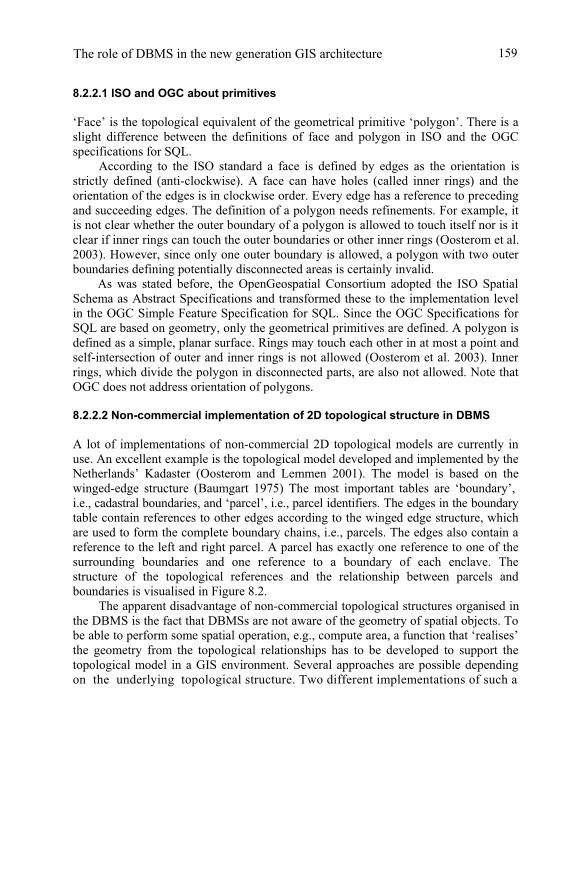
Netherlands’ Kadaster (Oosterom and Lemmen 2001). The model is based on the

winged-edge structure (Baumgart 1975) The most important tables are ‘boundary’,

i.e., cadastral boundaries, and ‘parcel’, i.e., parcel identifiers. The edges in the boundary

table contain references to other edges according to the winged edge structure, which

are used to form the complete boundary chains, i.e., parcels. The edges also contain a

reference to the left and right parcel. A parcel has exactly one reference to one of the

surrounding boundaries and one reference to a boundary of each enclave. The

structure of the topological references and the relationship between parcels and

boundaries is visualised in Figure 8.2.

The apparent disadvantage of non-commercial topological structures organised in

the DBMS is the fact that DBMSs are not aware of the geometry of spatial objects. To

be able to perform some spatial operation, e.g., compute area, a function that ‘realises’

the geometry from the topological relationships has to be developed to support the

topological model in a GIS environment. Several approaches are possible depending

on the underlying topological structure. Two different implementations of such a


clear if inner rings can touch the outer boundaries or other inner rings (Oosterom et al.

160

(courtesy of Oosterom and Lemmen 2001)

Figure 8.2. Topological structure in the spatial DBMS of the Netherlands’ Kadaster

uses the information on the relationship between edges. The second solution is based

on the left-right information of edges. In the first implementation, the function creates a polygon geometry according

Oracle Spatial and ISO rules: the coordinates of the outer ring are listed in anti-

clockwise order and the coordinates of the enclaves are listed in clockwise order. To

generate the parcel polygon, the function starts with the first boundary, which is

referred to in the parcel table. Then the connecting boundary in anti-clockwise order is

found. This step is repeated until the polygon is closed. The polygon is constructed by

connecting all linestrings of the found boundaries. In case of enclaves, the same

procedure is followed but in clockwise order.

The second implementation of the ‘return_polygon’ function uses only the left-

right information stored with every parcel boundary and a (geometrical) comparison to

find and join connected boundaries in a ring. Here the boundaries that have the given

parcel to the left or to the right are selected. The boundary of the parcel is composed

by repeatedly joining boundaries that end at the same endpoint. Enclaves are realised

in the same way. The orientation of the rings, i.e., clockwise or counter-clockwise does

not follow from the algorithm and must be calculated afterwards.

The implementations differ in the underlying geometrical primitive. In the

winged-edge implementation the outer ring of a face can touch itself in the outer

boundary at exactly one point and in the left-right implementation this is not possible.

This difference can be illustrated by the polygon as shown in Figure 8.3: a polygon

function called ‘return_polygon’ are presented by Quak et al. 2003. The first solution


161

that has an island that touches the boundary in exactly one point. The relationship-

between-edges algorithm will generate a polygon with one self-touching outer ring

which is not valid according to the OGC definition, while the left-right algorithm will

return a polygon with a boundary and an island.

8.3. A polygon with a hole that touches the boundary

The performance of both implementations also differs and is dependent on the

complexity of the data: the more points in a boundary, the worse the performance.

This is especially true for the left-right implementation, where the computational cost

increases with the number of points. Also the more boundaries there are in a polygon,

the worse the performance. This is especially true for the relationship-between-edges

implementation since the more boundaries there are; the more select statements need

to be performed.

8.2.2.3 Commercial implementation of 2D topological structure in DBMS

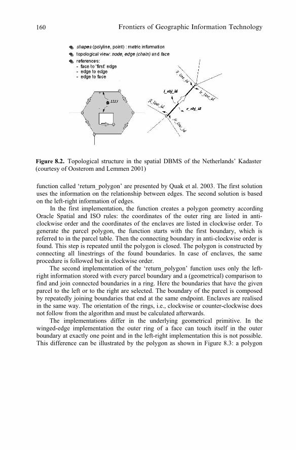
Compared to the user-implemented models, the implementation of topology structure

in LaserScan Radius Topology100 is much more extensive, it is a ‘complete’

implementation of topology with support for linear networks and planar topology,

including updates, insertions and deletions. All required topological references are

stored explicitly: the winged edge representation in the edge-to-edge table makes up

just a small part of the complete system (see Figure 8.4). Topological primitives are

stored in the NODE, EDGE and FACE tables while faces are only stored by references

to edges. A number of reference tables are used to store various types of topological

references. The TOPO table is the link between the features and the topological

structures. Topology is organised in ‘manifolds’. Associated with each manifold and

with the system as a whole are some metadata and error tables. Before topologically

structuring data in Radius Topology, the user can specify rules in order to control the

way the structuring works, such as snap tolerances, which features/primitives are

moved and which stay while snapping, etc.

To realise geometry from a topologically structured dataset Radius offers a

‘get_geom’ function that is equivalent to the ‘return_polygon’ function of the non-

Figure


162

8.4. Radius Topology database tables (version 1.0), taken from LaserScan100 Figure

commercial implementations as described above. Most users however choose not to

use this function, but instead store a copy of the geometry explicitly. This increases the

storage requirements, but it means that there is no performance penalty when

accessing geometries (e.g., for display or geometric queries) since the geometry is

instantly available and does not have to be computed. The use of database triggers in

the Radius Topology architecture ensures that the geometries and their topological

representation are always synchronised. Additionally support for topological querying

(containment, adjacency, connectivity, overlap) is available by means of a topo_relate

operator.

Louwesma et al. (2003) describe a performance test in which topology structure

of Laserscan Radius Topology was compared to the geometrical primitive of Oracle

Spatial 9i. In the topology case less points are stored by avoiding storing ‘common’

boundaries twice. However disk space requirements where much bigger in the

topology case due to the increased number of topology primitives and references

between them compared to the number of area features and the way geometry is


163

implemented in Oracle Spatial, small objects have relatively much overhead. The total

storage requirement for topology is intended for references, id’s and associated

indexes that are required for the Radius topology structure. The storage requirement

will probably be more favourable towards topology in the case of smaller scale data

and data with a relatively high number of intermediate points in the boundaries.

From the tests described in (Louwesma et al. 2003) it can be concluded that

performance of geometrical querying on a data set topologically structured with

Radius Topology is slower. This is due to the cost of computing the geometries on-

the-fly from the topological information. This occurs when geometries are not stored

explicitly alongside the topology. For this reason users often store the geometries

explicitly as described above.

Oracle Spatial 10g also supports 2D topology101. The basic topology elements in

an Oracle topology are nodes, edges and faces. A node is represented by a point and

can be used to model an isolated point feature or edges. Every node has a coordinate

pair associated with it to describe the spatial location of the node. An edge is bounded

by a start- and an end-node and has a coordinate string describing the spatial

representation. Each edge can consist of multiple vertices, represented by linear as

well as circular arc strings. As each edge is directed, it is possible to determine which

faces are located at the left and right hand side of the edge. A face is represented by a

polygon (that can be reconstructed from the several edge strings) and has references to

a directed edge on its outer and (if any) inner boundaries. Each topology has a

universal face that contains all other nodes, edges and faces in the topology.

Penninga and colleagues (Penninga 2004) tested the support of topology with two

data sets from the Netherlands cadastre. The tests have shown that the current

implementation does not completely avoid redundant data storage. The geometry is

stored both in node and edge tables. However, as long as the user uses the supplied

tools for data editing instead of directly updating the node, edge and face tables, data

consistency can be efficiently maintained. In general Oracle topology can be

considered a very suitable solution for the average user. The expert user might need to

edit directly on the node, edge and face tables, as it is much quicker. More

experiments are needed to explore the offered functionality.

8.2.2.4 Non-commercial 3D topological structures in DBMS

In 3D, there is no consensus on a single topological structure. Different topological

structures can be defined depending on the number of primitives to maintain, and also

the number and nature of relationships to explicitly store. The problems of defining 3D

topological structures are relatively many compared to 2D. Due to the large amounts

of data and higher complexity, one data structure representing a specific topological

structure, which is appropriate for a certain application, may not be easy to serve

another application. Unfortunately, 2D topological structures are not directly

extendable to 3D. 2D structures are mostly built around the properties of an edge. One


164

8.5. UML class diagram of Simplified Spatial Model (Zlatanova 2000).

Figure

edge has exactly two neighbouring nodes (begin and end) and exactly two

neighbouring faces (left and right). This property is not true in 3D space. An edge can

have more than two neighbouring faces, i.e., the order of the faces has to be specified.

An extensive study on 3D topological structures is presented in Zlatanova et al. (2004).

One of these 3D structures (i.e., the Simplified Spatial Model, Zlatanova 2000) has

been used to test 3D topological implementations in object-relational DBMS. In this

structure, edges are not explicitly stored due to performance considerations (Coors

2003). The role of the edge (=boundary) in 2D is now overtaken by the face

(=boundary). Nodes describe faces and faces describe bodies. The 1D primitive as part

of a body, is not explicitly stored (see Figure 8.5).

This 3D topological structure can be implemented in various ways in a relational

DBMS. The first straightforward approach is the relational implementation. The

conceptual model can be converted directly into a relational data model. For each

object (node, face, and body) a separate relational table is created. The NODE table

contains the identifier of the node and the three coordinates. The FACE table contains

the id of the face, a column denoting the anti clockwise order of the nodes in a face

and the id’s of nodes that the face consists of. A BODY table contains references to

the id’s of faces it consists of. Since the relationship between a face and constituting

nodes is one-to-many (1:m), multiple rows represent one face. Theoretically, it is

possible to have a separate column for each node but this approach is beneficial only

in case the faces are triangles. Such an approach is reported by Coors (2003).

Another possibility is the object-relational implementation. The list of id’s

referring to lower-dimensional objects (faces, nodes) is stored in a newly defined

object of type ‘variable array’ or ‘nested table’. Such a new object type can

consequently be stored in a single column. This means that the number of rows in the

object table is reduced to the actual number of the higher dimensional object (body,

face). Object relational implementation is a two-step procedure, i.e., creating objects

(ADTs) and creating tables with columns of the created data types. Similarly to the 2D case, the major disadvantage is that the DBMS is not aware of

the spatial object. Spatial operations and spatial indexing offered by spatial DBMS

cannot be used. To be able to use the spatial operations of DBMS, a function similar to


165

‘return-polygon’, as mentioned above for the 2D case, has been defined (Zlatanova

2001). This function realises the geometry of the 3D spatial objects, based on the

topological tables and returns a 3D geometrical primitive as described before, i.e., a

polyhedron consisting of flat polygons defined in 3D.

In general, regardless the type of topological structure used, the implementations

have similar disadvantages as the ones specified for 2D user-implemented topological

structures, i.e., the performance is relatively slow for certain queries. Operations on the

topological model have to be further developed, to be able to use DBMS spatial

operations, realisation has to be first performed. However, simple SQL statements

comparing the identifiers of constituent primitives can perform a large number of

topological operations. Section 8.3.3 describes a case study that illustrates the power

of topological models in spatial analysis.

8.3 Spatial analysis in DBMSs

Spatial functionality is related to operations that are performed on spatial objects as

very often no distinction is made between spatial and thematic components. In this

chapter we will concentrate on the part of spatial functionality that is related to the

spatial component. The most important aspect in the spatial domain is the framework

for detecting spatial relationships. Amongst the different approaches (topology,

distance, order, etc.) GIS society has largely accepted topology. OGC has adopted

three topological frameworks: Boolean set of operations, Egenhofer operators and

Clementini operators. Using these frameworks a large number of operators can be

developed. However, the question ‘who is responsible for the implementations’ (front-

end applications or spatial DBMS) is still open and even extensively discussed.

Although several studies have shown that it is better to perform spatial operations

close to the data, GIS vendors might not be willing to give up spatial analyses. In

addition since spatial analyses in GISs have a long history, at least in the short-term

feature spatial analyses in GIS front-ends will show better performance.

In the introduction (section 1) the new generation GIS architecture was made

clear, in which all spatial data is maintained (and recognised as such) at DBMS level,

without the intervention of middle-ware software. The functionality concerning spatial

analyses that DBMS has to offer in such an architecture depends very much on the

scope and constraints of spatial analysis: what is spatial analysis and what is spatial

analysis in the DBMS context. DBMSs are essential in applications in which large

amounts of large-scale geo-data need to be maintained and managed, such as cadastral

data or spatial data used in municipalities. In general we can say that GIS

functionalities that are not specific to a certain application belong in the DBMS and

not in GIS (or CAD) front-ends. Examples are the spatial functions that examine the

topological relationships between spatial objects. Arguments for this are the logical


166

consistency of the data, better performance and better maintenance of the data, since

unnecessary transport and conversions of data between DBMSs and GIS front-ends

prone to errors can be avoided. On the other hand spatial functions that are specific

for certain applications should be implemented in front-ends.

Here we consider the spatial analyses at DBMS-level that should be present to

support the new generation GIS architecture. We will also give an overview on the

spatial analyses that are currently supported in DBMSs. In the discussion (section 8.6)

we will refine the statement on where spatial analyses should fit within the optimal

architecture based on (past) trends both in computing technology, as well as in GIS.

8.3.1 Which operations in DBMS?

DBMS has not been designed to manage spatial objects, but does have a strictly

defined functionality based on relational algebra and calculus (Ramakrishnan and

Gehrke 2003). In principle, three generic operations are distinguished in the database

literature (e.g., Tsichritzis and Lochovsky 1982): insert (add new data), delete (remove

data from the database) and update (change existing data). A similar set of generic

operations (but more elaborated) has to be available for spatial data. The operations

related to introducing a new element, deleting and updating an existing one have to be

extended with respect to the structure used, i.e., geometry or topology. Examples of

such operations can be:

• operations to organise the data according to the used topological structure, i.e.,

operations for planarity, convexity and discontinuity as they are defined in

the model.

• operators for consistency check: validation of the objects (e.g., polygon

closed, body closed), node-on-line, node-on-face, node-in-body, line-on-face,

line-in-body, intersection of lines, face-on-face, intersection of faces, face-in-

body.

In addition to generic operations, DBMS offers a set of more elaborated operations

known as selection, navigation and specialisation:

• selection: retrieve operation under a particular condition;

• navigation: describe the process of travelling through the database, following

explicit paths from one record to the next in the search for some required

piece of data;

• specialisation: complex operation that allows a new object to be created on

the basis of existing ones.


167

Also these three generic operations have to be available for spatial data in a spatial

context.

Selection in a spatial context is an operation that allows a number of data to be

identified on the basis of three properties, i.e., logical position (first, last, prior), value

of the content and/or relationship. An example of spatial selection operation is ‘select

all the buildings that are located next to the park’. Furthermore, three basic groups of

spatial selection operations should be offered at database level (Zlatanova et al. 2004):

• metric operations: selection operations, requiring computations of geometric

properties e.g., compute distance, volume, area, length, centre of gravity. The

metric operations need coordinates of the spatial objects and the result is

always quantitative.

• proximity operations: These are selection operations related to spatial

location, e.g., objects in a certain area/volume, field of view. Position

operations largely benefit of the spatial index offered by DBMS to restrict the

search.

• relationship (topology) operations: selection operations based on spatial

relationships. These operators will be dependent on the framework for

detecting relationships. If topology is considered, the abstract specifications

recommend three frameworks for implementation as was described before.

Depending on the implementations (framework and model), topology

operations are the ones expected to perform better on a topological model.

Besides selection, navigation and specialisation operations in a spatial context

have to be also considered at DBMS level. Navigation is an operation that permits a

logical path to be followed on the basis of a selection. Examples of spatial navigation

operations are route planning (e.g., multiple topology operations ‘meet’), shortest path

(multiple topology operation ‘meet’ and multiple metric operation ‘distance’) and

intervisibility. The navigation (in the database sense of the word, as it was explained

above) should not be equated with spatial navigation (in the shortest-path sense). The

latter is more of an analysis process using the data from the database and other

external algorithms not standard within SQL or the DBMS. However, spatial

navigation operations use the inbuilt navigation capabilities of the DBMS.

Examples of spatial specialisations are buffer, convex hull, union of objects and

all types of generalisations. While navigation might be based only on topological

operations, specialisations need in most of the cases the coordinates of objects.

However, additional information retrieved on the basis of proximity or topology

operations may be of use for some specialisations, e.g., union or generalisation.

In contrast to the group of selection operations, specialisation and especially

navigation in the spatial domain can be very complex and time consuming. If they are

performed at a DBMS level on the server, the performance can decrease drastically.


168

Furthermore, such complex operations may not be needed for all kind of applications.

Therefore, these operations could be considered for implementation by the front-end.

8.3.2 Spatial operations currently offered by DBMSs

The spatial functionality presently offered by mainstream DBMS covers in general

lines the scope of operations discussed in the previous sub-section. We use Oracle

Spatial 9i to illustrate the possibilities of spatial analysis in DBMSs.

At database level, spatial operations can be defined utilising either geometrical or

topological representations. It should be noticed (again) that the operations presently

offered by the mainstream DBMS vendors (an exception is Oracle Spatial 10g) are

built on the geometrical model due to lack of topology maintenance and therefore they

work directly on the geometry (no geometrical realisation is needed). Oracle Spatial 9i

supports the three groups of selection operations, i.e., topology operations, a variety of

metric operations, proximity operations as well as simple specialisation operations.

Another class of specialisation operations returns an aggregate of a collection of

geometries. These are not defined within OGC. Tables 8.1 and 8.2 show examples of

spatial functions implemented by Oracle Spatial and the equivalent OGC functions.

OGC Oracle

Equals EQUAL

Disjoint DISJOINT

Intersects ANYINTERACT

Touches TOUCH

Crosses OVERLAPBDYDISJOINT

Within INSIDE

Contains CONTAINS

Overlaps OVERLAPBDYINTERSECT

Table 8.1. Topological operations in the DBMS according to Implementation

Specifications of OGC and Oracle implementations

Unary operations OGC Oracle

Convexhull SDO CONVEXHULL

Area SDO AREA

Buffer SDO BUFFER

Centroid SDO CENTROID

Length SDO LENGTH

Boundary SDO MBR


169

Binary operations

OGC Oracle

Distance SDO DISTANCE

Intersection SDO INTERSECTION

Union SDO UNION

Difference SDO DIFFERENCE

Symdifference SDO XOR

Table 8.2. Metric and position operations according to Implementation Specifications

of OGC and Oracle implementations

Although not that common, spatial analysis on topological structure is also

available, e.g., Laser-Scan Radius Topology, Oracle Spatial 10g, but the knowledge is

still limited. One of the most important operations, i.e., the realisation of geometry was

already discussed in Section 8.2. The complexity of the functions considerably varies

with respect to the different implementations. For example, the geometry (coordinates)

of a body can be extracted by only one SQL statement in the case of relational

implementation if the geometry is maintained explicitly, but an embedded script is

required if the body is represented as ‘variable array’ of polygons.

In principle, all the topology operations have to perform better on the topological

model than on geometry alternatives. On the other hand, some operations (compute

area, distance, etc.) on topological structured data will be slower than on geometrical

primitives since it requires querying and joining different relational tables, which is

also discussed in (Hoel et al. 2003). Another explanation for the better performance of

these spatial operations on the geometrical model is the internal optimisations

provided by the DBMSs and the possibility to apply spatial indexes.

8.4 Topology or geometry

The statement that topological querying (queries that only require explicitly stored

relationships) is much faster than in the situation where only simple geometry is

available, was tested in a case study described in section 8.4.1. In section 8.4.2 it is

discussed what to prefer: topologically structured data or geometrically structured

data.


170

8.4.1 Case study

To illustrate the power of topological structure in performing relationship operations,

we did an experiment in Oracle Spatial 9i, on a dataset, which is a selection of the

cadastral database of the Netherlands. The test data set contains 1,788,019 parcels and

5,599,089 boundaries. The topological structure used for this dataset is described in

section 8.2.2.4.

The query that we use in this experiment is to find all adjacent parcels to the

parcel with object identifier 6862 (see Figure 8.6). The query was performed on both

a topologically structured dataset and a geometrically structured dataset. The

geometries of the parcels were therefore stored explicitly in the geometrical primitive

of Oracle Spatial by means of the return_polygon function (section 8.2.2.2). A spatial

index was built on the geometry-column to speed up spatial analyses.

For the data set described by geometrical primitives, the query to find all adjacent

parcels is given below using a ‘subselect’ structure, in which the polygons of parcels

are stored in the table ‘parcels_geom’ in the column named ‘shape’.

select object_id from parcels_geom where sdo_relate(shape, (select shape from parcels_geom where object_id=6862), ‘MASK=TOUCH’) = ‘TRUE’;

The query uses the built spatial index.

parcel 6862’.

Figure 8.6. Data set used to perform the test query: ‘find all parcels adjacent to


171

The query finds all parcels that have a ‘touch’ relationship with parcel ‘6862’

using the spatial operator ‘sdo_relate’ which is implemented on geometrical

primitives. The result is:

OBJECT_id ------------- 7142 2067 2066 7141 2065 6862 6861 7 rows selected. Elapsed: 00:00:22.05

In the topologically structured data set, all adjacent parcels to parcel ‘6862’ can be

found when all the boundaries are selected that have the specific parcel on the left or

right side. The next step is to find the parcel that is located on the other side of the

selected boundaries:

select l_obj_id, r_obj_id from boundary where r_obj_id=6862 or l_obj_id=6862;

The result is: L_OBJ_id R_OBJ_id -------------- ----------- ----- 2066 6862 6862 7141 6861 6862 6862 7142 Elapsed: 00:00:00.01

The same test was performed for parcel ‘7142’ with 28 adjacent parcels. The

processing time for this second query was 22.56 seconds for the geometrical query and

00.01 seconds for the topological query. The queries were repeated a number of times

which resulted in processing times of the same order every time. These examples show

that the topological query is indeed faster on a topologically structured data set than on

data set described with the geometrical primitives.

There is another conclusion that can be drawn from the first query: the results differ.

The topological query does not give parcels ‘2067’ and ‘2065’ as a result since these

parcels touch parcel ‘6862’ only at a point and are therefore not seen as adjacent parcels


172

from the topological point of view as defined in the winged-edge structure. The result set

in spatial analyses using topological structure is therefore dependent of the topological

structure implemented. The geometrical query does find parcels ‘2067’ (neighbour on

the right of parcel ‘2066’) and ‘2065’ as adjacent parcels since they do touch parcel

‘6862’, even if it is only at a point. The geometrical query could be further specified by

adding the condition that boundaries of two parcels should also overlap.

Although this case study is related to 2D data, a 3D comparison case study could

even show bigger differences, as geometrical queries in 3D require more complex

algorithms than 2D functions. This has a big influence on the computational

complexity of topological queries that work on 3D geometrical primitives compared to

topological queries that work on topologically structured data.

8.4.2 Discussion

The question whether or not to manage topology in DBMS is still challenging.

Extensive argumentation for the need to organise the topology at DBMS level is given

• it avoids redundant storage and is therefore more compact than a geometrical

model

• it is easier to maintain the consistency of data after editing

• it is more efficient during the visualisation in some types of front-ends,

because less data has to be read from disk and transferred to clients

• it is the natural data model for certain applications; e.g., during surveying an

edge is collected together with attributes belonging to a boundary

• it is more efficient for certain query operations, e.g., find neighbours

On the other hand geometrical queries on topological structure are much slower than

on geometrical primitives, since a geometrical realisation is always required, by which

several tables need to be queried that contain the lower dimensional objects. The same

is true for visualisation of spatial data. Another problem of topologically structured

data is the required storage capacity compared to the storage capacity needed for the

geometrical primitives. Every row in the tables defining the topological structure has

its overhead, and the references require a lot of storage capacity. An advantage of the

topological structure is that topology structure management can be used in storage

(maintaining consistency), data management and retrieval of data.

In principle, we believe that only one model, i.e., topological model, should be

sufficient to manage spatial data in DBMS. However since performance of

geometrical queries as well as of visualisation favours the geometrical model, which

will be even more apparent in 3D, it could be argued that a DBMS that support both

in Oosterom et al. 2002a. Some of the advantages are listed bellow:


173

models simultaneously would be the most appropriate solution. In this case spatial

objects are maintained in geometrical primitives and topological structure

simultaneously and triggers are defined between the two representations to keep the

two different representations up-to-date. Of course this solutions undermines the

argument that topology structure avoids redundancy of the data. Another disadvantage

is that the storage of spatial data becomes even less efficient compared to the

topologically structured data.

8.5 3D and Geo-DBMS

The need for 3D information is rapidly increasing. Many examples of applications that

have a growing interest in 3D information have been cited (Oosterom et al. 2002b;

Oosterom et al. 2002c). Traditionally, the military applications were the first to look

for 3D solutions and provided the first elaborated systems for 3D visualisation and

the third dimension. In this section first examples of the growing need for 3D geo-

information are given (section 8.5.1). In the second subsection (8.5.2) the question is

addressed whether current DBMS technology is appropriate to meet the growing need

for 3D geo-information.

8.5.1 Growing need for 3D information

The growing need for 3D geo-information is felt in different disciplines:

Applications in urban areas

• Urban planning is one of most demanding areas pushing 3D developers to

provided fast modelling approaches, extended visualisation, interaction tools,

influence of new buildings and infrastructure on the existing environment can

be best visualised in 3D environments using virtual reality or augmented

reality environments such as in Figure 8.7, which is important for

presentation to citizens. In addition, 3D visualisations of planned

infrastructure and underground constructions enables providing more insight

into the vertical planning of regions.

• Cadastres traditionally register property rights to real estate on 2D parcels

since the individualisation of land started with a subdivision of land using 2D

boundaries. In today’s world there is growing pressure on land that has led to

stratified property (property units on top of and engaging each other).

Cadastres throughout the world are confronted with the challenge how to


simulation (Lindstrom et al. 1996). Nowadays more and more civil applications need

and elaborated spatial functionality (Nebiker 2003; Shi et al. 2003). The

174

register and visualise stratified properties. This requires an extension of the

cadastral map in 3D (Figure 8.8) (Oosterom and Lemmen 2003).

• Pipelines and tunnels can be better protected against damage when their 3D

location can be visualised in the real world (Roberts et al. 2002). For

example, knowledge about the location of cables and pipelines can avoid

damage during excavation. Based on knowledge of the location of

constructions precisely defined restrictions can be imposed on the owners of

the surface land from doing anything that could damage the underground

construction.

• Location-based services (LBS) for shopping, tourism, rescue operations etc.

is another area, where the use of 3D visualisation and most probably 3D GIS

Applications in non-urban areas

• Road, railway, canal construction and maintenance benefits largely by 3D

environments (Bresters 2003).

• Landscape modelling seeks specific 3D tools for interactive design and

simulation (Lammeren et al.102; Blaschke and Tiede 2003).

• In telecommunications the decision on the locations of antennas requires 3D

analyses to obtain information on the area that can be covered and on the

costs of using the specific location.

3D Spatial analyses

• Maintaining 3D information on real-world objects enables the management

of 3D characteristics of buildings, e.g., calculating the volume of buildings

(for tax purposes) or dictating a maximum construction height and depth.

• 3D geo-information can serve as input for spatial modelling such as

modelling noise levels (Kluijver and Stoter 2003) and risk modelling for

buildings when a tunnel is drilled (Netzel and Kaalberg 1999).

• Geological applications require 3D analysis, e.g., finding fractures or salt

Environmental management

• Knowledge about 3D characteristics of natural processes can be used to

impose limitations and obligations, e.g., in case of noise control, odour

nuisance and safety measures.

• In order to predict the consequences of bursting of dikes (flooding), a good

terrain model is needed together with 3D software (Werner 2002; Zipf

2004).

• Zoning plans that have to regulate different types of land use on top of each

other. An example of a zoning plan that had to deal with 3D information is

is rapidly increasing (Coors 2002; Höllerer et al. 1999)

domes, computing volumes of repositories, etc. (Wees et al. 2002).


175

the ‘Noord-Zuid lijn’ in Amsterdam. In Amsterdam a metro-tunnel is drilled

from north to south, the ‘Noord-Zuidlijn’. A zoning plan was needed in

which the use of a tunnel below other types of land use was guaranteed. The

tunnel is planned partly below houses. Figure 9 shows part of the map that

was produced for this zoning plan. It is a 2D map. The areas on the 2D map

are encoded as ‘multi-layers’ and the 3D information (tunnel below houses)

is added as a description in the legend and not as a 3D spatial description.

Consequently, the zoning plan of the Noord-Zuidlijn does not include 3D

spatial information (also not elsewhere in the zoning plan).

8.5.2 Towards 3D DBMSs

Developments in the area of 3D GIS are motivated by both a growing need for 3D

information, as illustrated above, and technology developments. Concerning new

technologies, significant progress has been observed in 3D data collection techniques

and corresponding procedures for 3D object reconstruction. Computers (processors,

memory, graphical cards and disk space devices) have become more efficient in

processing large data sets. Elaborated tools and devices to display and interact with 3D

data are already available on the market.

These developments pose the important question ‘what is the readiness of spatial

DBMSs for the third dimension’. The following sub-sections discuss this matter.

8.5.2.1 Other representations in DBMSs

The previous sections the readiness of geo-DBMS for boundary representations were

discussed in detail. DBMS vendors still have not made the step to implement 3D data

types in their geometrical models as was mentioned in section 8.2.1. Specifications for

3D features and consensus on a 3D topological structure have not been achieved as

discussed in section 8.2.2.4. The current trend is to develop specific ad hoc solutions

when using 3D geo-information instead of building a database for maintaining spatial

objects. Non-commercial implementations of 3D GIS models can be found in

Besides boundary representations, other approaches may appear also useful for

3D: Constructive Solid Geometry (CSG) and voxel representation (regular space

subdivision). All approaches show advantages and disadvantages considering different

criteria. The main advantage of boundary representations is that it is optimal for

representing real-world objects. The boundary of real-world objects can be observed,


(Cambray 1993; Oosterom et al. 1994; Rikkers et al. 1993; Wang and Gruen 2000).

176

8.7. Visualisation of planned bridge, using a VR environment.

of establishing limited real rights (right of superficies, right of long lease) on three

parcels (left), therefore the cadastral map does not reflect the real situation. 3D insight

in the legal status requires extension of the cadastral map in 3D (right).

Figure

Figure 8.8. 3D cadastre example: the legal status of one building is established by means


177

8.9. 3D zoning plan of metro tunnel (Noord-Zuid lijn) in Amsterdam.

‘Ondergronds railtrace waarboven’ means ‘Subsurface metro line on which’.

Figure

measured and surveyed from properties that are visible, i.e., ‘boundaries’. Furthermore

most of the rendering engines are based on boundary representations, i.e., triangles.

Unfortunately boundary representations are not unique and constrains (rules for

modelling) may get very complex. Constraints of 3D objects are even more complex

to deal with: are open-space objects possible, how to determine neighbours in 3D, how

to ensure planarity of faces in 3D etc. Furthermore many large-scale real-world objects

(trees, traffic signs, building ornaments, statues) or geological objects (surfaces,

repositories, caves) may result in representations with unnecessarily high complexity.

In such cases CSG or voxels might be much more appropriate. At certain stage Geo-

DBMS have to open for other 3D representations.

8.5.2.3 3D visualisation of spatial features stored in DBMS

3D models usually deal with large data sets, requiring efficient hardware and software

for visualisation. Different levels of detail (high detail when objects are close by and

low detail when objects are further away) in a model improve efficiency of navigating

through a model (Kofler 1998; Pasman and Jansen 2002). In new generation GIS

architecture, the 3D data maintained in DBMS should be accessible by front-ends in a

very efficient way. A study on the accessibility of 3D data organised in a DBMS by


178

different front-ends is described in (Stoter and Zlatanova 2003). This study has clearly

shown large possibilities for visualisation of 3D data organised in a DBMS, in this

case Oracle Spatial 9i. However, to be able to query, identify and edit the 3D objects

requires still some more research.

To improve performance, different representation of objects such as low-

resolution geometries and imposters (image of object instead of geometry) can be

either stored in the DBMS or created on the fly. The main problems of storing multiple

presentations are fitting high detailed data to low level of detail and the redundant

storage of representations.

A problem that comes with visualising 3D geo-data compared to 2D geo-data is

readability of the data towards improved realism. To make a view realistic one can

add, apart from traditional characteristics such as colour, illumination, shade, fog,

textures, shadow, texture, and material to the geometry. Interacting in 3D

environments, i.e., exploring 3D models also requires specific techniques. The new

issue from a database point of view is the management of data, i.e., images, geo-

referencing between images and geometry, etc., needed for realistic 3D visualisation

and dynamics. The problem is well known and much discussed in 2D and traditional

map production, i.e., if the geometry is described in a Digital Landscape Model, the

8.6 Outlines and further research

In this chapter we have discussed the responsibility of DBMS in new generation GIS

architecture in which spatial features together with non-spatial features are maintained

in an integrated DBMS environment and edited and visualised in all kinds of front-

ends. The location where spatial analysis should fit in this architecture is not yet clear.

DBMSs have made the first step, they offer support and maintenance of spatial

objects in geometrical models and some operations that allow spatial analysis of

objects stored as geometrical primitives. The geometric operators offered as well as

the possibility to use them in SELECT statements in different combinations form an

extended set of tools for query and analysis. Still many issues related to the

implemented data structuring and required operations have to be addressed. The

geometrical model has been implemented but is still not complete. Real 3D geometric

types are missing. Ad hoc solutions for representations of 3D objects can be found.

Even some generic operations (edit, retrieve, etc.) are possible. However, validations

of 3D objects, such as closures, and metric operations, such as volume, center, gravity,

etc., need further development. Also visualisation of and navigation through 3D

environments require additional attributes to be maintained in the DBMS compared to

2D applications. The lack of 3D support in DBMSs should be a point of attention both

visualisation parameters are then provided by the Digital Cartographic Model.


179

in research and in practice in the coming years as was illustrated by examples from

practise in which a growing need for 3D information was met.

Now the 2D geometrical model has been implemented in mainstream DBMSs

based on the OGC Implementation Specifications for SQL, the next step should be the

implementation of the topological model and implementation of topology operators.

Once implemented at a database level a large number of navigation operations can be

implemented. The performance of the topological relationship operations also still

needs improvements. Many DBMS are intensively working on topological models,

which will definitely result in topology support at DBMS level in the coming few

years. Laser-Scan Radius Topology and Topology-Network Model of Oracle Spatial

(10g) are the first examples. A very tricky issue is the type of topology and

dimensionality of the models. Current efforts are toward providing 2D topology that

most probably will restrict the topology operators to 2D. Moreover, maintenance of

many topological models appears unavoidable.

As was described in the introduction, DBMS plays an important role in the new

generation GIS architecture. Does it mean that a DBMS will and should include all

spatial analyses, including complex spatial analyses that have been optimised in GISs

during decades? Does it mean that traditional GIS software (or extended with attribute

maintenance CAD software) has to convert to a tool for import, visualisation, editing

and exploration of spatial data?

Many spatial functionalities are (and probably will be) available only at the front-

end and not at DBMS level (e.g., spatial analyses which are specific for certain

domains and applications, tools for inserting new data, interaction tools for starting

spatial analyses, visualisation tools). Also, too many operations performed at a DBMS

level may lead to overloading of the server and affecting the performance of the

DBMS. On the other hand, too few operations provided by DBMS will result in

development of many functionalities by the front-end, i.e., duplication of development

efforts and resources. This question is still challenging: which spatial operations

should DBMSs take over? In principal, generic spatial functionalities that are not

specific to a certain application belong in the DBMS and not in front-end applications.

On the other hand, complex spatial functionalities that are specific for certain

applications should be implemented within front-ends.

In this context we defined generic and supporting spatial operations, i.e., selection,

navigation and specialisation. In contrast to the group of selection operations,

specialisation and navigation in the spatial domain can be very complex and time

consuming. If they are performed at a DBMS level (on the server), the performance

can decrease drastically. Furthermore, such complex operations may not be needed for

all kind of applications. Therefore, complex operations falling in the group of

specialisation and navigation operations can be considered to be left for

implementation by the front-end with respect to a particular application, while DBMSs

have to support the more generic selection operations, i.e., metric, proximity and

topology, and relatively simple specialisation and navigation operations.


180

Another relevant question in this discussion is whether spatial functionalities

implemented in the DBMS will replace spatial functions that were originally built in

GISs. GIS has become an important instrument in work-processes of companies and

governmental offices. There has been a lot of money and effort invested by GIS

vendors for selling their software and for giving support. They may not be willing to

give up spatial analyses, i.e., the main part of GISs by which GISs will be reduced to a

editing, visualisation and retrieving tool.


chapter 8 the role of dbms in the new generation gis ... · pdf filechapter 8 the role of dbms...

Documents