Chapter 8

Overvoltages, testing procedures andinsulation coordination

Power systems are always subjected to overvoltages that have their origin inatmospheric discharges in which case they are called external or lightningovervoltages, or they are generated internally by connecting or disconnectingthe system, or due to the systems fault initiation or extinction. The lattertype are called internal overvoltages. This class may be further subdividedinto (i) temporary overvoltages, if they are oscillatory of power frequency orharmonics, and (ii) switching overvoltages, if they are heavily damped andof short duration. Temporary overvoltages occur almost without exceptionunder no load or very light load conditions. Because of their common originthe temporary and switching overvoltages occur together and their combinedeffect has to be taken into account in the design of h.v. systems insulation.

The magnitude of the external or lightning overvoltages remains essentiallyindependent of the system’s design, whereas that of internal or switchingovervoltages increases with increasing the operating voltage of the system.Hence, with increasing the system’s operating voltage a point is reachedwhen the switching overvoltages become the dominant factor in designingthe system’s insulation. Up to approximately 300 kV, the system’s insula-tion has to be designed to withstand primarily lightning surges. Above thatvoltage, both lightning and switching surges have to be considered. For ultra-h.v. systems, 765 kV and above switching overvoltages in combination withinsulator contamination become the predominating factor in the insulationdesign.�1�Ł For the study of overvoltages occurring in power systems, a thor-ough knowledge of surge propagation laws is needed which can be found ina number of textbooks�2,3� and will not be discussed here.

8.1 The lightning mechanism

Physical manifestations of lightning have been noted in ancient times, but theunderstanding of lightning is relatively recent. Franklin carried out experimentson lightning in 1744–1750, but most of the knowledge has been obtained overthe last 50 to 70 years. The real incentive to study lightning came when elec-tric transmission lines had to be protected against lightning. The methods

mywbut.com

1

include measurements of (i) lightning currents, (ii) magnetic and electromag-netic radiated fields, (iii) voltages, (iv) use of high-speed photography andradar.

Fundamentally, lightning is a manifestation of a very large electric dischargeand spark. Several theories have been advanced to explain accumulation ofelectricity in clouds and are discussed in references 4, 5 and 6. The presentsection reviews briefly the lightning discharge processes.

In an active thunder cloud the larger particles usually possess negativecharge and the smaller carriers are positive. Thus the base of a thunder cloudgenerally carries a negative charge and the upper part is positive, with thewhole being electrically neutral. The physical mechanism of charge separationis still a topic of research and will not be treated here. As will be discussedlater, there may be several charge centres within a single cloud. Typically thenegative charge centre may be located anywhere between 500 m and 10 000 mabove ground. Lightning discharge to earth is usually initiated at the fringe ofa negative charge centre.

To the eye a lightning discharge appears as a single luminous discharge,although at times branches of variable intensity may be observed which termi-nate in mid-air, while the luminous main channel continues in a zig-zag pathto earth. High-speed photographic technique studies reveal that most lightningstrokes are followed by repeat or multiple strokes which travel along the pathestablished by the first stroke. The latter ones are not usually branched andtheir path is brightly illuminated.

The various development stages of a lightning stroke from cloud to earthas observed by high-speed photography is shown diagrammatically in Fig. 8.1

Cloud

Steppedleader

Ground

Dart leader Dart leader

Return stroke

100 ms 100 ms 100 ms0.03 sec 0.03 sec

Returnstroke

1000 ms1000 ms20 000 ms

Current measuredat ground

Time

Figure 8.1 Diagrammatic representation of lightning mechanism andground current�3 �

mywbut.com

2

together with the current to ground. The stroke is initiated in the region of thenegative charge centre where the local field intensity approaches ionizationfield intensity (¾D30 kV/cm in atmospheric air, or ¾10 kV/cm in the presenceof water droplets).

During the first stage the leader discharge, known as the ‘stepped leader’,moves rapidly downwards in steps of 50 m to 100 m, and pauses after eachstep for a few tens of microseconds. From the tip of the discharge a ‘pilotstreamer’ having low luminosity and current of a few amperes propagates intothe virgin air with a velocity of about 1 ð 105 m/sec. The pilot streamer isfollowed by the stepped leader with an average velocity of about 5 ð 105 m/secand a current of some 100 A. For a stepped leader from a cloud some3 km above ground shown in Fig. 8.1 it takes about 60 m/sec to reach theground. As the leader approaches ground, the electric field between the leaderand earth increases and causes point discharges from earth objects suchas tall buildings, trees, etc. At some point the charge concentration at theearthed object is high enough to initiate an upwards positive streamer. Atthe instance when the two leaders meet, the ‘main’ or ‘return’ stroke startsfrom ground to cloud, travelling much faster (¾50 ð 106 m/sec) along thepreviously established ionized channel. The current in the return stroke is inthe order of a few kA to 250 kA and the temperatures within the channelare 15 000°C to 20 000°C and are responsible for the destructive effectsof lightning giving high luminosity and causing explosive air expansion.The return stroke causes the destructive effects generally associated withlightning.

The return stroke is followed by several strokes at 10- to 300-m/sec inter-vals. The leader of the second and subsequent strokes is known as the ‘dartleader’ because of its dart-like appearance. The dart leader follows the path ofthe first stepped leader with a velocity about 10 times faster than the steppedleader. The path is usually not branched and is brightly illuminated.

A diagrammatic representation of the various stages of the lightning strokedevelopment from cloud to ground in Figs 8.2(a) to (f) gives a clearer appre-ciation of the process involved. In a cloud several charge centres of highconcentration may exist. In the present case only two negative charge centresare shown. In (a) the stepped leader has been initiated and the pilot streamerand stepped leader propagate to ground, lowering the negative charges in thecloud. At this instance the striking point still has not been decided; in (b) thepilot streamer is about to make contact with the upwards positive streamerfrom earth; in (c) the stroke is completed, a heavy return stroke returns tocloud and the negative charge of cloud begins to discharge; in (d) the firstcentre is completely discharged and streamers begin developing in the secondcharge centre; in (e) the second charge centre is discharging to ground viathe first charge centre and dart leader, distributing negative charge along thechannel. Positive streamers are rising up from ground to meet the dart leader;

mywbut.com

3

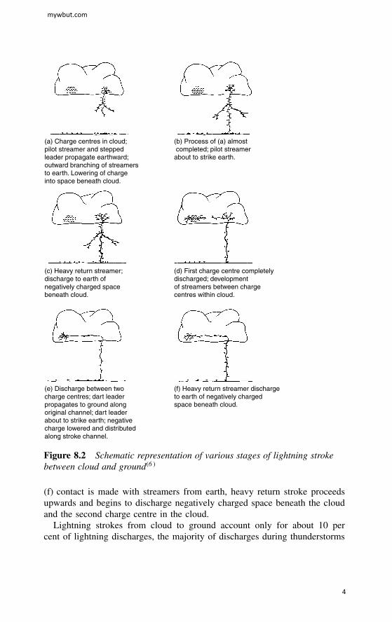
(a) Charge centres in cloud; pilot streamer and steppedleader propagate earthward;outward branching of streamersto earth. Lowering of chargeinto space beneath cloud.

(b) Process of (a) almost completed; pilot streamer about to strike earth.

(c) Heavy return streamer; discharge to earth of negatively charged space beneath cloud.

(d) First charge centre completelydischarged; developmentof streamers between chargecentres within cloud.

(e) Discharge between twocharge centres; dart leaderpropagates to ground along original channel; dart leaderabout to strike earth; negativecharge lowered and distributedalong stroke channel.

(f) Heavy return streamer dischargeto earth of negatively charged space beneath cloud.

Figure 8.2 Schematic representation of various stages of lightning strokebetween cloud and ground�6 �

(f) contact is made with streamers from earth, heavy return stroke proceedsupwards and begins to discharge negatively charged space beneath the cloudand the second charge centre in the cloud.

Lightning strokes from cloud to ground account only for about 10 percent of lightning discharges, the majority of discharges during thunderstorms

mywbut.com

4

take place between clouds. Discharges within clouds often provide generalillumination known as ‘sheath lightning’.

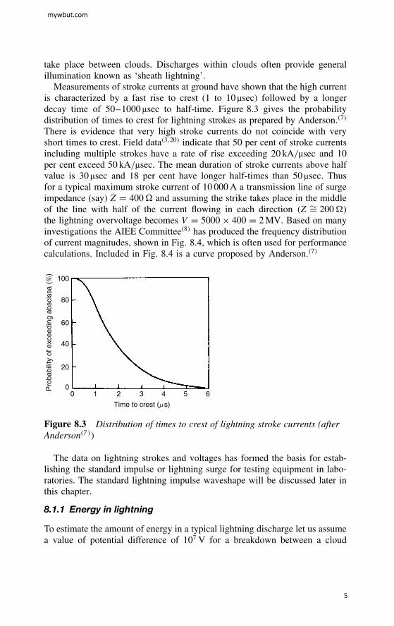
Measurements of stroke currents at ground have shown that the high currentis characterized by a fast rise to crest (1 to 10 µsec) followed by a longerdecay time of 50–1000 µsec to half-time. Figure 8.3 gives the probabilitydistribution of times to crest for lightning strokes as prepared by Anderson.�7�

There is evidence that very high stroke currents do not coincide with veryshort times to crest. Field data�3,20� indicate that 50 per cent of stroke currentsincluding multiple strokes have a rate of rise exceeding 20 kA/µsec and 10per cent exceed 50 kA/µsec. The mean duration of stroke currents above halfvalue is 30 µsec and 18 per cent have longer half-times than 50 µsec. Thusfor a typical maximum stroke current of 10 000 A a transmission line of surgeimpedance (say) Z D 400� and assuming the strike takes place in the middleof the line with half of the current flowing in each direction �Z ¾D 200��the lightning overvoltage becomes V D 5000 ð 400 D 2 MV. Based on manyinvestigations the AIEE Committee�8� has produced the frequency distributionof current magnitudes, shown in Fig. 8.4, which is often used for performancecalculations. Included in Fig. 8.4 is a curve proposed by Anderson.�7�

100

80

60

40

20

00 1 2 3 4

Time to crest (ms)

5 6

Pro

babi

lity

of e

xcee

ding

abs

ciss

a (%

)

Figure 8.3 Distribution of times to crest of lightning stroke currents (afterAnderson�7 ��

The data on lightning strokes and voltages has formed the basis for estab-lishing the standard impulse or lightning surge for testing equipment in labo-ratories. The standard lightning impulse waveshape will be discussed later inthis chapter.

8.1.1 Energy in lightning

To estimate the amount of energy in a typical lightning discharge let us assumea value of potential difference of 107 V for a breakdown between a cloud

mywbut.com

5

0.0510 20 40 60 100 200

0.10.2

0.51

2

5

10

20

40

60

80

90

95

9899

1 2 4 6 10 20

2

Pro

babi

lity

of e

xcee

ding

abs

ciss

a (%

)

Stroke current (kA)

1

1

Figure 8.4 Cumulative distributions of lightning stroke current magnitudes:1. After AIEE Committee.�8 � 2. After Anderson�6 �

and ground and a total charge of 20 coulombs. Then the energy released is20 ð 107 Ws or about 55 kWh in one or more strokes that make the discharge.The energy of the discharge dissipated in the air channel is expended in severalprocesses. Small amounts of this energy are used in ionization of molecules,excitations, radiation, etc. Most of the energy is consumed in the suddenexpansion of the air channel. Some fraction of the total causes heating ofthe struck earthed objects. In general, lightning processes return to the globalsystem the energy that was used originally to create the charged cloud.

8.1.2 Nature of danger

The degree of hazard depends on circumstances. To minimize the chances ofbeing struck by lightning during thunderstorm, one should be sufficiently faraway from tall objects likely to be struck, remain inside buildings or be wellinsulated.

A direct hit on a human or animal is rare; they are more at risk fromindirect striking, usually: (a) when the subject is close to a parallel hit orother tall object, (b) due to an intense electric field from a stroke which can

mywbut.com

6

induce sufficient current to cause death, and (c) when lightning terminating onearth sets up high potential gradients over the ground surface in an outwardsdirection from the point or object struck. Figure 8.5 illustrates qualitativelythe current distribution in the ground and the voltage distribution along theground extending outwards from the edge of a building struck by lightning.�9�

The potential difference between the person’s feet will be largest if his feet areseparated along a radial line from the source of voltage and will be negligibleif he moves at a right angle to such a radial line. In the latter case the personwould be safe due to element of chance.

Vol

tage

0 Distance

(a)

(b)

Figure 8.5 Current distribution and voltage distribution in ground due tolightning stroke to a building (after Golde�9 �)

8.2 Simulated lightning surges for testing

The danger to electric systems and apparatus comes from the potentials thatlightning may produce across insulation. Insulation of power systems may beclassified into two broad categories: external and internal insulation. Externalinsulation is comprised of air and/or porcelain, etc., such as conductor-to-tower clearances of transmission lines or bus supports. If the potential caused

mywbut.com

7

0

1

1 2 3 4 5

Gap spacing (m)

6 7

2

3

4

5

6

Vol

tage

(M

V)

5(−) ms

5(+) ms

CFO(−)CFO(+)

8 m

9.5 m

2(+)

3(+)

2(−) 3(−)

Figure 8.6 Impulse (1.2/50 µsec) flashover characteristics of long rod gapscorrected to STP (after Udo�10 �)

6

5

4

3

2

1

0 10 20 30 40 50

Number of insulators (254 × 146 mm)

Vol

tage

(M

V)

+CFO

−CFO Neg

ativ

e

Pos

itive

µs µs

2

2

3

3

10

105

5

Figure 8.7 Impulse (1.2/50 µsec) flashover characteristics for long insulatorstrings (after Udo�10 �)

mywbut.com

8

by lightning exceeds the strength of insulation, a flashover or puncture occurs.Flashover of external insulation generally does not cause damage to equip-ment. The insulation is ‘self-restoring’. At the worst a relatively short outagefollows to allow replacement of a cheap string of damaged insulation. Internalinsulation most frequently consists of paper, oil or other synthetic insulationwhich insulates h.v. conductors from ground in expensive equipment such astransformers, generators, reactors, capacitors, circuit-breakers, etc. Failure ofinternal insulation causes much longer outages. If power arc follows damageto equipment it may be disastrous and lead to very costly replacements.

The system’s insulation has to be designed to withstand lightning voltagesand be tested in laboratories prior to commissioning.

Exhaustive measurements of lightning currents and voltages and long expe-rience have formed the basis for establishing and accepting what is knownas the standard surge or ‘impulse’ voltage to simulate external or lightningovervoltages. The international standard lightning impulse voltage waveshapeis an aperiodic voltage impulse that does not cross the zero line which reachesits peak in 1.2 µsec and then decreases slowly (in 50 µsec) to half the peakvalue. The characteristics of a standard impulse are its polarity, its peak value,its front time and its half value time. These have been defined in Chapter 2,Fig. 2.23.

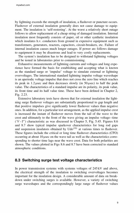
Extensive laboratory tests have shown that for external insulation the light-ning surge flashover voltages are substantially proportional to gap length andthat positive impulses give significantly lower flashover values than negativeones. In addition, for a particular test arrangement, as the applied impulse crestis increased the instant of flashover moves from the tail of the wave to thecrest and ultimately to the front of the wave giving an impulse voltage–time(‘V–T’) characteristic as was discussed in Chapter 5, Fig. 5.45. Figures 8.6and 8.7 show typical impulse sparkover characteristics for long rod gapsand suspension insulators obtained by Udo�10� at various times to flashover.These figures include the critical or long time flashover characteristics (CFO)occurring at about 10 µsec on the wave tail as well as the characteristics corre-sponding to shorter time lags near the wave crest. Data for both polarities areshown. The values plotted in Figs 8.6 and 8.7 have been corrected to standardatmospheric conditions.

8.3 Switching surge test voltage characteristics

In power transmission systems with systems voltages of 245 kV and above,the electrical strength of the insulation to switching overvoltages becomesimportant for the insulation design. A considerable amount of data on break-down under switching surges is available. However, a variety of switchingsurge waveshapes and the correspondingly large range of flashover values

mywbut.com

9

make it difficult to choose a standard shape of switching impulses. Many testshave shown that the flashover voltage for various geometrical arrangementsunder unidirectional switching surge voltages decreases with increasing thefront duration of the surge, reaching the lowest value somewhere in the rangebetween 100 and 500 µsec. The time to half-value has less effect upon thebreakdown strength because flashover almost always takes place before or atthe crest of the wave. Figure 8.8 illustrates a typical relationship for a crit-ical flashover voltage per metre as a function of time to flashover for a 3-mrod-rod gap and a conductor-plane gap respectively.�11� It is seen that the stan-dard impulse voltages give the highest flashover values, with the switchingsurge values of crest between approx. 100 and 500 µsec falling well below thecorresponding power frequency flashover values.

0.6

0.4

0.2

01 10 100 1000

3p.f.

1

2

Time to flashover (µs)

MV

/m

Figure 8.8 Relationship between vertical flashover voltage per metre andtime to flashover (3 m gap). 1. Rod-rod gap. 2. Conductor-plane gap.3. Power frequency

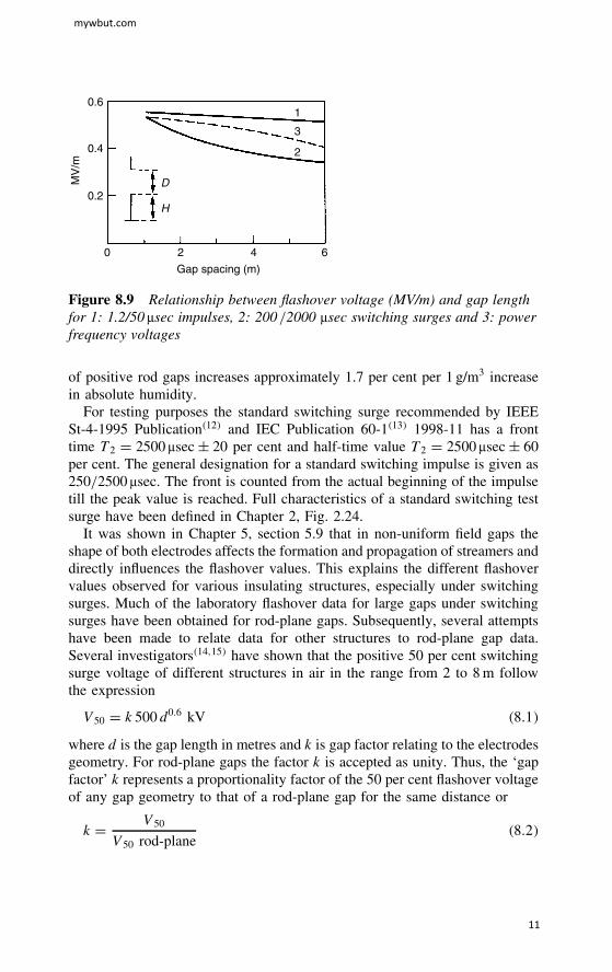
The relative effect of time to crest upon flashover value varies also withthe gap spacing and humidity.�21� Figure 8.9 compares the positive flashovercharacteristics of standard impulses and 200/2000 µsec with power frequencyvoltages for a rod-rod gap plotted as flashover voltage per metre against gapspacing.�11� We observe a rapid fall in switching surge breakdown strengthwith increasing the gap length. This drastic fall in the average switching surgestrength with increasing the insulation length leads to costly design clearances,especially in the ultra-h.v. regions. All investigations show that for nearly allgap configurations which are of practical interest, positive switching impulsesresult in lower flashover voltage than negative ones. The flashover behaviourof external insulations with different configurations under positive switchingimpulse stress is therefore most important. The switching surge voltage break-down is also affected by the air humidity. Kuffel et al.�22� have reported thatover the range from 3 to 16 g/m3 absolute humidity, the breakdown voltage

mywbut.com

10

0.6

0.4

0.2

MV

/m

0 2 4 6

1

2

3

D

H

Gap spacing (m)

Figure 8.9 Relationship between flashover voltage (MV/m) and gap lengthfor 1: 1.2/50 µsec impulses, 2: 200/2000 µsec switching surges and 3: powerfrequency voltages

of positive rod gaps increases approximately 1.7 per cent per 1 g/m3 increasein absolute humidity.

For testing purposes the standard switching surge recommended by IEEESt-4-1995 Publication�12� and IEC Publication 60-1�13� 1998-11 has a fronttime T2 D 2500 µsec š 20 per cent and half-time value T2 D 2500 µsec š 60per cent. The general designation for a standard switching impulse is given as250/2500 µsec. The front is counted from the actual beginning of the impulsetill the peak value is reached. Full characteristics of a standard switching testsurge have been defined in Chapter 2, Fig. 2.24.

It was shown in Chapter 5, section 5.9 that in non-uniform field gaps theshape of both electrodes affects the formation and propagation of streamers anddirectly influences the flashover values. This explains the different flashovervalues observed for various insulating structures, especially under switchingsurges. Much of the laboratory flashover data for large gaps under switchingsurges have been obtained for rod-plane gaps. Subsequently, several attemptshave been made to relate data for other structures to rod-plane gap data.Several investigators�14,15� have shown that the positive 50 per cent switchingsurge voltage of different structures in air in the range from 2 to 8 m followthe expression

V50 D k 500 d0.6 kV �8.1�

where d is the gap length in metres and k is gap factor relating to the electrodesgeometry. For rod-plane gaps the factor k is accepted as unity. Thus, the ‘gapfactor’ k represents a proportionality factor of the 50 per cent flashover voltageof any gap geometry to that of a rod-plane gap for the same distance or

k D V50

V50 rod-plane�8.2�

mywbut.com

11

Expression (8.1) applies to data obtained under the switching impulse ofconstant time to crest. A more general expression which gives minimumstrength and applies to longer times to crest has been proposed by Galletand Leroy�16� as follows:

V50 D k3450

1 C 8

d

kV �8.3�

where k and d have the same meaning as in expression (8.1).In expression (8.2) only the function V50 rod-plane is influenced by the

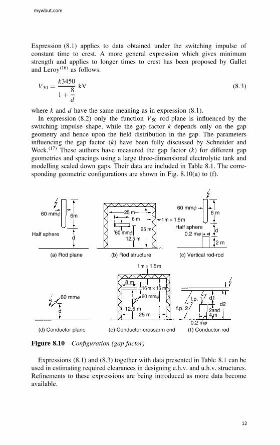
switching impulse shape, while the gap factor k depends only on the gapgeometry and hence upon the field distribution in the gap. The parametersinfluencing the gap factor �k� have been fully discussed by Schneider andWeck.�17� These authors have measured the gap factor �k� for different gapgeometries and spacings using a large three-dimensional electrolytic tank andmodelling scaled down gaps. Their data are included in Table 8.1. The corre-sponding geometric configurations are shown in Fig. 8.10(a) to (f).

Half sphered

6m60 mmf

60 mmf

0.2 mf

0.2 mf

60 mmf60 mmf

60 mmf

(a) Rod plane (b) Rod structure (c) Vertical rod-rod

12.5 m

25 m

25 m6 m 1m × 1.5m

1m × 1.5 m

16m × 16 m

d

6 m

2 m

Half sphere

8 m

12.5 md

(d) Conductor plane (e) Conductor-crossarm end (f) Conductor-rod

f.p. 1 d1

2and4 m

f.p. 225 m

d2

Figure 8.10 Configuration (gap factor)

Expressions (8.1) and (8.3) together with data presented in Table 8.1 can beused in estimating required clearances in designing e.h.v. and u.h.v. structures.Refinements to these expressions are being introduced as more data becomeavailable.

mywbut.com

12

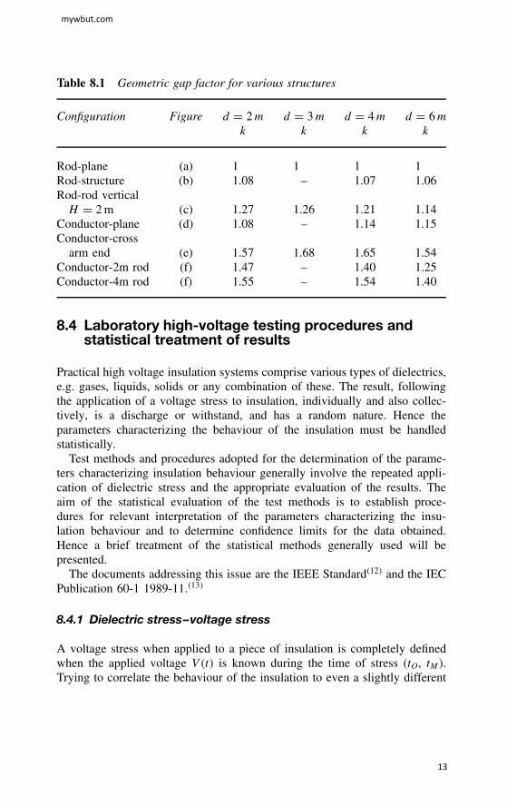
Table 8.1 Geometric gap factor for various structures

Configuration Figure d D 2 m d D 3 m d D 4 m d D 6 mk k k k

Rod-plane (a) 1 1 1 1Rod-structure (b) 1.08 – 1.07 1.06Rod-rod verticalH D 2 m (c) 1.27 1.26 1.21 1.14

Conductor-plane (d) 1.08 – 1.14 1.15Conductor-cross

arm end (e) 1.57 1.68 1.65 1.54Conductor-2m rod (f) 1.47 – 1.40 1.25Conductor-4m rod (f) 1.55 – 1.54 1.40

8.4 Laboratory high-voltage testing procedures andstatistical treatment of results

Practical high voltage insulation systems comprise various types of dielectrics,e.g. gases, liquids, solids or any combination of these. The result, followingthe application of a voltage stress to insulation, individually and also collec-tively, is a discharge or withstand, and has a random nature. Hence theparameters characterizing the behaviour of the insulation must be handledstatistically.

Test methods and procedures adopted for the determination of the parame-ters characterizing insulation behaviour generally involve the repeated appli-cation of dielectric stress and the appropriate evaluation of the results. Theaim of the statistical evaluation of the test methods is to establish proce-dures for relevant interpretation of the parameters characterizing the insu-lation behaviour and to determine confidence limits for the data obtained.Hence a brief treatment of the statistical methods generally used will bepresented.

The documents addressing this issue are the IEEE Standard�12� and the IECPublication 60-1 1989-11.�13�

8.4.1 Dielectric stress–voltage stress

A voltage stress when applied to a piece of insulation is completely definedwhen the applied voltage V�t� is known during the time of stress (tO, tM).Trying to correlate the behaviour of the insulation to even a slightly different

mywbut.com

13

value of V�t� requires accurate knowledge of the physical processes occurringinside the insulation.

8.4.2 Insulation characteristics

The main characteristic of interest of an insulation is the disruptive dischargewhich may occur during the application of stress. However, because of therandomness of the physical processes which lead to disruptive discharge, thesame stress applied several times in the same conditions may not alwayscause disruptive discharge. Also, the discharge when it occurs may occur atdifferent times. In addition, the application of the stress, even if it does notcause discharge, may result in a change of the insulation characteristics.

8.4.3 Randomness of the appearance of discharge

Randomness of the appearance of discharge can be modelled by considering alarge number of stress applications, a fraction p of which causes discharge, D,and the remaining fraction q D �1 � p� being labelled as withstand, W. Thevalue of p depends on applied stress, S, with p D p�S� being the ‘probabilityof discharge’ and it represents one of the characteristics of the insulation.Recognizing that the time to discharge will also vary statistically, the prob-ability of discharge will become a function of both the stress, S, and thetime t.

p�V� D p�t, S� �8.4�

8.4.4 Types of insulation

Insulations are grouped broadly into:

(i) Self-restoring (gases) – no change produced by the application of stressor by discharge, hence the same sample can be tested many times.

(ii) Non-self-restoring (liquids) – affected by discharge only, the same samplecan be used until discharge occurs.

(iii) Affected by applied stress, insulation experiences ageing and in testing itbecomes necessary to introduce a new parameter related to the sequentialapplication of stress.

8.4.5 Types of stress used in high-voltage testing

For design purposes it is sufficient to limit the knowledge of the insulationcharacteristics to a few families of stresses which are a function of time V�t�e.g. switching surge of double exponential with time to crest T1 and to half

mywbut.com

14

value T2 and the variable crest value V (see definitions in Chapter 2 forlightning and switching surges). For testing purposes, the family is furtherrestricted by using fixed times T1 and T2, hence only one variable is left (V).The same applies to both types of surges. The behaviour of the insulationis then defined by the discharge probability as a function of crest voltagep D p�V�.

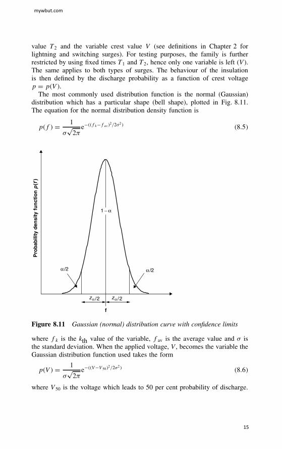
The most commonly used distribution function is the normal (Gaussian)distribution which has a particular shape (bell shape), plotted in Fig. 8.11.The equation for the normal distribution density function is

p�f� D 1

�p

2�e���fk�fav�2/2�2� �8.5�

f

Pro

bab

ility

den

sity

fu

nct

ion

p(f

)

α /2 α /2

zα /2 zα /2

1 − α

Figure 8.11 Gaussian (normal) distribution curve with confidence limits

where fk is the kth value of the variable, fav is the average value and � isthe standard deviation. When the applied voltage, V, becomes the variable theGaussian distribution function used takes the form

p�V� D 1

�p

2�e���V�V50�2/2�2� �8.6�

where V50 is the voltage which leads to 50 per cent probability of discharge.

mywbut.com

15

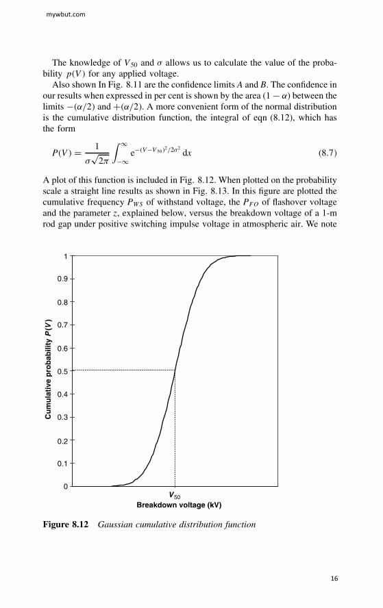
The knowledge of V50 and � allows us to calculate the value of the proba-bility p�V� for any applied voltage.

Also shown In Fig. 8.11 are the confidence limits A and B. The confidence inour results when expressed in per cent is shown by the area (1 � ˛) between thelimits ��˛/2� and C�˛/2�. A more convenient form of the normal distributionis the cumulative distribution function, the integral of eqn (8.12), which hasthe form

P�V� D 1

�p

2�

∫ 1

�1e��V�V50�2/2�2

dx �8.7�

A plot of this function is included in Fig. 8.12. When plotted on the probabilityscale a straight line results as shown in Fig. 8.13. In this figure are plotted thecumulative frequency PWS of withstand voltage, the PFO of flashover voltageand the parameter z, explained below, versus the breakdown voltage of a 1-mrod gap under positive switching impulse voltage in atmospheric air. We note

0

0.1

0.2

0.3

0.4

0.5

0.6

0.7

0.8

0.9

1

Breakdown voltage (kV)

Cu

mu

lati

ve p

rob

abili

ty P

(V)

V50

Figure 8.12 Gaussian cumulative distribution function

mywbut.com

16

0.01

0.05

0.1

0.2

0.5

1

2

5

10

20

30

40

50

60

70

80

90

95

98

99

99.8

99.9

99.9420 440 460 480 500 520 540 560 580 600

Voltage (kV)

0.01

0.05

0.1

0.2

0.5

10

20

30

40

50

60

70

80

90

95

98

99

99.9

99.8

99.9

1

2

5

− 3

− 2

− 1

0

+ 1

+ 2

+ 3

zPfoPws

Figure 8.13 Breakdown voltage distribution plotted on probability scale

that there are three vertical scales, two non-linear giving directly the PWS(l.h.s.), the PFO (r.h.s.) and further to the right a linear scale given in unitsof dimensionless deviation z. The parameter z is convenient for analysis ofnormal distribution results. Equation (8.7) is rewritten in the form

P�z� D 1

�p

2�

∫ z

�1e��z2/2� dz �8.8�

mywbut.com

17

where

z D V� V50

�

As noted earlier the distribution of flashover of the gap is characterized bytwo parameters:

(i) V50, called the critical flashover (CFO),(ii) �, called the standard deviation.

Both can be read directly from the best fit line drawn through the exper-imentally determined points. Note, that CFO corresponds to z D 0 and � isgiven by the difference between two consecutive integers of z. In practice thevoltage range over which the probability of flashover is distributed is

CFO š 3� �8.9�

ž (CFO � 3�) is known as the statistical withstand voltage (SWV) and repre-sents the point with flashover probability 0.13 per cent;

ž (CFO C 3�) is known as the statistical flashover voltage (SFOV) and repre-sents the point with flashover probability 99.87 per cent.

The SWV and SFOV are used in insulation coordination and will bediscussed later. For a complete description of insulation parameters, thetime to breakdown must also be considered. The times to breakdown arerepresented by

P�t� D 1

�p

2�

∫ t

0e��t�t�2/2�2

dt �8.10�

where

t D mean time to breakdown,� D standard deviation.

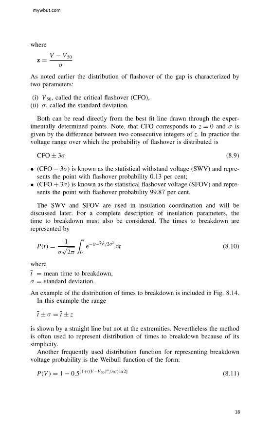
An example of the distribution of times to breakdown is included in Fig. 8.14.In this example the range

t š � D t š z

is shown by a straight line but not at the extremities. Nevertheless the methodis often used to represent distribution of times to breakdown because of itssimplicity.

Another frequently used distribution function for representing breakdownvoltage probability is the Weibull function of the form:

P�V� D 1 � 0.5[1C��V�V50�m/n�� ln 2] �8.11�

mywbut.com

18

0.01

0.05

0.1

0.2

0.5

1

2

5

10

20

30

40

50

60

70

80

90

95

98

99

99.8

99.9

99.9 0.01

0.050.1

0.2

0.5

1

2

5

10

20

30

40

50

60

70

80

90

95

98

99

99.8

99.9

99.9

420 200 300 400 500

z = + 1

z

z = 0

z = −1

Time to breakdown (µs)

P

Figure 8.14 Distribution of times to breakdown

where

P�V� D the probability of flashover,V D the applied voltage,V50 D the applied voltage which gives 50 per cent probability flashover,� D the standard deviation.

In the Weibull function n is not known but it determines the voltage V50 � n�below which no flashover occurs, or P�V� D 0 for V � V50 � n�. For air n

mywbut.com

19

lies in the range 3 � n � 4. The value 3 is usually used resulting in

m Dln

ln 0.84

ln 0.5

lnn� 1

n

D 3.4 �8.12�

The adaptation of the Weibull function to normal distribution using the abovevalues for n and m gives P�V� D 0.5 for V D V50 and P�V� D 0.16 for V DV50 � �. Both the Gaussian and the Weibull functions give the same resultsin the range 0.01 � P�V� � 0.99.

8.4.6 Errors and confidence in results

In the determination of a parameter two types of error are present:

(i) error associated with the statistical nature of the phenomena and thelimited number of tests (εS),

(ii) error in the measurement (εM).

The statistical error is expressed by means of two confidence limits C percent. The total error is given by

εT D√ε2M C ε2

S �8.13�

The various IEC recommendations specify the permissible measurement accu-racy as 3 per cent. Hence, a statistical error of, say, 2 per cent will increasethe total error by a factor of 1.2, while a statistical error of 1.5 per cent willincrease the total error by 1.1.

The outcome of a test procedure and the analysis of the results is usuallyan average of a parameter z with C per cent confidence limits zA and zB (seeFig. 8.11). For a normal distribution the probability density of a function fora frequency of occurrence can be represented graphically in terms of area asshown in Fig. 8.11 (1 � ˛).

8.4.7 Laboratory test procedures

The test procedures applied to various types of insulation are describedin national and international standards as already mentioned before.�12,13�

Because the most frequently occurring overvoltages on electric systemsand apparatus originate in lightning and switching overvoltages, mostlaboratory tests are conducted under standard lightning impulse voltagesand switching surge voltages. Three general testing methods have beenaccepted:

mywbut.com

20

1. Multi-level method.2. Up and down method.3. Extended up and down method.

1. Multi-level test method

In this method the procedure is:

ž choose several test voltage levels,ž apply a pre-specified number of shots at each level (n),ž count the number (x) of breakdowns at each voltage level,ž plot p�V� (xj/n) against V (kV),ž draw a line of best fit on a probability scale,ž from the line determine V50 at z D 0 or P�V� D 50 per cent,ž and � at z D 1 or � D V50% � V16%

P(V)

kV

Figure 8.15 Probability of breakdown distribution using the multi-levelmethod

The recorded probability of breakdown, xj/n, is the number which resultedin breakdown from the application of n shots at voltage Vj. When xj/n isplotted against Vj on a linear probability paper a straight line is obtained asshown in Fig. 8.15.

The advantage of this method is that it does not assume normality ofdistribution. The disadvantage is that it is time consuming, i.e. many shotsare required.

This test method is generally preferred for research and live-line testing(typically 100 shots per level, with 6–10 levels).

2. Up and down method

In this method a starting voltage (Vj) close to the anticipated flashover value isselected. Then equally spaced voltage levels (V) above and below the starting

mywbut.com

21

voltage are chosen. The first shot is applied at the voltage Vj. If breakdownoccurs the next shot is applied at Vj �V. If the insulation withstands, thenext voltage is applied at Vj CV. The sequential procedure of testing isillustrated in Fig. 8.16.

Figure 8.17 illustrates the sequence with nine shots applied to the insulationunder test. The IEC Standard for establishing V50 (50 per cent) withstandvoltage requires a minimum n D 20 voltage applications for self-restoring

Pick startingvoltage V1 = Vi

Pick ∆V

Apply one shotat Vi

Breakdown Withstand

Apply next shotat Vi − ∆V

Apply next shotat Vi + ∆V

Figure 8.16 Schematics of the sequential up and down procedure

∆V

Vo

1

2

3

4

5

6

7

8

9

breakdown

withstand

Vo = lowest level at which a shot is applied

Figure 8.17 Example illustrating the application of nine shots in thesequential up and down method. X D breakdown; O D withstand

mywbut.com

22

insulation. To evaluate the V10 (10 per cent) withstand voltage for self-restoring insulation with the up and down method with one impulse per groupalso requires a minimum of n D 20 applications.

In practice the points, expressing the probability of withstand, are plottedagainst the voltage Vj on a probability scale graph as was shown in Fig. 8.13.The best straight line is then plotted using curve fitting techniques. The 50per cent and 10 per cent discharge voltages are obtained directly from thegraph. This method has the advantage that it requires relatively few shotsand therefore is most frequently used by industry. The disadvantage is that itassumes normality and is not very accurate in determining �. Alternatively,the V10 can be obtained from the V50 using the formula

V10 D V50�1 � 1.3z� D V50 Ð 0.96 �8.14�

From the sequentially obtained readings (Fig. 8.17), the values of V50 and� can be also calculated analytically as follows.

In the example chosen (Fig. 8.17): total number of shots n D 9, total numberof breakdowns nb D 4, total number of withstands nw D 5, and lowest levelat which a shot is applied D V0.

In calculating V50% and �,

if nb > nw then ni D number of withstands at level j

if nw > nb then nj D number of breakdowns at level j

(always use the smaller of the two). The expressions are:

V50 D V0 CV

[A

Nš 1

2

]){ni D nbi use negative signni D nwi use positive sign

�8.15�

� D 1.62AV

(NB� A2

N2 C 0.029

)�8.16�

where

N Dk∑iD0

niw ork∑iD0

nib

A Dk∑iD0

iniw ork∑iD0

inib

B Dk∑iD0

i2niw ork∑iD0

i2nib

with i referring to the voltage level, niw to the number of withstands and nibthe number of breakdowns at that level.

mywbut.com

23

3. The extended up and down method

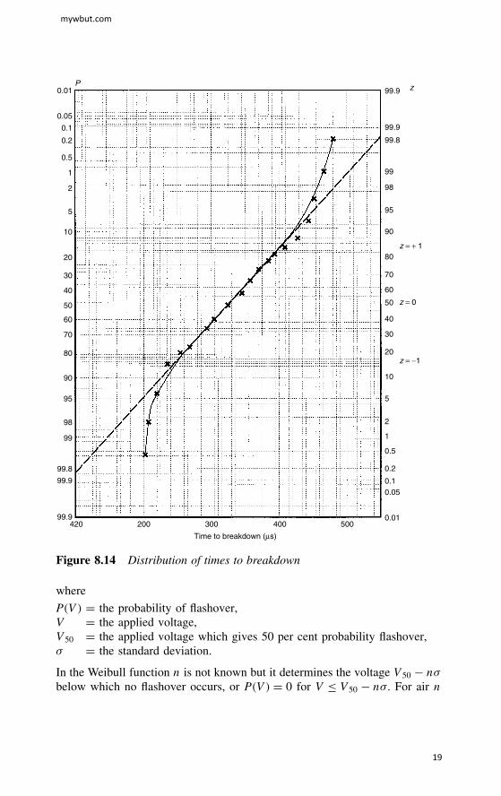
This method is also used in testing self-restoring insulation. It can be used todetermine discharge voltages corresponding to any probability p. A numberof impulses are applied at a certain voltage level. If none causes discharge,the voltage is increased by a step V and the impulses are applied until atleast one causes breakdown, then the voltage is decreased. For an example ofthe extended up and down method procedure see Fig. 8.18.

07

07

07

11

07

12

13

07

07

07

14

12

12

07

17

940

970

1000

1030

1060

Figure 8.18 Example of the extended up and down method

The number n is determined such that a series of n shots would have 50 percent probability of giving at least one flashover. The 50 per cent probabilityof discharge is given by

0.5 D 1 � �1 � p�n

or

n D 0.5 D ln �1 � p� �8.17�

from which p becomes a discrete value. The value n D 7 impulses per voltagelevel is often used as it allows the determination of 10 per cent dischargevoltage without the necessity to use �. Substituting n D 7 into eqn (8.17)gives p D 0.094 or approximately 10 per cent.

The IEC switching withstand voltage is defined as 10 per cent withstand,hence the extended up and down method has an advantage. Other advantagesinclude: discharge on test object is approximately 10 per cent the number ofapplied impulses rather than 50 per cent as applicable to the up and down

mywbut.com

24

method. Also the highest voltage applied is about V50 rather than V50 C 2. Inthe up and down method the V10% may also be obtained from:

V10 D V50 �1 � 1.13z� D V50 Ð 0.96 �8.18�

In today’s power systems for voltages up to 245 kV insulation tests are stilllimited to lightning impulses and the one-minute power frequency test. Above300 kV, in addition to lightning impulses and the one-minute power frequencytests, tests include the use of switching impulse voltages.

8.4.8 Standard test procedures

1. Proof of lightning impulse withstand level

For self-restoring insulation the test procedures commonly used for withstandestablishment are:

(i) 15 impulses of rated voltage and of each polarity are applied, up to twodisruptive discharges are permitted,

(ii) in the second procedure the 50 per cent flashover procedure using eitherthe up and down or extended up and down technique as described earlier.

From the up and down method the withstand voltage is obtained usingeqn (8.18). In tests on non-self-restoring insulation, three impulses are appliedat the rated withstand voltage level of a specified polarity. The insulation isdeemed to have withstood if no failure is observed.

2. Testing with switching impulses

These tests apply for equipment at voltages above 300 kV. The testingprocedure is similar to lightning impulses using 15 impulses. The tests arecarried out in dry conditions while outdoor equipment is tested under positiveswitching impulses only. In some cases, when testing circuit isolators or circuitbreakers which may experience combined voltage stress (power frequencyand switching surge) biased tests using combined power frequency and surgevoltages are used. The acceptable insulating capability requires 90 per centwithstand capability.

8.4.9 Testing with power frequency voltage

The standard practice requires the insulation to perform a one-minute test withpower frequency at a voltage specified in the standards. For indoor equipment,the equipment is tested in dry conditions, while outdoor equipment is testedunder prescribed rain conditions for which IEC prescribes a precipitation rateof 1–1.5 mm/min with resistivity of water.

mywbut.com

25

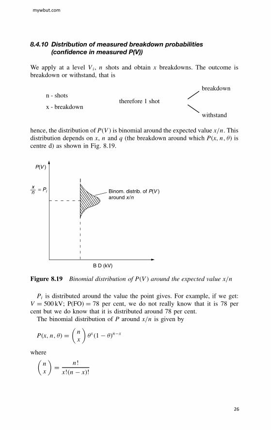
8.4.10 Distribution of measured breakdown probabilities(confidence in measured P(V))

We apply at a level Vi, n shots and obtain x breakdowns. The outcome isbreakdown or withstand, that is

n - shots

x - breakdowntherefore 1 shot

breakdown

withstand

hence, the distribution of P�V� is binomial around the expected value x/n. Thisdistribution depends on x, n and q (the breakdown around which P�x, n, +� iscentre d) as shown in Fig. 8.19.

Binom. distrib. of P(V )around x/n

P(V )

= Pixn

I

B D (kV)

Figure 8.19 Binomial distribution of P�V� around the expected value x/n

Pi is distributed around the value the point gives. For example, if we get:V D 500 kV; P(FO) D 78 per cent, we do not really know that it is 78 percent but we do know that it is distributed around 78 per cent.

The binomial distribution of P around x/n is given by

P�x, n, +� D(nx

)+x�1 � +�n�x

where(nx

)D n!

x!�n� x�!

mywbut.com

26

+ D true value of the most likely outcome (value around which the distributionis centred).

We do not know + but we can replace it with the expected value x/n aswas shown in Fig. 8.19.

Hence

P�x, n, +� D(nx

)+x�1 � +� �8.19�

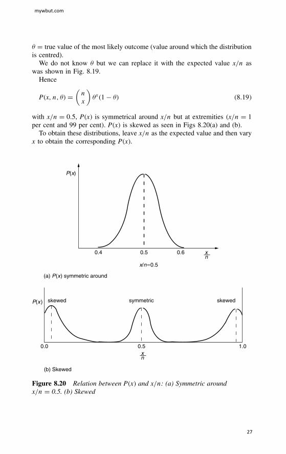
with x/n D 0.5, P�x� is symmetrical around x/n but at extremities �x/n D 1per cent and 99 per cent). P�x� is skewed as seen in Figs 8.20(a) and (b).

To obtain these distributions, leave x/n as the expected value and then varyx to obtain the corresponding P�x�.

P(x)

P(x)

skewed skewedsymmetric

0.0 0.5 1.0xn

0.4 0.5 0.6 xn

(a) P(x) symmetric around

(b) Skewed

x/n=0.5

Figure 8.20 Relation between P�x� and x/n: (a) Symmetric aroundx/n D 0.5. (b) Skewed

mywbut.com

27

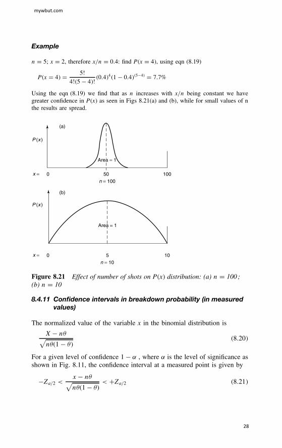
Example

n D 5; x D 2, therefore x/n D 0.4: find P�x D 4�, using eqn (8.19)

P�x D 4� D 5!

4!�5 � 4�!�0.4�4�1 � 0.4��5�4� D 7.7%

Using the eqn (8.19) we find that as n increases with x/n being constant we havegreater confidence in P�x� as seen in Figs 8.21(a) and (b), while for small values of nthe results are spread.

0x =

(a)

(b)

P (x )

P (x )

50n = 100

100

0x = 5n = 10

10

Area = 1

Area = 1

Figure 8.21 Effect of number of shots on P�x� distribution: (a) n D 100 ;(b) n D 10

8.4.11 Confidence intervals in breakdown probability (in measuredvalues)

The normalized value of the variable x in the binomial distribution is

X� n+√n+�1 � +�

�8.20�

For a given level of confidence 1 � ˛ , where ˛ is the level of significance asshown in Fig. 8.11, the confidence interval at a measured point is given by

�Za/2 < x � n+√n+�1 � +�

< CZa/2 �8.21�

mywbut.com

28

The probability of breakdown with a confidence level 1 � ˛ is given by

P�V� D x

nš Za/2

√√√√ x

n

(1 � x

n

)n

�8.22�

Using this expression it can be shown on the linear probability scale that theconfidence in the measured values of breakdown is at maximum at x/n D 0.5and progressively decreases as the extreme values of breakdown probabilityare approached. Za/2 is obtained from tables of statistics or for conveniencefrom the graph directly.

Example

n D 10; x D 5 for a confidence level of 90 per cent

˛ D 1 � 0.9 D 0.1

using statistical tables,�25� we obtain for

a

2D 0.05, Za/2 D 1.64

hence

P�V� D 12 š �1.64�

√12

(12

)10

The confidence limit at near P�V� D 50 per cent is much smaller than theconfidence limit for P�V� approaching 1 per cent or 99 per cent. The solutionis a non-linear distribution of n, that is we need to take many shots near thelimits and a few in the middle. Confidence expressed in terms of kV is moreconvenient than confidence in probability as shown in Fig. 8.22.

P(V )

V50

∆V

∆Z

kV

Z

Z = 1

Z = 0

Z = −1

50%23%

Figure 8.22 Confidence expressed in kV

mywbut.com

29

Using the same example as before

23% � P�V50� � 77%

to determine z D z1 � z2

z1 is determined from the value of P(0.50)

z2 is determined from the value of P(0.23)

from Fig. 8.22

for F�z� D 50% D 0.5, z1 D 0.0

for F�z� D 23% D �0.77, z2 D �0.74

therefore

z D z1 � z2

D 0 � ��0.74�

D 0.74

the standard deviation � is the run from z D 0 to z D 1 therefore

rise D slope

D z/V

D 1/�

and therefore V D z�Thus the confidence in V is

V D VšV

D Všz� �8.23�

confidence in

V50 D V50 š �0.74�� �8.24�

8.5 Weighting of the measured breakdown probabilities

Weights can be assigned to various data points to the measured breakdownprobability and the number of impulses applied at each level.

8.5.1 Fitting of the best fit normal distribution

On probability paper the normal distribution best characterizing the data pointswill appear as the best fit straight line. An example of this is shown inFig. 8.23.

mywbut.com

30

450 500 550 600 650

V1

Breakdown voltage (kV)

ZIzi

Z(v)z = +3

z = +2

z = +1

z = +0

z = −1

z = −2

z = −3

Figure 8.23 Best fit normal distribution drawn through measured flashoverprobability points

In order to obtain this best fit straight line, it is necessary to minimize thedeviation of the data points around the line. The root mean square deviationfor the case shown in Fig. 8.23 is given by√

1

m

∑iD1

wi �zi � .i�2 �8.25�

where xi is the value of the measured breakdown probability on the probitscale at the voltage level Vi, xi is the probit scale value of the breakdownprobability as given by the best fit straight line for the same voltage level, andw1 is the weighting coefficient assigned to the measurement, xi. The expressiongiven in eqn (8.25) is in terms of the dimensionless deviation z. This can berewritten using

zi D Vi � V50

��8.26�

to obtain√√√√ 1

m

∑iD1

wi

(Vi � V50

�� .i

)2

�8.27�

mywbut.com

31

Minimizing this expression is equivalent to minimizing

∑iD1

wi

(Vi � V50

�� .i

)2

�8.28�

The minimum value of the above expression occurs when the quantity∑iD1

wi �Vi � V50 � �.i�2 �8.29�

is at its minimum. The best fit straight line which is in fact the normal distri-bution best representing the breakdown probability can now be obtained bysetting

∂

∂V50

∑iD1

wi �Vi � V50 � �.i�2 D 0 �8.30�

and

∂

∂�∑iD1

wi �Vi � V50 � �.i�2 D 0 �8.31�

and solving for V50 and �. These values are found by carrying out the partialdifferentiation of eqns (8.30) and (8.31). This gives the following two simul-taneous equations∑

iD1

wi vi �∑iD1

wiV50 � �∑iD1

wi.i D 0 �8.32�

and∑iD1

wiVi.i � V50

∑iD1

wi.i � �∑iD1

wi.2i D 0 �8.33�

which can be solved to obtain

V50 D

∑iD1

wiVi � �∑iD1

wi.i

∑iD1

wi�8.34�

and

� D

∑iD1

wiVi∑iD1

wi.i �∑iD1

wi∑iD1

wiVi.i

(∑iD1

wi.i

)2

�∑iD1

wi∑iD1

wi.2i

�8.35�

Thus values for V50 and � are obtained.

mywbut.com

32

8.6 Insulation coordination

Insulation coordination is the correlation of insulation of electrical equip-ment with the characteristics of protective devices such that the insulationis protected from excessive overvoltages. In a substation, for example, theinsulation of transformers, circuit breakers, bus supports, etc., should haveinsulation strength in excess of the voltage provided by protective devices.

Electric systems insulation designers have two options available to them:(i) choose insulation levels for components that would withstand all kinds ofovervoltages, (ii) consider and devise protective devices that could be installedat the sensitive points in the system that would limit overvoltages there. Thefirst alternative is unacceptable especially for e.h.v. and u.h.v. operating levelsbecause of the excessive insulation required. Hence, there has been great incen-tive to develop and use protective devices. The actual relationship between theinsulation levels and protective levels is a question of economics. Conventionalmethods of insulation coordination provide a margin of protection betweenelectrical stress and electrical strength based on predicted maximum over-voltage and minimum strength, the maximum strength being allowed by theprotective devices.

8.6.1 Insulation level

‘Insulation level’ is defined by the values of test voltages which the insulationof equipment under test must be able to withstand.

In the earlier days of electric power, insulation levels commonly used wereestablished on the basis of experience gained by utilities. As laboratory tech-niques improved, so that different laboratories were in closer agreement ontest results, an international joint committee, the Nema-Nela Committee onInsulation Coordination, was formed and was charged with the task of estab-lishing insulation strength of all classes of equipment and to establish levels forvarious voltage classification. In 1941 a detailed document�18� was publishedgiving basic insulation levels for all equipment in operation at that time.The presented tests included standard impulse voltages and one-minute powerfrequency tests.

In today’s systems for voltages up to 245 kV the tests are still limitedto lightning impulses and one-minute power frequency tests, see section 8.3.Above 300 kV, in addition to lightning impulse and the one-minute powerfrequency tests, tests include the use of switching impulse voltages. Tables 8.2and 8.3 list the standardized test voltages for �245 kV and above ½300 kVrespectively, suggested by IEC for testing equipment. These tables are basedon a 1992 draft of the IEC document on insulation coordination.

mywbut.com

33

Table 8.2 Standard insulation levels for Range I (1 kV < Um � 245 kV)(From IEC document 28 CO 58, 1992, Insulation coordination Part 1:definitions, principles and rules)

Highest voltage Standard Standardfor equipment power frequency lightning impulse

Um short-duration withstand voltagekV withstand voltage kV

(r.m.s. value) kV (peak value)(r.m.s. value)

3.6 10 2040

7.2 20 4060

12 28 607595

17.5 38 7595

24 50 95125145

36 70 145170

52 95 25072.5 140 325

123 (185) 450230 550

145 (185) (450)230 550275 650

170 (230) (550)257 650325 750

245 (275) (650)(325) (750)360 850395 950460 1050

mywbut.com

34

Table 8.3 Standard insulation levels for Range II (Um > 245 kV) (FromIEC document 28 CO 58, 1992, Insulation coordination Part 1: definitions,principles and rules)

Highest Longitudinal Standard Phase-to-phase Standardvoltage for insulation lightning (ratio to the lightningequipment �C� kV impulse phase-to-earth impulseUm kV (peak value) withstand voltage peak withstand

(r.m.s. value) Phase-to-earth value) voltage kVkV (peak value)

(peak value)

300 750 750 1.50 850950

750 850 1.50 9501050

362 850 850 1.50 9501050

850 950 1.50 10501175

420 850 850 1.60 10501175

950 950 1.50 11751300

950 1050 1.50 13001425

525 950 950 1.70 11751300

950 1050 1.60 13001425

950 1175 1.50 14251550

765 1175 1300 1.70 16751800

1175 1425 1.70 18001950

1175 1550 1.60 19502100

�C�Value of the Impulse component of the relevant combined test.Note: The introduction of Um D 550 kV (instead of 525 kV), 800 kV (instead of 765 kV), 1200 kV, of a value between 765 kVand the associated standard withstand voltages, are under consideration.

mywbut.com

35

8.6.2 Statistical approach to insulation coordination

In the early days insulation levels for lightning surges were determined byevaluating the 50 per cent flashover values (BIL) for all insulations andproviding a sufficiently high withstand level that all insulations would with-stand. For those values a volt– time characteristic was constructed. Similarlythe protection levels provided by protective devices were determined. The twovolt– time characteristics are shown in Fig. 8.24. The upper curve representsthe common BIL for all insulations present, while the lower represents theprotective voltage level provided by the protective devices. The differencebetween the two curves provides the safety margin for the insulation system.Thus the

Protection ratio D Max. voltage it permits

Max. surge voltage equipment withstands�8.36�

kV

A

B

time

A: protecting device

B: device to be protected

safety margin

Figure 8.24 Coordination of BILs and protection levels (classical approach)

This approach is difficult to apply at e.h.v. and u.h.v. levels, particularly forexternal insulations.

Present-day practices of insulation coordination rely on a statistical approachwhich relates directly the electrical stress and the electrical strength.�11� Thisapproach requires a knowledge of the distribution of both the anticipatedstresses and the electrical strengths.

mywbut.com

36

The statistical nature of overvoltages, in particular switching overvoltages,makes it necessary to compute a large number of overvoltages in order todetermine with some degree of confidence the statistical overvoltages on asystem. The e.h.v. and u.h.v. systems employ a number of non-linear elements,but with today’s availability of digital computers the distribution of overvolt-ages can be calculated. A more practical approach to determine the requiredprobability distributions of a system’s overvoltages employs a comprehen-sive systems simulator, the older types using analogue units, while the neweremploy real time digital simulators (RTDS).�24�

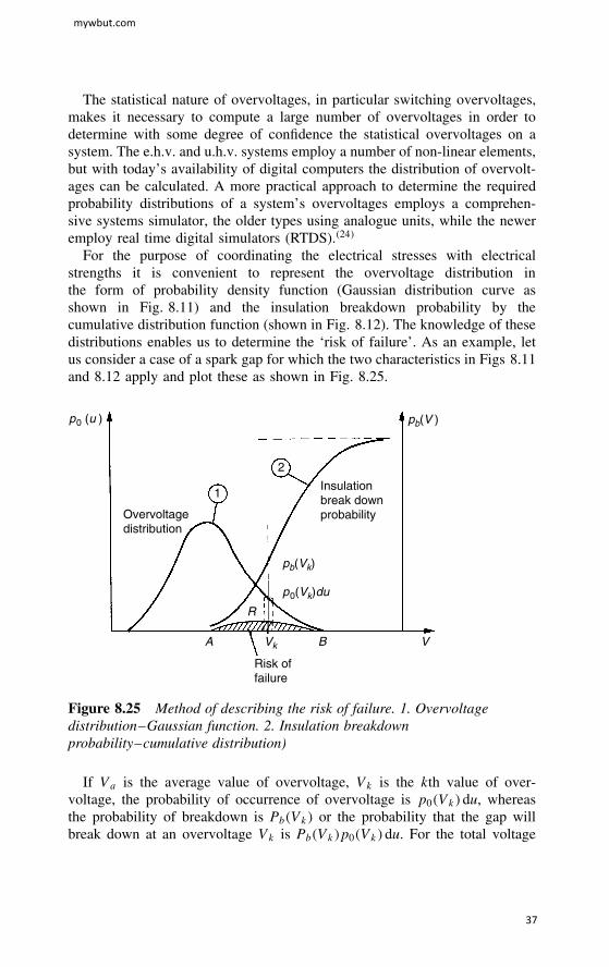
For the purpose of coordinating the electrical stresses with electricalstrengths it is convenient to represent the overvoltage distribution inthe form of probability density function (Gaussian distribution curve asshown in Fig. 8.11) and the insulation breakdown probability by thecumulative distribution function (shown in Fig. 8.12). The knowledge of thesedistributions enables us to determine the ‘risk of failure’. As an example, letus consider a case of a spark gap for which the two characteristics in Figs 8.11and 8.12 apply and plot these as shown in Fig. 8.25.

Overvoltagedistribution

1

2

Insulationbreak downprobability

pb(Vk)

pb(V )

p0(Vk)du

p0 (u )

R

A B VVk

Risk offailure

Figure 8.25 Method of describing the risk of failure. 1. Overvoltagedistribution–Gaussian function. 2. Insulation breakdownprobability–cumulative distribution)

If Va is the average value of overvoltage, Vk is the kth value of over-voltage, the probability of occurrence of overvoltage is p0�Vk� du, whereasthe probability of breakdown is Pb�Vk� or the probability that the gap willbreak down at an overvoltage Vk is Pb�Vk�p0�Vk� du. For the total voltage

mywbut.com

37

range we obtain for the total probability of failure or ‘risk of failure’

R D∫ 1

0Pb�Vk�p0�Vk� du. �8.37�

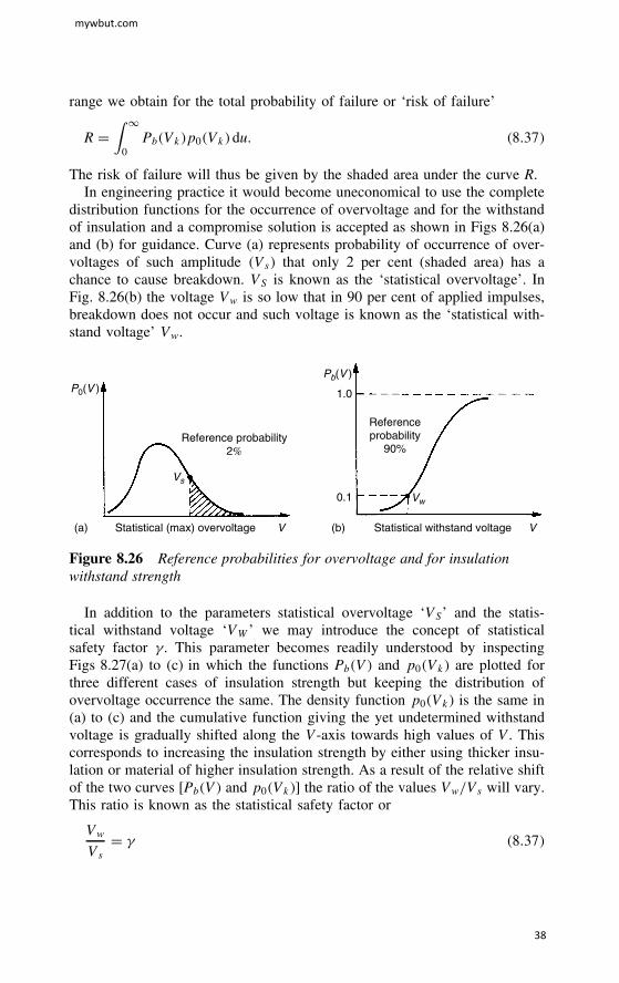
The risk of failure will thus be given by the shaded area under the curve R.In engineering practice it would become uneconomical to use the complete

distribution functions for the occurrence of overvoltage and for the withstandof insulation and a compromise solution is accepted as shown in Figs 8.26(a)and (b) for guidance. Curve (a) represents probability of occurrence of over-voltages of such amplitude �Vs� that only 2 per cent (shaded area) has achance to cause breakdown. VS is known as the ‘statistical overvoltage’. InFig. 8.26(b) the voltage Vw is so low that in 90 per cent of applied impulses,breakdown does not occur and such voltage is known as the ‘statistical with-stand voltage’ Vw.

P0(V )Pb(V )

Reference probability2%

Vs

Statistical (max) overvoltage V Statistical withstand voltage V

1.0

0.1 Vw

Referenceprobability

90%

(a) (b)

Figure 8.26 Reference probabilities for overvoltage and for insulationwithstand strength

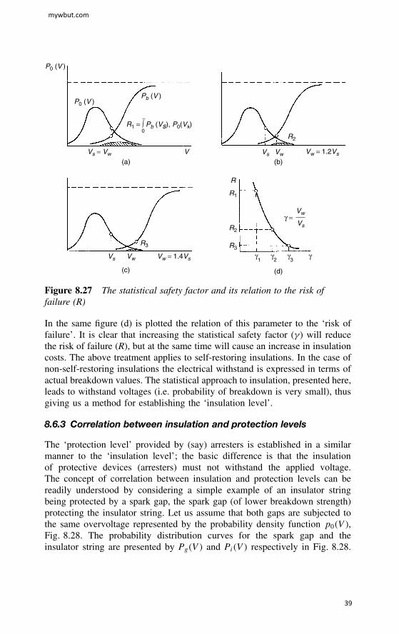
In addition to the parameters statistical overvoltage ‘VS’ and the statis-tical withstand voltage ‘VW’ we may introduce the concept of statisticalsafety factor 4 . This parameter becomes readily understood by inspectingFigs 8.27(a) to (c) in which the functions Pb�V� and p0�Vk� are plotted forthree different cases of insulation strength but keeping the distribution ofovervoltage occurrence the same. The density function p0�Vk� is the same in(a) to (c) and the cumulative function giving the yet undetermined withstandvoltage is gradually shifted along the V-axis towards high values of V. Thiscorresponds to increasing the insulation strength by either using thicker insu-lation or material of higher insulation strength. As a result of the relative shiftof the two curves [Pb�V� and p0�Vk�] the ratio of the values Vw/Vs will vary.This ratio is known as the statistical safety factor or

VwVs

D 4 �8.37�

mywbut.com

38

P0 (V )

P0 (V )Pb (V )

(a) (b)

(c) (d)

Vs = Vw Vs Vw

Vs Vw

Vw = 1.2Vs

Vw = 1.4Vs

V

R1 = ∫ Pb (Vs), P0(Vk)0

R2

R3

R1

R

R2

R3

Vs

Vwγ =

γ1

γ2

γ3

γ

Figure 8.27 The statistical safety factor and its relation to the risk offailure (R)

In the same figure (d) is plotted the relation of this parameter to the ‘risk offailure’. It is clear that increasing the statistical safety factor (4) will reducethe risk of failure (R), but at the same time will cause an increase in insulationcosts. The above treatment applies to self-restoring insulations. In the case ofnon-self-restoring insulations the electrical withstand is expressed in terms ofactual breakdown values. The statistical approach to insulation, presented here,leads to withstand voltages (i.e. probability of breakdown is very small), thusgiving us a method for establishing the ‘insulation level’.

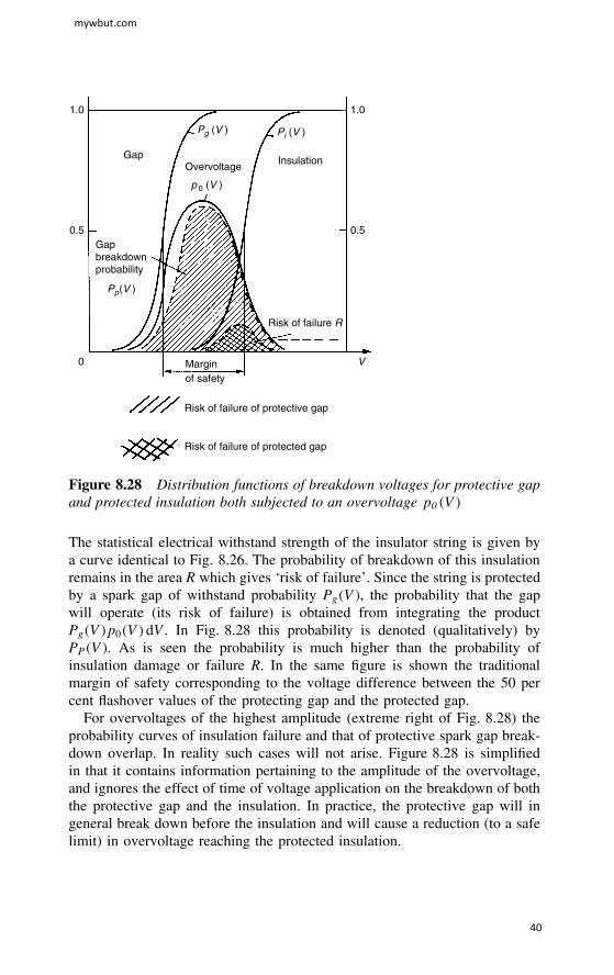
8.6.3 Correlation between insulation and protection levels

The ‘protection level’ provided by (say) arresters is established in a similarmanner to the ‘insulation level’; the basic difference is that the insulationof protective devices (arresters) must not withstand the applied voltage.The concept of correlation between insulation and protection levels can bereadily understood by considering a simple example of an insulator stringbeing protected by a spark gap, the spark gap (of lower breakdown strength)protecting the insulator string. Let us assume that both gaps are subjected tothe same overvoltage represented by the probability density function p0�V�,Fig. 8.28. The probability distribution curves for the spark gap and theinsulator string are presented by Pg�V� and Pi�V� respectively in Fig. 8.28.

mywbut.com

39

Gapbreakdownprobability

Marginof safety

Risk of failure of protective gap

Risk of failure R

Risk of failure of protected gap

1.0

Gap

Pg (V )

p 0 (V )

Pi (V )

OvervoltageInsulation

0.5

1.0

0.5

0 V

Pp(V )

Figure 8.28 Distribution functions of breakdown voltages for protective gapand protected insulation both subjected to an overvoltage p0 �V�

The statistical electrical withstand strength of the insulator string is given bya curve identical to Fig. 8.26. The probability of breakdown of this insulationremains in the area R which gives ‘risk of failure’. Since the string is protectedby a spark gap of withstand probability Pg�V�, the probability that the gapwill operate (its risk of failure) is obtained from integrating the productPg�V�p0�V� dV. In Fig. 8.28 this probability is denoted (qualitatively) byPP�V�. As is seen the probability is much higher than the probability ofinsulation damage or failure R. In the same figure is shown the traditionalmargin of safety corresponding to the voltage difference between the 50 percent flashover values of the protecting gap and the protected gap.

For overvoltages of the highest amplitude (extreme right of Fig. 8.28) theprobability curves of insulation failure and that of protective spark gap break-down overlap. In reality such cases will not arise. Figure 8.28 is simplifiedin that it contains information pertaining to the amplitude of the overvoltage,and ignores the effect of time of voltage application on the breakdown of boththe protective gap and the insulation. In practice, the protective gap will ingeneral break down before the insulation and will cause a reduction (to a safelimit) in overvoltage reaching the protected insulation.

mywbut.com

40

8.7 Modern power systems protection devices

8.7.1 MOA – metal oxide arresters

The development of MOA (metal oxide arresters) represented a breakthroughin overvoltage protection devices. It became possible to design arresterswithout using gaps which were indispensable in the conventional lightningarresters, which utilized non-linear resistors made of silicon Carbide (SiC)and spark gaps. Figure 8.29 shows a block diagram of the valve arrangementsin the two types of arrester.

In (a) the elements and the spark gaps are connected in series. In (b) theelements are stacked on top of each other without the need for spark gaps.

H.V.

SiC elements

Spark gaps

H.V.

MO elements

(a)

(b)

Figure 8.29 Block diagram of valve arrangements in (a) SiC, (b) MOA

mywbut.com

41

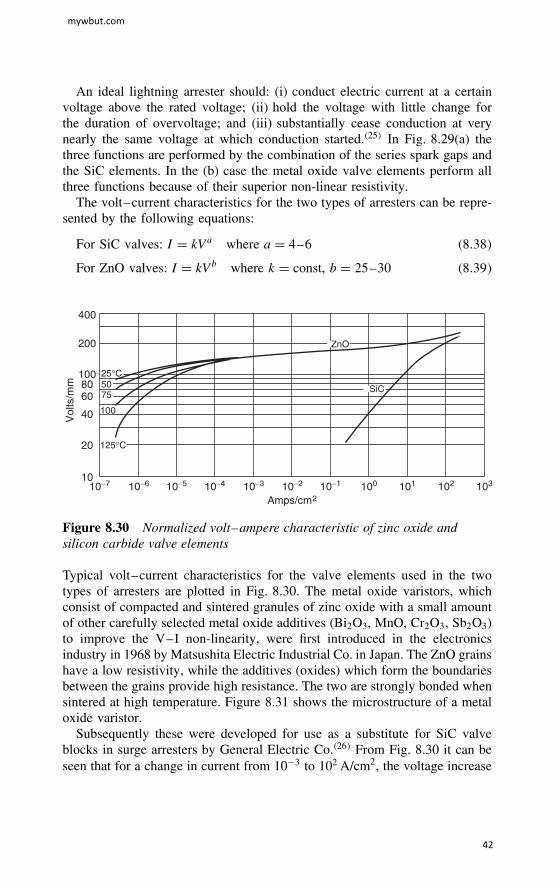
An ideal lightning arrester should: (i) conduct electric current at a certainvoltage above the rated voltage; (ii) hold the voltage with little change forthe duration of overvoltage; and (iii) substantially cease conduction at verynearly the same voltage at which conduction started.�25� In Fig. 8.29(a) thethree functions are performed by the combination of the series spark gaps andthe SiC elements. In the (b) case the metal oxide valve elements perform allthree functions because of their superior non-linear resistivity.

The volt–current characteristics for the two types of arresters can be repre-sented by the following equations:

For SiC valves: I D kVa where a D 4–6 �8.38�

For ZnO valves: I D kVb where k D const, b D 25–30 �8.39�

400

200

10080

1010−7 10−6 10−5 10−4 10−3 10−2 10−1 100 101 102 103

20

40

60

Vol

ts/m

m

Amps/cm2

25°C

125°C

ZnO

SiC5075

100

Figure 8.30 Normalized volt–ampere characteristic of zinc oxide andsilicon carbide valve elements

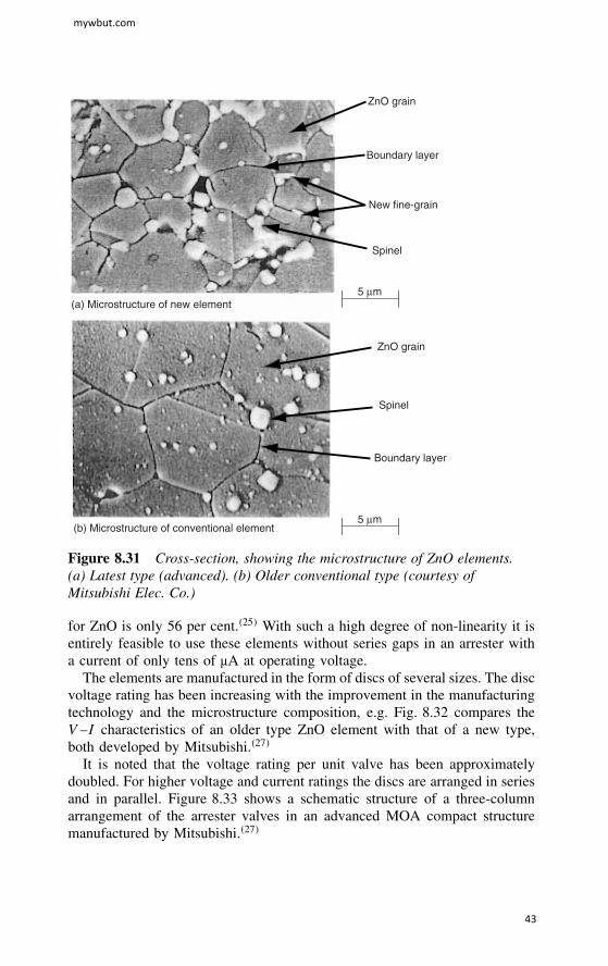
Typical volt–current characteristics for the valve elements used in the twotypes of arresters are plotted in Fig. 8.30. The metal oxide varistors, whichconsist of compacted and sintered granules of zinc oxide with a small amountof other carefully selected metal oxide additives (Bi2O3, MnO, Cr2O3, Sb2O3)to improve the V–I non-linearity, were first introduced in the electronicsindustry in 1968 by Matsushita Electric Industrial Co. in Japan. The ZnO grainshave a low resistivity, while the additives (oxides) which form the boundariesbetween the grains provide high resistance. The two are strongly bonded whensintered at high temperature. Figure 8.31 shows the microstructure of a metaloxide varistor.

Subsequently these were developed for use as a substitute for SiC valveblocks in surge arresters by General Electric Co.�26� From Fig. 8.30 it can beseen that for a change in current from 10�3 to 102 A/cm2, the voltage increase

mywbut.com

42

ZnO grain

Boundary layer

New fine-grain

(b) Microstructure of conventional element

(a) Microstructure of new element

ZnO grain

Boundary layer

Spinel

Spinel

5 µm

5 µm

Figure 8.31 Cross-section, showing the microstructure of ZnO elements.(a) Latest type (advanced). (b) Older conventional type (courtesy ofMitsubishi Elec. Co.)

for ZnO is only 56 per cent.�25� With such a high degree of non-linearity it isentirely feasible to use these elements without series gaps in an arrester witha current of only tens of µA at operating voltage.

The elements are manufactured in the form of discs of several sizes. The discvoltage rating has been increasing with the improvement in the manufacturingtechnology and the microstructure composition, e.g. Fig. 8.32 compares theV–I characteristics of an older type ZnO element with that of a new type,both developed by Mitsubishi.�27�

It is noted that the voltage rating per unit valve has been approximatelydoubled. For higher voltage and current ratings the discs are arranged in seriesand in parallel. Figure 8.33 shows a schematic structure of a three-columnarrangement of the arrester valves in an advanced MOA compact structuremanufactured by Mitsubishi.�27�

mywbut.com

43

Current density (A/cm2)

Conventional

Varistor voltage

Vol

tage

(p.

u.)

10−6 10−5 10−4 10−3 10−2 10−1 101 102 1031000.5

1

2

3

4

X

New

Figure 8.32 Comparison of volt–current characteristics of (a) advancedMOA with (b) that of an older type MOA (courtesy of Mitsubishi Co.)

Insulator

Conductor

ZnO elements

Figure 8.33 Schematic structure of a three column series arrangement ofelements in advanced MOAs

mywbut.com

44

In Fig. 8.34 is shown part of an assembled advanced 500 kV MOA. Thepercentages indicate the reduction in size by replacing the older type MOA withthe advanced MOA elements whose V–I characteristics are shown in Fig. 8.32.

AdvancedMOA

Insulatingspacer

Shield

ZnOelements

60%

92%

ConventionalMOA

500 kV

Figure 8.34 Part of an assembled 500 kV MOA Arrester. (courtesy ofMitsubishi Co.)

In this construction the individual surge arresters are interconnectedby means of corona-free stress distributors. The modular design and thelightweight construction allow easy on-site erection and in the event of anyunits failing the individual unit may be readily replaced.

The advantages of the polymeric-housed arresters over their porcelain-housed equivalents are several and include:

ž No risk to personnel or adjacent equipment during fault current operation.ž Simple light modular assembly – no need for lifting equipment.

mywbut.com

45

ž Simple installation.ž High-strength construction eliminates accidental damage during transport.ž The use of EPDM and/or silicon rubber reduces pollution flashover

problems.

Thus the introduction of ZnO arresters and their general acceptance byutilities since late 1980s, and in 1990s in protecting high voltage substations,has greatly reduced power systems protection problems.

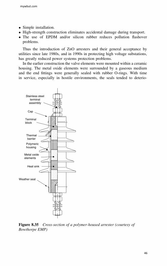
In the earlier construction the valve elements were mounted within a ceramichousing. The metal oxide elements were surrounded by a gaseous mediumand the end fittings were generally sealed with rubber O-rings. With timein service, especially in hostile environments, the seals tended to deterio-

Terminalblock

Thermalbarrier

Polymerichousing

Metal oxideelements

Heat sink

Weather seal

Cap

Stainless steelterminal

assembly

Figure 8.35 Cross-section of a polymer-housed arrester (courtesy ofBowthorpe EMP)

mywbut.com

46

rate allowing the ingress of moisture. In the 1980s polymeric-housed surgearresters were developed. Bowthorpe EMP (UK)�28� manufactures a completerange of polymeric-housed arresters extending from distribution to heavy dutystation arresters for voltages up to 400 kV. In their design the surface of themetal oxide elements column is bonded homogeneously with glass fibre rein-forced resin. This construction is void free, gives the unit a high mechanicalstrength, and provides a uniform dielectric at the surface of the metal oxidecolumn. The housing material is a polymer (EPDM)–Ethylene propylene dienemonomer–which is a hydrocarbon rubber, resistant to tracking and is partic-ularly suitable for application in regions where pollution causes a problem.A cross-section detailing the major features of a polymeric-housed arrester isgiven in Fig. 8.35.

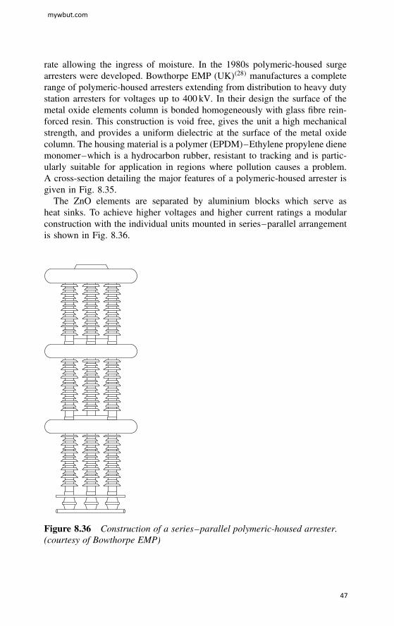
The ZnO elements are separated by aluminium blocks which serve asheat sinks. To achieve higher voltages and higher current ratings a modularconstruction with the individual units mounted in series–parallel arrangementis shown in Fig. 8.36.

Figure 8.36 Construction of a series–parallel polymeric-housed arrester.(courtesy of Bowthorpe EMP)

mywbut.com

47