chapter 8 general algebraic modeling system (gams)bussieck/gamsmodlang.pdf · chapter 8 general...
TRANSCRIPT
Chapter 8
GENERAL ALGEBRAIC MODELING SYSTEM(GAMS)
Michael R. Bussieck & Alex MeerausGAMS Development Corporation
Washington D.C., U.S.A.
{MBussieck,AMeeraus}@gams.com
Abstract In this chapter we will categorize the development of mathematical programmingtools into three major phases and will define three major categories of modelsand their use. This classification will be used to describe some of the featuresfound inGAMS to support different application environments. Selected languagefeatures, and examples of external functions and privacy and security issues arediscussed and separate annexes. Finally, we will list the inputs to a problem thathas been provided to all the authors by the editor of this volume.
Introduction
Today, algebraic modeling languages are widely accepted as the best wayto represent and solve mathematical programming problems. Their main dis-tinguishing features are the use of relational algebra and the ability to providepartial derivatives on multidimensional, very large and sparse structures. Inthis chapter we will describe some of the origins ofGAMS and provide back-ground information that shaped early design decisions. Initial Research andDevelopment ofGAMSwas funded by the International Bank for Reconstructionand Development, usually referred to as The World Bank, through the Bank’sResearch Committee (RPO 671-58, RPO 673-06) and carried out at the Devel-opment Research Center in Washington DC. Since 1987, R&D has been fundedby GAMS Development Corporation.
The system was developed in close cooperation of mathematical economistswho were and still are an important group ofGAMS users. The synergy betweeneconomics, computer science and operations research was the most importantsuccess factor in the development of the system. Mathematical Programming
137

138 MODELING LANGUAGES IN MATHEMATICAL OPTIMIZATION
and economics theory are closely intertwined. The Nobel Prize in Economicsawarded to Leonid Kantorovich and Tjalling Koopmans in 1975 for their “con-tribution to the theory of optimal allocation of resources” was really a prizein mathematical programming. Other Nobel laureates like Kenneth Arrow in1972, Wassily Leontief in 1973, and Harry Markowitz in 1990 are well knownnames in math programming. Another early example of this synergy is the useof LP in refining operations, which was started by Alan Manne, an economist,with his book onScheduling of Petroleum Refinery Operationsin 1956 [148].
The origins of linear programming algorithms all go back to George Dantzig’searly work in the 1940s and 1950s [44, 45]. Computing technology and algo-rithmic theory had developed at a rapid pace. Thirty years later, we could solveproblems of practical size and complexity that allowed us to test of the eco-nomic theory on real life problems. The research agenda at the World Bank inthe 1970s and 1980s created the perfect environment to bring different disci-plines together to apply mathematical programming to research and operationalquestions in Economic Development.
8.1 Background and Motivation
From the very beginning, the driving force behind the development of theGeneral Algebraic Modeling System (GAMS) [26] has been the users of mathe-matical programming who believed in optimization as a the powerful and elegantframework for solving real life problems in the sciences and engineering. Atthe same time, these users were frustrated with the high cost, skill requirements,and overall low reliability of applying optimization tools. Most of our initia-tives and support for new development came from the worlds of economics,finance, and chemical engineering. These disciplines find it natural to view andunderstand the world and its behavior as a mathematical program.
GAMS’s impetus for development arose out of the frustrating experiences of alarge economic modeling group at the World Bank. In hindsight, one may callit a historical accident that in the 1970s mathematical economists and statisti-cians were assembled to address problems of development. They used the besttechniques available at the time to solve multisectoral economy-wide modelsand large simulation and optimization models in agriculture, steel, fertilizer,power, water use, and other sectors. Although the group produced impres-sive research, initial successes were difficult to reproduce outside their wellfunctioning research environment. The existing techniques to construct, ma-nipulate, and solve such models required several manual, time-consuming, anderror-prone translations into the different, problem-specific representations re-quired by each solution method. During seminar presentations, modelers hadto defend the existing versions of their models, sometimes quite irrationally, be-cause the time and money needed to make proposed changes were prohibitive.

General Algebraic Modeling System (GAMS) 139
Their models just could not be moved to other environments, because specialprogramming knowledge was needed, and data formats and solution methodswere not portable.
The idea of an algebraic approach to represent, manipulate, and solve large-scale mathematical models fused old and new paradigms into a consistent andcomputationally tractable system. Using matrix generators (see appendixGAMSversus Fortran Matrix Generators) for linear programs taught us the importanceof naming rows and columns in a consistent manner. The connection to theemergingrelational datamodel became evident. Painful experience using tra-ditional programming languages to manage those name spaces naturally leadone to think in terms of sets and tuples, and this led to the relational data model.Combining multidimensional algebraic notation with the relational data modelwas the obvious answer. Compiler writing techniques were by now widespread,and languages likeGAMS could be implemented relatively quickly. However,translating this rigorous mathematical representation into the algorithm specificformat required the computation of partial derivatives on very large systems. Inthe 1970s, TRW developed a system called PROSE [203] that took the ideas ofchemical engineers to computepoint derivativesthat were exact derivatives at agiven point, and to embed them in a consistent, fortran-style calculus modelinglanguage. The resulting system allowed the user to use automatically generatedexact first and second order derivatives. This was a pioneering system and animportant demonstration of a concept. However, in our opinion PROSE had anumber of shortcomings: it could not handle large systems, problem represen-tation was tied to an array-type data structure that required address calculations,and the system did not provide access to state-of-the art solution methods. Fromlinear programming, we learned that exploitation of sparsity was the key to solvelarge problems. Thus, the final piece of the puzzle was the use ofsparse datastructures.
With all pieces in place, all we had to do was adopt the techniques to fit intoone consistent framework and make it work for large problems.
8.2 Design Goals and Changing Focus
The original and still valid goal is to improve the model builder’s productivity,reduce costs, and improve reliability and overall credibility of the modelingprocess. To achieve this, we established the following key principles to guidetheGAMS development:
The problem representation is independent of the solution method.
The data representation follows the relational data model.
The problem and data representations are independent of computing plat-forms.

140 MODELING LANGUAGES IN MATHEMATICAL OPTIMIZATION
The problem and data representations are independent of user interfaces.
Optimization methods will fail, and systems have to be designed to befail-safe.
Another way to express these principles is to think in terms of layers of rep-resentations and capabilities that have clearly defined interfaces and functions.The oldest and most basic layer is thesolver layeror implementation of a spe-cific algorithm. Above the solver is the model layer, expressed in an algebraicmodeling language. Themodeling layertranslates the mathematical represen-tation into a computational structure required by a specific solution method andprovides various services such as function and derivative evaluations and errorrecovery. Above the modeling layer is theapplication or domain layer, whichis highly context sensitive and has knowledge about the problem to be solvedand the kind of user interacting with the system.
It is instructive to put the development of modeling systems into some historicperspective and see how the focus and technical constraints have changed in thelast 30 years. We can observe three major phases that shift the emphasis fromcomputational issues to modeling issues and finally the application or the realproblems. Each phase defined one of the main system layers discussed above.The dominant constraints in the first phase were thecomputational limitsof ouralgorithms. Problem representation had to abide by algorithmic convenience,centralized expert groups managed large, expensive and long lasting projectsand end users were effectively left out. The second phase has themodelin focus.This volume is about languages and systems supporting this stage. Applicationsare limited by modeling skill, project groups are much smaller and decentralized,the computational cost are low and the users are involved in the design ofthe application. Applications are designed to be independent of computingplatforms and frequently operate in a client-server environment.
We believe that we are entering a third phase which has theapplicationasits focus and the optimization model is just one of many analytic tools thathelp making better decisions. The users are often completely unaware of anyoptimization model or use a mental model that is different from the actual modelto solved by optimization techniques. User interfaces are build with off-the-shelf components and frequently change to adjust to evolving environments andnew computing technologies. As with databases, modeling components have amuch longer life than user interfaces. We have observed cases where the modelhas remained basically unchanged over many years, whereas the computingenvironments and user interfaces have changed several times. The solvers usedto solve the models have changed, the computing platforms have changed, theuser interfaces have changed and the overall performance of the model haschanged without any change in the model representation.
General Algebraic Modeling System (GAMS) 141
8.3 A User’s View of Modeling Languages
Today’s modeling systems have achieved an interface between the solver andthe model world. They also attempt to provide solutions for interfacing modelsand applications. These attempts focus mainly on data exchange capabilities,source code generation, and access to model object libraries. None of these sug-gested solutions has yet been widely accepted. This area will remain very activefor the next decade, and may ultimately decide which optimization technologybecomes the most widely used in tomorrow’s applications. In this section wedescribe requirements for a modeling system for different classes of models andusers. We segment the world of models into three categories:
academic research models,
domain expert models, and
black box models.
We also illustrate various concepts, currently implemented in theGAMS system,that support the modeling process from each user’s perspective. Each sectionstarts by describing the typical environment and user supported by some actualexamples. Furthermore, we discuss how particularGAMS features, that are notnecessarily found in other systems, might help these users.
8.3.1 Academic Research Models
Academic research models implement mathematical programming problemsoften found in academic publications. The model source consists almost ex-clusively of highly complex algebra that defines the variables and equations.Frequently, these kinds of models, that are benchmarked using a given set ofpublicly available test instances, support statements made in research papers.An impressive library of test problems from Operations Research can be foundin the OR Library [9]. In addition to obvious selection criterion such as per-sonal taste for syntax and the development environment, the most importantcriteria for selecting a modeling system for these kind of models are the avail-ability of the user’s platform of choice and the availability of the model typeand appropriate solver.
GAMS offers mixed integer linear and nonlinear programming model types,mixed complementarity problem (MCP) type, and mathematical programs withequilibrium constraints (MPEC). MCP and MPEC play an important role ineconomic modeling. In addition,GAMS can represent multi-level stochastic opti-mization problems and models with cone constraints. Furthermore, applicationlanguages like MPSGE for general equilibrium models and LOGMIP for dis-junctive programming provide access to optimization techniques to researchersoutside our narrow field of mathematical programming. To seamlessly support

142 MODELING LANGUAGES IN MATHEMATICAL OPTIMIZATION
new model types or solvers, theGAMS language offers sufficient flexibility torepresent new ideas within the current syntax (although certain constructs maylook somewhat awkward). The idea is to first understand each new concept’smodel, algorithms, and most important application areas, before adding syntaxfrom that concept to an increasingly cluttered language.
One ofGAMS’ early design criteria was to be both platform and solver inde-pendent.GAMS users immediately benefit from hardware and operating systemimprovements, and improvements on the solver side. Throughout its evolution,theGAMS system has seen the rise and fall of quite a few platforms and mathe-matical programming solvers. We anticipate a similar pattern in the future. Thesolver suite of the actualGAMS system includes about 20 supported solvers anda handful of contributed plug-and-play solvers. Each supportedGAMS solvercomplies to a strictly defined solver interface, making the seamless exchange ofsolvers possible for aGAMSmodeler. Common solver attributes (e.g., maximumresource time) can be set through generalGAMS options, and solver-specific op-tions can be set through option files. Linking a solver toGAMSmeans complyingwith this strict interface, which can be a challenging task1. There are easier waysto connect to a modeling system, especially for research codes. For example,theAMPL (see Chapter 7) input/output library is geared towards convenience forthe algorithm provider. We find many research codes hooked up toAMPL (e.g.,most NEOS solvers have anAMPL interface). Making these codes available forGAMS models would allow researchers to benchmark theirGAMS models againsta larger set of solvers, without reformulating their model in different modelinglanguages. Rather than compromising the strictGAMS solver interface, theGAMSsystem comes with a translationsolvercalled CONVERT [29].
Modeling languages have a rich syntax that is usually based on sets andindexed variables, equations, and parameters. This syntax, the correspondingstructure in the model, and the data is very useful to the model developer.However, this structure is not used by the solvers. Most solvers see the worldas consisting of a list of variables (X1 toXn), a list of equations or constraints(E1 to Em), and the relationship between these variables and equations, asrepresented in some form. It is therefore acceptable for a translator to removethe structure, as long as the model as seen by the solver remains unchanged.
The translation solver CONVERT transforms models into a very simple inter-nal scalar format. This internal format can then be written out in many differentformats.
With GAMS as output format, the scalar model consists of
1The title of the corresponding documentation says it all:Linking your Solver toGAMS. The Complete Notes.Don’t Panic!!

General Algebraic Modeling System (GAMS) 143
Set I Products /P1*P2/J Cutting Patterns /C1*C2/;
Parameter c(J) cost of raw material /C1 1, C2 1/cc(J) cost of change-over of knives /C1 0.1, C2 0.2/b(I) width of product roll-type I /P1 460, P2 570/nord(I) number of orders of product type I /P1 8, P2 7/Bmax width of raw paper roll /1900/Delta tolerance for width / 200/Nmax max number of products in cut / 5/bigM max number of repeats of any pattern / 15/;
Variable y(J) cutting patternm(J) number of repeats of pattern jn(I,J) number of products I produced in cut Jobj objective variable;
Binary Variable y; Integer Variable m, n;
Equation defobj, max_width(J), min_width(J), max_n_sum(J),min_order(I), cut_exist(J), no_cut(J);
defobj.. sum(j, c[j]*m[j] + cc[j]*y[j]) =e= obj;max_width(j).. sum(i, b[i]*n[i,j]) =l= Bmax;min_width(j).. sum(i, b[i]*n[i,j]) + Delta =g= Bmax;max_n_sum(j).. sum(i, n[i,j]) =l= Nmax;min_order(i).. sum(j, m[j]*n[i,j]) =g= nord[i];cut_exist(j).. y[j] =l= m[j];no_cut(j).. m[j] =l= bigM*y[j];
m.up[j] = bigM; n.up[i,j] = nmax;
model trimloss /all/;solve trimloss minimize obj using minlp;
Figure 8.3.1. The orginialGAMS model for trim loss optimization
declarations of the variables, with extra declarations for the subsets ofpositive, integer, or binary variables;
declarations of the equations;
the symbolic form of these equations; and
assignment statements for non default bounds and initial values.
All operations involving sets are unrolled, and all expressions involving pa-rameters are evaluated and replaced by their numerical values. Since there areno sets or indexed parameters in the scalar models, most of the differences be-tween modeling systems have disappeared. Therefore, theGAMS format can betransformed easily into the format of another language. InAMPL, for example,
144 MODELING LANGUAGES IN MATHEMATICAL OPTIMIZATION
* MINLP written by GAMS Convert
Variables b1,b2,i3,i4,i5,i6,i7,i8,x9;
Binary Variables b1,b2;Integer Variables i3,i4,i5,i6,i7,i8;
Equations e1,e2,e3,e4,e5,e6,e7,e8,e9,e10,e11,e12,e13;
e1.. 0.1*b1 + 0.2*b2 + i3 + i4 - x9 =E= 0;e2.. 460*i5 + 570*i7 =L= 1900;e3.. 460*i6 + 570*i8 =L= 1900;e4.. 460*i5 + 570*i7 =G= 1700;e5.. 460*i6 + 570*i8 =G= 1700;e6.. i5 + i7 =L= 5;e7.. i6 + i8 =L= 5;e8.. i3*i5 + i4*i6 =G= 8;e9.. i3*i7 + i4*i8 =G= 7;e10.. b1 - i3 =L= 0;e11.. b2 - i4 =L= 0;e12.. - 15*b1 + i3 =L= 0;e13.. - 15*b2 + i4 =L= 0;
* set non default boundsi3.up = 15; i4.up = 15; i5.up = 5;i6.up = 5; i7.up = 5; i8.up = 5;
Model m / all /;Solve m using MINLP minimizing x9;
# MINLP written by GAMS Convert
var b1 binary;var b2 binary;var i3 integer >= 0, <= 15;var i4 integer >= 0, <= 15;var i5 integer >= 0, <= 5;var i6 integer >= 0, <= 5;var i7 integer >= 0, <= 5;var i8 integer >= 0, <= 5;
minimize obj: 0.1*b1 + 0.2*b2 + i3 + i4;subject to
e2: 460*i5 + 570*i7 <= 1900;e3: 460*i6 + 570*i8 <= 1900;e4: 460*i5 + 570*i7 >= 1700;e5: 460*i6 + 570*i8 >= 1700;e6: i5 + i7 <= 5;e7: i6 + i8 <= 5;e8: i3*i5 + i4*i6 >= 8;e9: i3*i7 + i4*i8 >= 7;e10: b1 - i3 <= 0;e11: b2 - i4 <= 0;e12: - 15*b1 + i3 <= 0;e13: - 15*b2 + i4 <= 0;
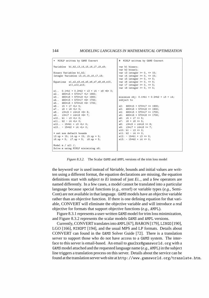
Figure 8.3.2. The ScalarGAMS andAMPL versions of the trim loss model
the keywordvar is used instead ofVariable, bounds and initial values are writ-ten using a different format, the equation declarations are missing, the equationdefinitions start withsubject to Eiinstead of justEi.., and a few operators arenamed differently. In a few cases, a model cannot be translated into a particularlanguage because special functions (e.g., errorf) or variable types (e.g., Semi-Cont) are not available in that language.GAMSmodels have an objective variablerather than an objective function. If there is one defining equation for that vari-able, CONVERT will eliminate the objective variable and will introduce a realobjective for formats that support objective functions (e.g., AMPL).
Figure 8.3.1 represents a user-writtenGAMSmodel for trim loss minimization,and Figure 8.3.2 represents the scalar modelsGAMS andAMPL versions.
Currently, CONVERT translates intoAMPL [67], BARON [179],LINGO [190],LGO [166],MINOPT [194], and the usual MPS and LP formats. Details aboutCONVERT can found in theGAMS Solver Guide [72]. There is a translationserver to support those who do not have access to aGAMS system. The inter-face to this server is email-based. An email [email protected] with aGAMSmodel attached and the requested language name (e.g.,AMPL) in the subjectline triggers a translation process on this server. Details about the service can befound at the translation server web site athttp://www.gamsworld.org/translate.htm.
General Algebraic Modeling System (GAMS) 145
8.3.2 Domain Expert Models
Domain expert models are often used as tools for problem analysis. To be auseful tool and to be able to support a user over a decade or more, thesemodelsneed to be highly flexible. During its lifetime, a domain expert model growsand changes with every new project the domain expert takes on. The meaningof the termmodelalso changes dramatically, from a collection of equations andvariables to a compilation of sophisticated modules that prepare data, find aso-lution to a problem, and provide reporting capabilities. Mathematical programsare often included in the data preparation model (e.g., calibration of data), andin the solution module, intertwined with other algorithmically steps. The partthat represents mathematical programs (i.e., equations and variables) does not,however, often exceed 10% of the overall code (the major part ofGAMS sourcecode is dedicated to data calculations and reporting).
The domain experts who use these models have entirely different needs thando the users of academic research models. A perfect example of such a domainexpert user is the consulting firm Hill & Associates in Annapolis, Maryland,U.S.A. This firm specializes in providing sound advise and management servicesto the coal and electricity markets, based on supply, demand, and transportationdata gathered over the past two decades. The models used in theirElectricGeneration, Coal and Emission Forecasting Systeminclude several extremelychallenging linear and mixed-integer linear problems with millions of variablesand hundreds of thousands of constraints. Since the requirements for this sys-tem change with nearly every project, the computing environment needs to behighly modular and to grow over time. Since the final product of a consultant issome written report, the models need to communicate with many data systems,including databases of different vintage and presentation systems such as Map-Info. Highly skilled experts, primarily economists and engineers, operate thesemodels, and have deep insight into them and their application. Failures are thenorm in such a constantly changing system, and handling failures is part of theroutine operation.
TheGAMS system fits nicely into such a diverse environment because it in-terfaces well with other systems. Data exchange with other modules is ac-complished through theGAMS Data eXchange (GDX) facilities, a collectionof ready-made programs that communicate with standard applications and anapplication programming interface (API) for custom-made data exchange. Fur-thermore, theGAMS execution system seamlessly integrates with external pro-cedures, including a model’s equations (seeExternal Functions inGAMSin theappendix). This capability makes it very easy to integrate aGAMS model into alarge application (a collection of such application systems was presented on theback cover of OR/MS Today issues from 1999 to 2001).
146 MODELING LANGUAGES IN MATHEMATICAL OPTIMIZATION
The GDX facilities complement theGAMS system’s ASCII-based input andoutput. In addition to improving input/output time for bulk data movements, thedata coming through the GDX interface is guaranteed to be syntactically cor-rect. This inconspicuous feature, combined with a well-defined data contract(a mapping between the name-space in theGAMS model and the name-space inthe external data source), allows the user to segment responsibility for interfac-ing the model with other systems. This segmentation is often reflected in theoptimization project structures found at larger companies, where model ana-lysts and developers ensure the correctness of the model, and the IT departmentguarantees the accurate transfer of data. Smooth operation is guaranteed if bothgroups adhere the data contract. If an error occurs, it can easily be traced to itssource, to ensure that repair responsibility is properly assigned.
In modeling systems where the data exchange is part of the language, thedata contract must reside inside the model.GAMS and GDX allow this contractto reside anywhere. This is especially helpful with spreadsheets and other caseswhere it is advantageous to place the data contract inside the data source.2 Inother applications where model and database are components of a larger system,it may be necessary to place the data contract between the model and the databaseinside the driving application.
The GDX interface can also be used to capture data in a database type file,called the GDX file. This file contains parameters, sets, and even scalar-likelevel and marginal values of variables and equations. All input data required fora model run can be represented in this platform-independent file (even across bigand little endian computers). This ensures capture of the instance of a modelfailure. The problem can then be analyzed off-line together with the modelsource, and does not require otherwise vital connections with the rest of theapplication system.
Capturing the model source can frequently be as complex a process as ob-taining the data itself, since the source can reside in different files located indifferent directories. Therefore,GAMS provides a source dumping mechanism(dumpopt) to collect all model sources in one file.
Independent of the original data source, the GDX file represents a highlystructured database. Supplemented by a collection of GDX tools, the GDXfacilities provide an environment that makes it easy to analyze both the datathat goes into a model and the results that come out of each model run. Forexample, the toolgdxdiffcompares two GDX files and reports differences sim-ilar to the UNIXdiff text utility. To compare numeric data settings, an absolutetolerance allows the user to filter the differences. The utilitiesgdxmergeandgdxsplitcombine structurally identical GDX files and add a scenario index to
2The GDX utility gdxxrw, which exchanges data with MS-Excel, supports this with itsparam=indexoption.For details see http://www.gams.com/dd/docs/gams/gdxutils.pdf.
General Algebraic Modeling System (GAMS) 147
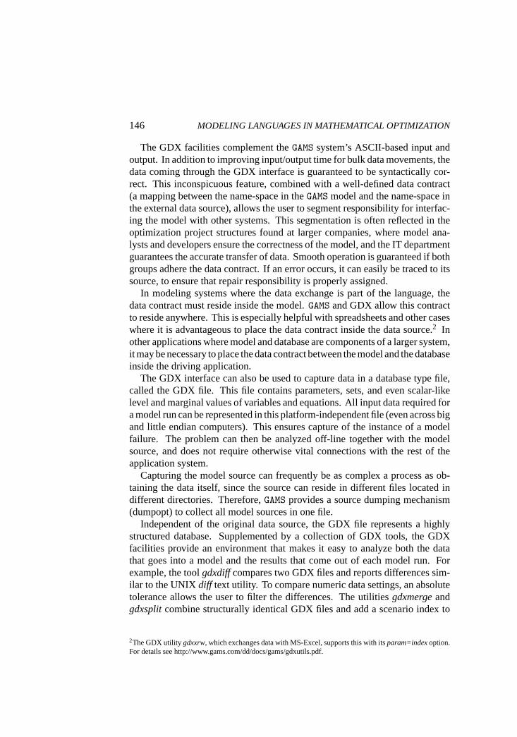
Figure 8.3.3. Scenario Management Tool:VEDA
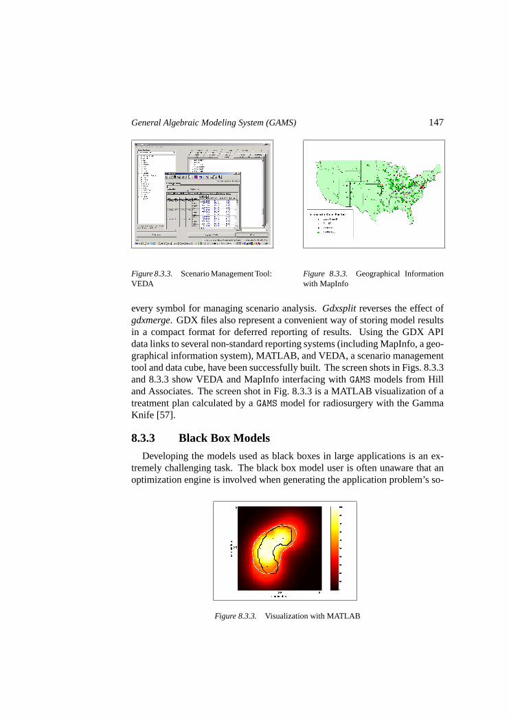
Figure 8.3.3. Geographical Informationwith MapInfo
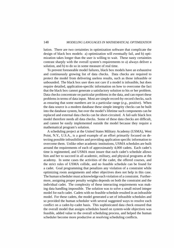
every symbol for managing scenario analysis.Gdxsplitreverses the effect ofgdxmerge. GDX files also represent a convenient way of storing model resultsin a compact format for deferred reporting of results. Using the GDX APIdata links to several non-standard reporting systems (including MapInfo, a geo-graphical information system), MATLAB, and VEDA, a scenario managementtool and data cube, have been successfully built. The screen shots in Figs. 8.3.3and 8.3.3 show VEDA and MapInfo interfacing withGAMS models from Hilland Associates. The screen shot in Fig. 8.3.3 is a MATLAB visualization of atreatment plan calculated by aGAMS model for radiosurgery with the GammaKnife [57].
8.3.3 Black Box Models
Developing the models used as black boxes in large applications is an ex-tremely challenging task. The black box model user is often unaware that anoptimization engine is involved when generating the application problem’s so-
Figure 8.3.3. Visualization with MATLAB
148 MODELING LANGUAGES IN MATHEMATICAL OPTIMIZATION
lution. There are two certainties in optimization software that complicate thedesign of black box models: a) optimization will eventually fail, and b) opti-mization takes longer than the user is willing to wait. These nasty certaintiescontrast sharply with the overall system’s requirements to a) always deliver asolution, and b) to do so in some measure of real time.
To prevent foreseeable model failures, black box models have an exhaustiveand continuously growing list of data checks. Data checks are required toprotect the model from delivering useless results, such as those infeasible orunbounded. The black box user does not care if a model is infeasible, but doesrequire detailed, application-specific information on how to overcome the factthat the black box cannot generate a satisfactory solution to his or her problem.Data checks concentrate on particular problems in the data, and can report theseproblems in terms of data input. Most are simple record-by-record checks, suchas ensuring that some numbers are in a particular range (e.g., positive). Whenthe data source is a modern database these simple integrity checks can be builtinto the database system, but over the model’s lifetime such components can bereplaced and external data checks can be short-circuited. A fail-safe black boxmodel therefore needs all data checks. Some of these data checks are difficult,and cannot be easily implemented outside the model because they require amathematical program’s solution.
A scheduling project at the United States Military Academy (USMA), WestPoint, N.Y., U.S.A., is a good example of an effort primarily focused on de-tecting possible infeasibilities and providing application specific information toovercome them. Unlike other academic institutions, USMA schedules are builtaround the requirements of each of approximately 4,000 cadets. Each cadet’stime is regimented, and USMA must insure that each cadet’s schedule allowshim and her to succeed in all academic, military, and physical programs at theacademy. In some cases the activities of the cadet, the offered courses, andthe strict rules of USMA collide, and no feasible schedule can be found fora cadet. Goal programming that penalizes any violation of a constraint whileoptimizing room assignments and other objectives does not help in this case.The human scheduler must acknowledge each violation of a constraint. Further-more, assigning proper penalty weights depends on both the constraint and theindividual cadet. The complexity of these interacting requirements was mak-ing data handling impossible. The solution was to solve a small mixed integermodel for each cadet. Cadets with no feasible schedule resulted in an infeasiblemodel. For these cadets, the model generated a set of infeasible schedules andso provided the human scheduler with several suggested ways to resolve eachconflict on a cadet-by-cadet basis. This sophisticated data check ensured thatthe overall model that assigns schedules based on system-wide objectives wasfeasible, added value to the overall scheduling process, and helped the humanscheduler become more productive at resolving scheduling conflicts.
General Algebraic Modeling System (GAMS) 149
A black box optimization model is often a central but small part of a largeapplication system. The most prominent requirement is reliability in the modeland the underlying modeling system. Data checks are one way to make themodel reliable. Another way is to anticipate the solution module’s failure andhave a back-up solution ready. TheGAMS execution system’s flow control state-ments allow the user to build simple heuristics for most problems. The user getsa back-up solution, and the model can automatically capture the problematicinstance (e.g., in a GDX file) for off-line analysis by the model developer. Theoverall model cannot collapse just because a solver crashed with some hard ex-ception error. The modeling system must be able to recover from such failures,and also needs watchdog capabilities to keep solver resources (e.g., time andmemory) in check. TheGAMS system can run the solver completely detachedfrom the overall model processing. This protects the model from unintentionalinterference from the solver or other external processes.
The world of platform independent development with Java and advances ininternet-ready application shed new light on the importance of platform inde-pendence for modeling systems. For example, an optimization application’sdevelopment might start on Windows PCs, undergo testing on Solaris work-stations, deploy an optimization module on an HP workstation, and move to a64-bit Linux PC after five years.
8.4 Summary and Conclusion
In this chapter we provided some background information to support andexplain some of the early design decisions, which we believe are still valid todayand guide us into the future. As a language and modeling system designers it isimportant to keep the focus on the existing and future user community. Mundaneconcepts as backward compatibility are an essential element in protecting theinvestments of our users. They demand that models built 10 years ago canbe operated today without any change and at the same time are able to takeadvantage of the latest computer architecture and technology as well allow theuse of any state-of-the-art solvers. The same holds for an unknown futuremodeling environments. The users of our systems are entitled to expect thattheir models will operate in 10 years from now with out any change. Theincorporation of new technologies and theoretical advances will have to bedone in a way to protect existing investments.
Finally we would like to recognize the contribution of the editor of this vol-ume, Dr. Josef Kallrath, to bring together a group of highly individualistic andsometimes very competitive developers at the 2003 meeting in Bad Honnef andmanage to make them contribute the chapters in a timely fashion. Congratula-tions.

150 MODELING LANGUAGES IN MATHEMATICAL OPTIMIZATION
Appendix
A Selected Language FeaturesThe modeling systems described in this volume are closely related to each other and share
many important design principles and in many cases look very similar. The following is asomewhat arbitrary list of features that are not shared by other systems:
Model Types. A model is a collection of symbolic equations which can be used to solvea specific model type with a statement likesolve mymodel using NLP minimizing myobjective.GAMS requires the user to specify the general model type. This allows the system to verify that asuitable solver is available and that the symbolic algebra fits into the general problem class. Sincea nonlinear mixed-integer problem is magnitudes more difficult to solve than a linear program,GAMS requires the user to be aware of the kind of model he or she wants to build and solve. Thesecond feature is thatGAMS does not have an objective function and uses instead a simple variableto express the maximand. This allows any variable or indirectly any constraint to serve as anobjective at the point of model instantiation.
Attached Comments.Comment and explanatory texts are permanently attached to all symbolsand data elements. Descriptive information will never be lost and can automatically be retrievedwhen producing reports or display intermediate results. This encourages good modeling practiceand provides automatic documentation.
Domain Checking.Index positions of all data types aredomain checked. This is very similarto the concept of referential integrity in data base systems and will guarantee that we will neverattempt to reference an index position with an incorrect elopement, set or subset that does notbelong there. For example, a variable declared to have the index context of the sets (I,J) can onlybe indexed by thedomain setsI and J, their subsets or elements belonging to them. All commonerrors of inadvertently transposing index references like (J,I) will be flagged as errors.
No Dummy Index. Index references do not usedummy indices. In most cases, the useof dummy indicesmakes the algebra more difficult to read and leads to a loss of context. Forexample, a matrix multiplication is simply written asc(i,j) = sum(k, a(i,k)*b(j,k)). A good namingconvention then leads to a very compact and direct representation. A consequence of this choiceis need for ’aliases’ to allow driving more than one index with the same set.
Relaxed Punctuation.A certain amount of context sensitivity andrelaxedpunctuation isallowed. Non-programmers become very impatient if every string has to be quoted, or a missingcomma at the end of a line in some list causes a compilation error. Another example is a missingstatement separator ’;’ not causing any ambiguity will not cause an error.
Common Syntax for Declarative and Procedural Components.The syntax for data trans-formations and symbolic equation definitions are alike and treated internally in the same way.Symbolic equation, model and data definitions are declarative, all other statements are proce-dural. As problems become more complex, the procedural aspects of the system become moreimportant. Models of different types feed result into other models, all embedded in some complexcontrol structures.
Simple Macros.Extensive compile time source preprocessing and recursive calling ofGAMSitself allows easy tailoring of complex applications.
Computational Performance.Sparsity and parallelism are exploited to skip over “dead”indices and in most cases the order of computational burden is proportional to the number ofno default (zero) entries in its operands. For example, the computational burden ofsum((i,j),a(i,j)*x(i,j)) will be proportional to the non-zero entries in ’a’ and not the product of the cardinalityof the sets i and j.
General Algebraic Modeling System (GAMS) 151
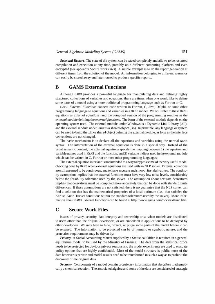
Save and Restart.The state of the system can be saved completely and allows to be restartedcompilation and execution at any time, possibly on a different computing platform and evenencrypted (see appendixSecure Work Files). A simple example is to do the report generation atdifferent times from the solution of the model. All information belonging to different scenarioscan easily be stored away and later reused to produce specific reports.
B GAMS External FunctionsAlthough GAMS provides a powerful language for manipulating data and defining highly
structured collections of variables and equations, there are times when one would like to definesome parts of a model using a more traditional programming language such as Fortran or C.
GAMSExternal Functionsconnect code written in Fortran, C, Java, Delphi, or some otherprogramming language to equations and variables in aGAMS model. We will refer to theseGAMSequations asexternal equations, and the compiled version of the programming routines as theexternal moduledefining theexternal functions. The form of the external module depends on theoperating system used. The external module under Windows is a Dynamic Link Library (.dll),and the external module under Unix is a shared object (.so). In principle, any language or systemcan be used to build the .dll or shared object defining the external module, as long as the interfaceconventions are not changed.
The basic mechanism is to declare all the equations and variables using the normalGAMSsyntax. The interpretation of the external equations is done in a special way. Instead of theusual semantic content, the external equations specify the mapping between 1) the equation andvariable names used inGAMS and the function, and 2) variable indices used in the external modulewhich can be written in C, Fortran or most other programming languages.
The external equation interface is not intended as a way to bypass some of the very useful modelchecking done byGAMSwhen external equations are used with an NLP solver. External equationsare still assumed to be continuous, and to have accurate and smooth first derivatives. The continu-ity assumption implies that the external functions must have very low noise levels, considerablybelow the feasibility tolerance used by the solver. The assumption about accurate derivativesimplies that derivatives must be computed more accurately that can be done with standard finitedifferences. If these assumptions are not satisfied, there is no guarantee that the NLP solver canfind a solution that has the mathematical properties of a local optimum (i.e., that satisfies theKarush-Kuhn-Tucker conditions within the standard tolerances used by the solver). More infor-mation aboutGAMS External Functions can be found at http://www.gams.com/docs/extfunc.htm.
C Secure Work FilesIssues of privacy, security, data integrity and ownership arise when models are distributed
to users other than the original developers, or are embedded in applications to be deployed byother developers. We may have to hide, protect, or purge some parts of the model before it canbe released. The information to be protected can be of numeric or symbolic nature, and theprotection requirements may be driven by:
Privacy. A Social Accounting Matrix supplied by a Statistical Office is required in a generalequilibrium model to be used by the Ministry of Finance. The data from the statistical officeneeds to be protected for obvious privacy reasons and the model experiments are used to evaluatepolicy options that are highly confidential. Most of the model structure is public, most of thedata however is private and model results need to be transformed in such a way as to prohibit thediscovery of the original data.
Security.Components of a model contain proprietary information that describes mathemati-cally a chemical reaction. The associated algebra and some of the data are considered of strategic

152 MODELING LANGUAGES IN MATHEMATICAL OPTIMIZATION
importance and need to be hidden completely. However, the final model will be used at differentlocations around the world.
Integrity. Data integrity safeguards are needed to assure the proper functioning of a model.Certain data and symbolic information needs to be protected from accidental changes that wouldcompromise the model’s operation.
To address these secure work file issues, access control at a symbol level and secure restartfiles have been added to theGAMS system.
Access Control. The access toGAMS symbols, including sets, variables, parameters, andequations, can be changed once with the compile time commands $purge, $hide, $protect and$expose. $Purge will remove any information associated with this symbol. $Hide will make thesymbol and all its information invisible. $Protect prevents changes to information. $Expose willrevert the symbol to its original state.
Secure Restart Files.TheGAMS licensing mechanism can be used to save a secure model ina secure work file (work files are used to save and restart the state of aGAMS program). A securework file behaves like any other work file, but is locked to a specific users license file. A privacylicense, the license file of the target users, is required to create a secure work file. The contentof a secure work file is disguised and protected against unauthorized access via theGAMS licensemechanism.
A special license is required to set the access controls and to create a corresponding se-cure work file. Reporting features have been added to allow audits and traces during genera-tion and use of secure work files. More information about secure work files can be found athttp://www.gams.com/docs/privacy.pdf
D GAMS versus Fortran Matrix GeneratorsIn the late 70’s and early 80’s, the MPS file was the universally accepted format to describe
a linear program. Those MPS files were either described using specialized Matrix Generatorlanguages, like the very successful and durableMAGEN/OMNI family of products from HaverlySystems [92], or general purpose programming languages, like Fortran and PL/I were used towrite matrix generator programs. Considerable programming experience and a large stock ofprograms had been accumulated and novel approaches like algebraic modeling languages wereviewed as irrelevant academic exercises. Computing power was still the limiting factor and theidea of replacing the MPS file with an algebraic model representation with the need to create anew instance of this model for each optimization step was considered totally impractical.
The firstGAMS implementation was done on Control Data Corporation’s (CDC) super com-puters and interfaced with the APEX [33] linear programming system which was the first highperformance system utilizing super sparse matrix technology allowing all in-core solutions. TheGAMS development team was determined to disprove the allegation of inherently poor perfor-mance of a mathematical approach. The implantation took full advantage of the CDC computingarchitecture and implemented novel dynamic data structures and just in time generation of ma-chine code was employed. The system was blazingly fast, and attracted the hoped for attentionin the traditional LP shops. The second implementation ofGAMS focused on computing platformand solver independence with the main goal to operate on IBM’s mainframes in conjunctionwith the MPSX [105] or MPSIII [124] linear programming systems, a computing environmentthat supported 90 percent of all commercial linear programming. A new product from IBM,the Optimization Subroutine Library (OSL) was used as the new performance benchmark. Theperformance target was to generate aGAMS models instance and load it into the OSL workspacein less time than it took to run the Fortran generator and read an MPS file into OSL. One of the
General Algebraic Modeling System (GAMS) 153
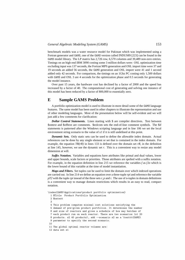
benchmark models was a water resource model for Pakistan which was implemented using aFortran generator andGAMS, one of theGAMS version called INDUS89 [223] can be found in theGAMS model library. The LP matrix has 2,726 row, 6,570 columns and 39,489 non-zero entries.Timings on an high end IBM 3090 costing some 3 million dollars were: OSL optimization timeexcluding input was 137 seconds, the Fortran MPS generation and OSL import time were 37 and19 seconds an added 56 seconds, theGAMS generation and OSL import were 41 and 1 secondadded only 42 seconds. For comparison, the timings on an 1Ghz PC costing only 1,500 dollarswith GAMS and OSL 3 are 4 seconds for the optimization phase and 0.5 seconds for generatingthe model instance.
Over past 15 years, the hardware cost has declined by a factor of 2000 and the speed hasincreased by a factor of 40. The computational cost of generating and solving one instance ofthis model has been reduced by a factor of 800,000 to essentially zero.
E Sample GAMS ProblemA portfolio optimization model is used to illustrate in more detail some of theGAMS language
features. The same model has been used in other chapters to illustrate the representation and useof other modeling languages. Most of the presentation below will be self-evident and we willjust add a few comments for clarification:
Dollar Control Statements.Lines starting with $ are compiler directives. Text between$ontext and $offtext are comments. $eolcom sets the end-of-line comment symbols. The $ifstatements is patterned after the Windows scripting language and in line 106 we set the localenvironment string scenario to the value ofs1 if it is still undefined at this point.
Dynamic Sets.Only static sets can be used to define the allowable index domain. Actualreferences can be done by any single element or set that is contained in the index domain. Forexample, the equationTR(rR) in lines 133 is defined over the domain setrR, in the definitionat line 145, however, we use the dynamic setr. This is a convenient way to resize any modeldimension at will.
Suffix Notation. Variables and equations have attributes like primal and dual values, lowerand upper bounds, scale factors or priorities. Those attributes are spefied with a suffix notation.For example, in the equation definition in line 215 we reference the variablesf asf.lo which isthe lower bound of this variable at the time of model instantiation.
Maps and Filters.Set tuples can be used to limit the domain over which indexed operationsare carried out. In line 214 we define an equation over a three-tuplerpi and reference the variablepT2with the tuplerpi insead of the three setsr, p andi. The use of n-tuples in domain definitionsis a convenient way to manage domain restrictions which results in an easy to read, compactnotation.
\index{GAMS!Applications!product portfolio optimization}1 $Title Product Portfolio Optimization2 $ontext34 This problem computes minimal cost solutions satisfying the5 demand of pre-given product portfolios. It determines the number6 and size of reactors and gives a schedule of how may batches of7 each product run on each reactor. There are two scenarios (s1 208 products. s2 40 products), add --scenario s2 as a \texttt{GAMS}9 parameter to specify the second scenario.
1011 The global optimal reactor volumes are:12 data set s1
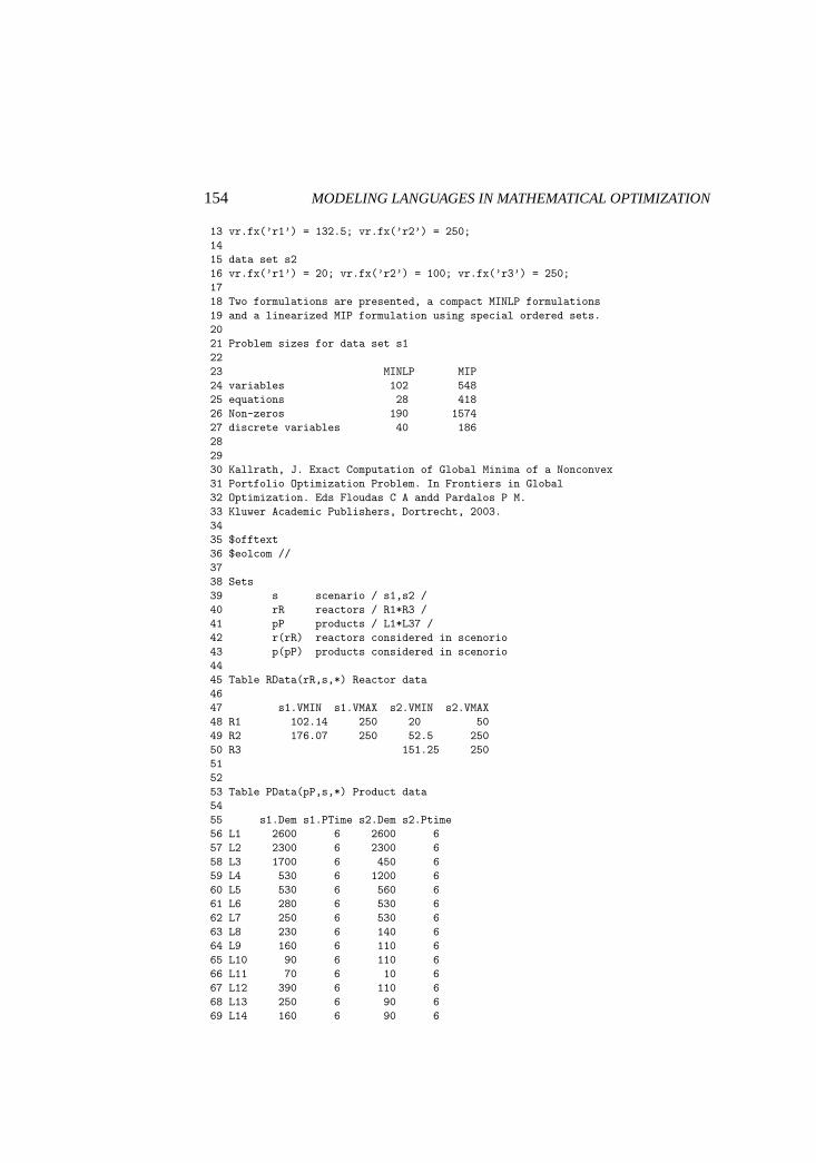
154 MODELING LANGUAGES IN MATHEMATICAL OPTIMIZATION
13 vr.fx(’r1’) = 132.5; vr.fx(’r2’) = 250;1415 data set s216 vr.fx(’r1’) = 20; vr.fx(’r2’) = 100; vr.fx(’r3’) = 250;1718 Two formulations are presented, a compact MINLP formulations19 and a linearized MIP formulation using special ordered sets.2021 Problem sizes for data set s12223 MINLP MIP24 variables 102 54825 equations 28 41826 Non-zeros 190 157427 discrete variables 40 186282930 Kallrath, J. Exact Computation of Global Minima of a Nonconvex31 Portfolio Optimization Problem. In Frontiers in Global32 Optimization. Eds Floudas C A andd Pardalos P M.33 Kluwer Academic Publishers, Dortrecht, 2003.3435 $offtext36 $eolcom //3738 Sets39 s scenario / s1,s2 /40 rR reactors / R1*R3 /41 pP products / L1*L37 /42 r(rR) reactors considered in scenorio43 p(pP) products considered in scenorio4445 Table RData(rR,s,*) Reactor data4647 s1.VMIN s1.VMAX s2.VMIN s2.VMAX48 R1 102.14 250 20 5049 R2 176.07 250 52.5 25050 R3 151.25 250515253 Table PData(pP,s,*) Product data5455 s1.Dem s1.PTime s2.Dem s2.Ptime56 L1 2600 6 2600 657 L2 2300 6 2300 658 L3 1700 6 450 659 L4 530 6 1200 660 L5 530 6 560 661 L6 280 6 530 662 L7 250 6 530 663 L8 230 6 140 664 L9 160 6 110 665 L10 90 6 110 666 L11 70 6 10 667 L12 390 6 110 668 L13 250 6 90 669 L14 160 6 90 6

General Algebraic Modeling System (GAMS) 155
70 L15 100 6 90 671 L16 70 6 70 672 L17 50 6 50 673 L18 50 6 30 674 L19 50 6 10 675 L20 10 676 L21 10 677 L22 190 678 L23 180 679 L24 70 680 L25 70 681 L26 40 682 L27 40 683 L28 40 684 L29 30 685 L30 20 686 L31 20 687 L32 20 688 L33 10 689 L34 10 690 L35 10 691 L36 10 692 L37 10 6939495 Parameters96 VMIN(rR) volume flow of products in m^3 per week97 VMAX(rR) volume flow of products in m^3 per week98 DEMAND(pP) volume flow of products in m^3 per week99 PRODTIME(pP) production time in hours per batch100 Scalars101 WHRS hours in a week / 168 /102 CSTI in kEuro depreciation per m^3 reactor and week / 0.97 /103 CSTF in kEuro per week and reactor / 2.45 /104 ESF economies of scale factor / 0.5 /;105106 $if not set scenario $set scenario s1107 VMIN(rR) = RDATA(rR,’%scenario%’,’VMIN’);108 VMAX(rR) = RDATA(rR,’%scenario%’,’VMAX’);109 DEMAND(pP) = PDATA(pP,’%scenario%’,’Dem’);110 PRODTIME(pP) = PDATA(pP,’%scenario%’,’PTime’);111112 * Determine scenario sets113 r(rR) = VMAX(rR) > 0;114 p(pP) = DEMAND(pP) > 0;115116 * definition of compact MINLP model117118 Variables cTotal total costs119 cInvest invest cost120 cFixed fix costs121 f(rR,pP) utilization rate122 vR(rR) reactor volume in m^3123 pS(pP) surplus production124 bvr(rR) indicating whether reactor r is active125 nB(rR,pP) number of batches of product p in reactor r126
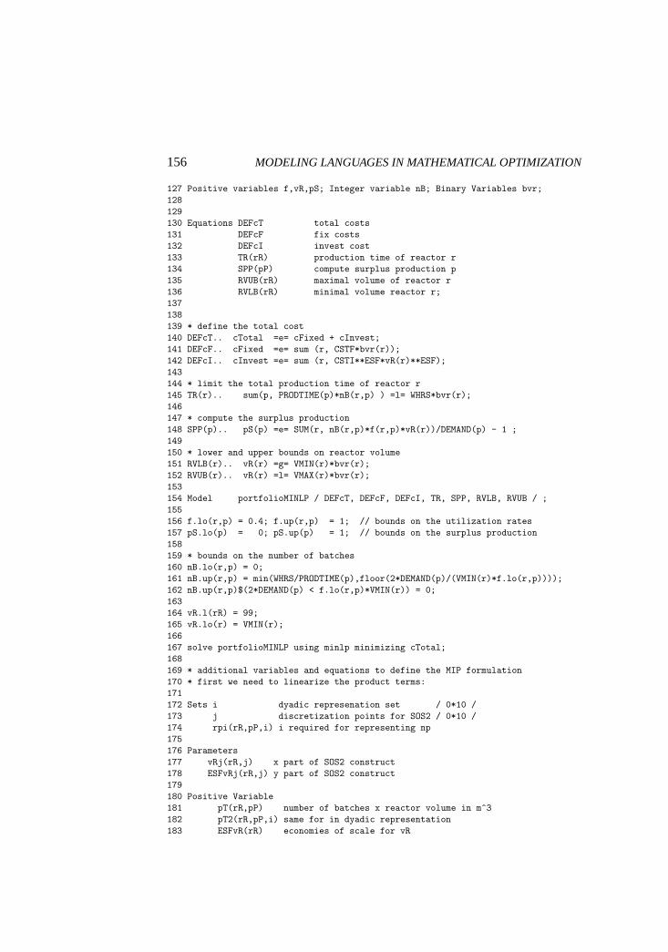
156 MODELING LANGUAGES IN MATHEMATICAL OPTIMIZATION
127 Positive variables f,vR,pS; Integer variable nB; Binary Variables bvr;128129130 Equations DEFcT total costs131 DEFcF fix costs132 DEFcI invest cost133 TR(rR) production time of reactor r134 SPP(pP) compute surplus production p135 RVUB(rR) maximal volume of reactor r136 RVLB(rR) minimal volume reactor r;137138139 * define the total cost140 DEFcT.. cTotal =e= cFixed + cInvest;141 DEFcF.. cFixed =e= sum (r, CSTF*bvr(r));142 DEFcI.. cInvest =e= sum (r, CSTI**ESF*vR(r)**ESF);143144 * limit the total production time of reactor r145 TR(r).. sum(p, PRODTIME(p)*nB(r,p) ) =l= WHRS*bvr(r);146147 * compute the surplus production148 SPP(p).. pS(p) =e= SUM(r, nB(r,p)*f(r,p)*vR(r))/DEMAND(p) - 1 ;149150 * lower and upper bounds on reactor volume151 RVLB(r).. vR(r) =g= VMIN(r)*bvr(r);152 RVUB(r).. vR(r) =l= VMAX(r)*bvr(r);153154 Model portfolioMINLP / DEFcT, DEFcF, DEFcI, TR, SPP, RVLB, RVUB / ;155156 f.lo(r,p) = 0.4; f.up(r,p) = 1; // bounds on the utilization rates157 pS.lo(p) = 0; pS.up(p) = 1; // bounds on the surplus production158159 * bounds on the number of batches160 nB.lo(r,p) = 0;161 nB.up(r,p) = min(WHRS/PRODTIME(p),floor(2*DEMAND(p)/(VMIN(r)*f.lo(r,p))));162 nB.up(r,p)$(2*DEMAND(p) < f.lo(r,p)*VMIN(r)) = 0;163164 vR.l(rR) = 99;165 vR.lo(r) = VMIN(r);166167 solve portfolioMINLP using minlp minimizing cTotal;168169 * additional variables and equations to define the MIP formulation170 * first we need to linearize the product terms:171172 Sets i dyadic represenation set / 0*10 /173 j discretization points for SOS2 / 0*10 /174 rpi(rR,pP,i) i required for representing np175176 Parameters177 vRj(rR,j) x part of SOS2 construct178 ESFvRj(rR,j) y part of SOS2 construct179180 Positive Variable181 pT(rR,pP) number of batches x reactor volume in m^3182 pT2(rR,pP,i) same for in dyadic representation183 ESFvR(rR) economies of scale for vR
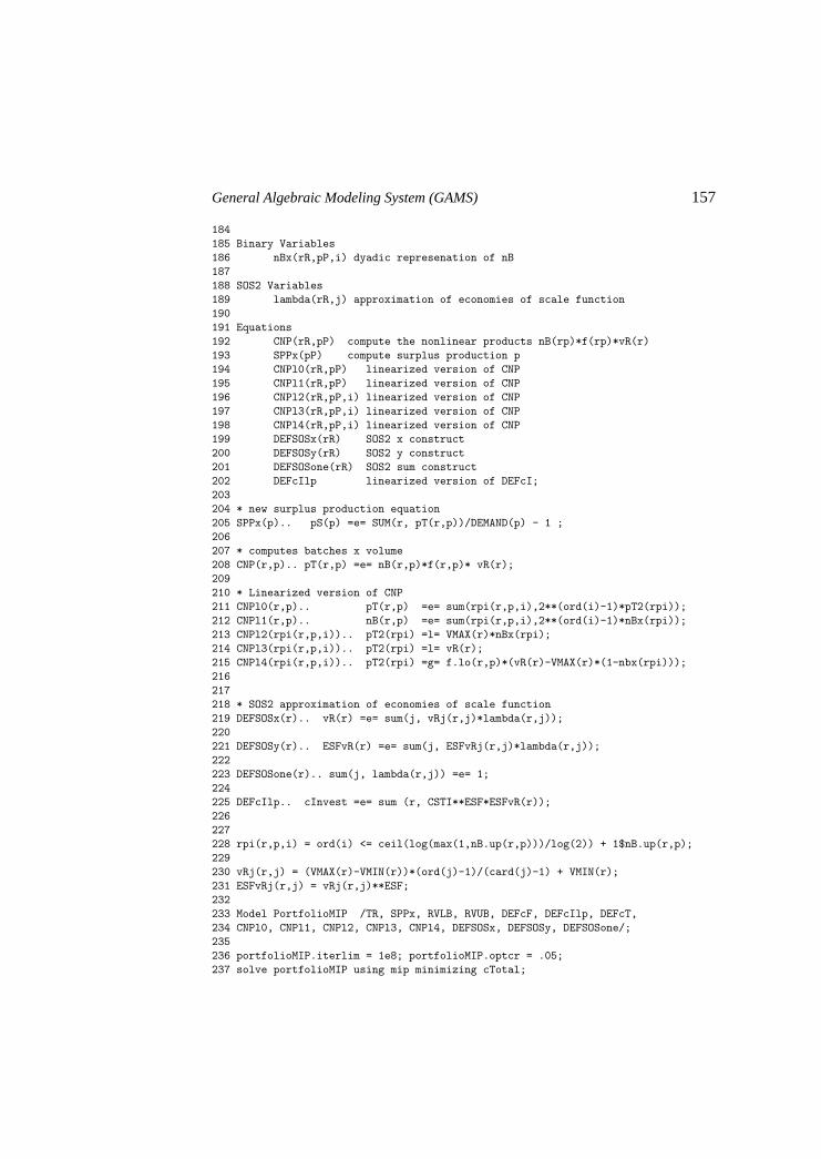
General Algebraic Modeling System (GAMS) 157
184185 Binary Variables186 nBx(rR,pP,i) dyadic represenation of nB187188 SOS2 Variables189 lambda(rR,j) approximation of economies of scale function190191 Equations192 CNP(rR,pP) compute the nonlinear products nB(rp)*f(rp)*vR(r)193 SPPx(pP) compute surplus production p194 CNPl0(rR,pP) linearized version of CNP195 CNPl1(rR,pP) linearized version of CNP196 CNPl2(rR,pP,i) linearized version of CNP197 CNPl3(rR,pP,i) linearized version of CNP198 CNPl4(rR,pP,i) linearized version of CNP199 DEFSOSx(rR) SOS2 x construct200 DEFSOSy(rR) SOS2 y construct201 DEFSOSone(rR) SOS2 sum construct202 DEFcIlp linearized version of DEFcI;203204 * new surplus production equation205 SPPx(p).. pS(p) =e= SUM(r, pT(r,p))/DEMAND(p) - 1 ;206207 * computes batches x volume208 CNP(r,p).. pT(r,p) =e= nB(r,p)*f(r,p)* vR(r);209210 * Linearized version of CNP211 CNPl0(r,p).. pT(r,p) =e= sum(rpi(r,p,i),2**(ord(i)-1)*pT2(rpi));212 CNPl1(r,p).. nB(r,p) =e= sum(rpi(r,p,i),2**(ord(i)-1)*nBx(rpi));213 CNPl2(rpi(r,p,i)).. pT2(rpi) =l= VMAX(r)*nBx(rpi);214 CNPl3(rpi(r,p,i)).. pT2(rpi) =l= vR(r);215 CNPl4(rpi(r,p,i)).. pT2(rpi) =g= f.lo(r,p)*(vR(r)-VMAX(r)*(1-nbx(rpi)));216217218 * SOS2 approximation of economies of scale function219 DEFSOSx(r).. vR(r) =e= sum(j, vRj(r,j)*lambda(r,j));220221 DEFSOSy(r).. ESFvR(r) =e= sum(j, ESFvRj(r,j)*lambda(r,j));222223 DEFSOSone(r).. sum(j, lambda(r,j)) =e= 1;224225 DEFcIlp.. cInvest =e= sum (r, CSTI**ESF*ESFvR(r));226227228 rpi(r,p,i) = ord(i) <= ceil(log(max(1,nB.up(r,p)))/log(2)) + 1$nB.up(r,p);229230 vRj(r,j) = (VMAX(r)-VMIN(r))*(ord(j)-1)/(card(j)-1) + VMIN(r);231 ESFvRj(r,j) = vRj(r,j)**ESF;232233 Model PortfolioMIP /TR, SPPx, RVLB, RVUB, DEFcF, DEFcIlp, DEFcT,234 CNPl0, CNPl1, CNPl2, CNPl3, CNPl4, DEFSOSx, DEFSOSy, DEFSOSone/;235236 portfolioMIP.iterlim = 1e8; portfolioMIP.optcr = .05;237 solve portfolioMIP using mip minimizing cTotal;