chapter 7 'support vector machines for pattern recognition
TRANSCRIPT
7 Pattern Recognition
This chapter is devoted to a detailed description of SV classification (SVC) meth-ods. We have already briefly visited the SVC algorithm in Chapter 1. There will besome overlap with that chapter, but here we give a more thorough treatment.We start by describing the classifier that forms the basis for SVC, the separatingOverview
hyperplane (Section 7.1). Separating hyperplanes can differ in how large a marginof separation they induce between the classes, with corresponding consequenceson the generalization error, as discussed in Section 7.2. The “optimal” margin hy-perplane is defined in Section 7.3, along with a description of how to compute it.Using the kernel trick of Chapter 2, we generalize to the case where the optimalmargin hyperplane is not computed in input space, but in a feature space nonlin-early related to the latter (Section 7.4). This dramatically increases the applicabilityof the approach, as does the introduction of slack variables to deal with outliersand noise in the data (Section 7.5). Many practical problems require us to classifythe data into more than just two classes. Section 7.6 describes how multi-class SVclassification systems can be built. Following this, Section 7.7 describes some vari-ations on standard SV classification algorithms, differing in the regularizers andconstraints that are used. We conclude with a fairly detailed section on experi-ments and applications (Section 7.8).This chapter requires basic knowledge of kernels, as conveyed in the first halfPrerequisites
of Chapter 2. To understand details of the optimization problems, it is helpful (butnot indispensable) to get some background from Chapter 6. To understand theconnections to learning theory, in particular regarding the statistical basis of theregularizer used in SV classification, it would be useful to have read Chapter 5.
7.1 Separating Hyperplanes
Suppose we are given a dot product space �, and a set of pattern vectorsx1� � � � � xm ��. Any hyperplane in� can be written asHyperplane
�x ��� �w� x�� b � 0�� w ��� b � � � (7.1)
In this formulation, w is a vector orthogonal to the hyperplane: If w has unitlength, then �w� x� is the length of x along the direction of w (Figure 7.1). Forgeneral w, this number will be scaled by �w�. In any case, the set (7.1) consists
190 Pattern Recognition
7.8 Experiments
7.2 Margins
7.3 Optimal MarginHyperplane
6 Optimization
7.4 Optimal MarginBinary Classifiers
7.5 Soft MarginBinary Classifiers
Classifiers7.6 Multi−Class
7.1 SeparatingHyperplane
7.7 Variations
2 Kernels
of vectors that all have the same length along w. In other words, these are vectorsthat project onto the same point on the line spanned by w.In this formulation, we still have the freedom to multiply w and b by the same
non-zero constant. This superfluous freedom— physicists would call it a “gauge”freedom— can be abolished as follows.
Definition 7.1 (Canonical Hyperplane) The pair (w� b)���� is called a canonicalform of the hyperplane (7.1) with respect to x1� � � � � xm ��, if it is scaled such that
mini�1�����m
� �w� xi�� b� � 1� (7.2)
which amounts to saying that the point closest to the hyperplane has a distance of 1��w�(Figure 7.2).
Note that the condition (7.2) still allows two such pairs: given a canonical hyper-plane (w� b), another one satisfying (7.2) is given by (w�b). For the purpose ofpattern recognition, these two hyperplanes turn out to be different, as they areoriented differently; they correspond to two decision functions,Decision
Functionfw�b :� ��1�
x � fw�b(x) � sgn��w� x�� b
�� (7.3)
which are the inverse of each other.In the absence of class labels yi � ��1� associated with the xi, there is no way
of distinguishing the two hyperplanes. For a labelled dataset, a distinction exists:The two hyperplanes make opposite class assignments. In pattern recognition,
7.1 Separating Hyperplanes 191
w
◆
◆
◆
◆
●●
●
●● {x | <w x> + b = 0},
<w x> + b > 0,
<w x> + b < 0,
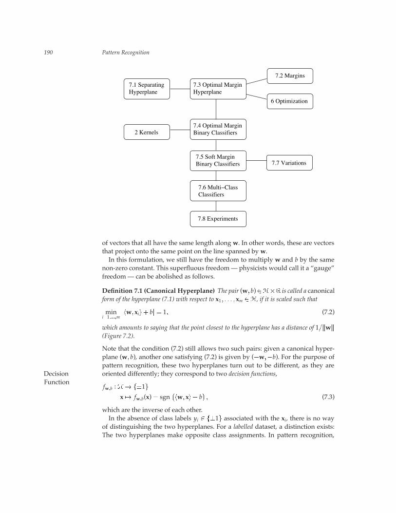
Figure 7.1 A separable classification problem, alongwith a separating hyperplane, writtenin terms of an orthogonal weight vectorw and a threshold b. Note that by multiplying bothw and b by the same non-zero constant, we obtain the same hyperplane, represented interms of different parameters. Figure 7.2 shows how to eliminate this scaling freedom.
,w
{x | <w x> + b = 0},
{x | <w x> + b = −1},{x | <w x> + b = +1},
x2x1
Note:
<w x1> + b = +1<w x2> + b = −1
=> <w (x1−x2)> = 2
=> (x1−x2) =w
||w||< >
,,
,
, 2||w||
yi = −1
yi = +1❍❍
❍
❍❍
◆
◆
◆
◆
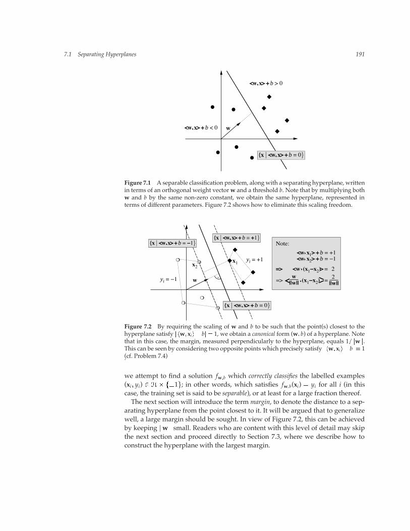
Figure 7.2 By requiring the scaling of w and b to be such that the point(s) closest to thehyperplane satisfy � �w�xi�� b� � 1, we obtain a canonical form (w� b) of a hyperplane. Notethat in this case, the margin, measured perpendicularly to the hyperplane, equals 1��w�.This can be seen by considering two opposite points which precisely satisfy � �w�xi�� b�� 1(cf. Problem 7.4).
we attempt to find a solution fw�b which correctly classifies the labelled examples(xi� yi) � �� ��1�; in other words, which satisfies fw�b(xi) � yi for all i (in thiscase, the training set is said to be separable), or at least for a large fraction thereof.The next section will introduce the term margin, to denote the distance to a sep-
arating hyperplane from the point closest to it. It will be argued that to generalizewell, a large margin should be sought. In view of Figure 7.2, this can be achievedby keeping �w� small. Readers who are content with this level of detail may skipthe next section and proceed directly to Section 7.3, where we describe how toconstruct the hyperplane with the largest margin.
192 Pattern Recognition
7.2 The Role of the Margin
Themargin plays a crucial role in the design of SV learning algorithms. Let us startby formally defining it.
Definition 7.2 (Geometrical Margin) For a hyperplane �x � �� �w� x�� b � 0�, wecall
�(w�b)(x� y) :� y(�w� x�� b)��w� (7.4)
the geometrical margin of the point (x� y) �����1�. The minimum valueGeometricalMargin
�(w�b) :� mini�1�����m
�(w�b)(xi� yi) (7.5)
shall be called the geometrical margin of (x1� y1)� � � � � (xm� ym). If the latter is omitted, itis understood that the training set is meant.
Occasionally, we will omit the qualification geometrical, and simply refer to themargin.For a point (x� y) which is correctly classified, the margin is simply the distance
from x to the hyperplane. To see this, note first that the margin is zero on thehyperplane. Second, in the definition, we effectively consider a hyperplane
(w� b) :� (w��w�� b��w�)� (7.6)
which has a unit lengthweight vector, and then compute the quantity y(�w� x�� b).The term �w� x�, however, simply computes the length of the projection of x ontothe direction orthogonal to the hyperplane, which, after adding the offset b, equalsthe distance to it. The multiplication by y ensures that the margin is positivewhenever a point is correctly classified. For misclassified points, we thus get amargin which equals the negative distance to the hyperplane. Finally, note thatfor canonical hyperplanes, the margin is 1��w� (Figure 7.2). The definition ofMargin of
CanonicalHyperplanes
the canonical hyperplane thus ensures that the length of w now corresponds toa meaningful geometrical quantity.It turns out that the margin of a separating hyperplane, and thus the length of
the weight vector w, plays a fundamental role in support vector type algorithms.Loosely speaking, if we manage to separate the training data with a large margin,thenwe have reason to believe that wewill dowell on the test set. Not surprisingly,there exist a number of explanations for this intuition, ranging from the simple tothe rather technical. We will now briefly sketch some of them.The simplest possible justification for large margins is as follows. Since theInsensitivity to
Pattern Noise training and test data are assumed to have been generated by the same underlyingdependence, it seems reasonable to assume that most of the test patterns will lieclose (in�) to at least one of the training patterns. For the sake of simplicity, let usconsider the case where all test points are generated by adding bounded patternnoise (sometimes called input noise) to the training patterns. More precisely, givena training point (x� y), we will generate test points of the form (x� ∆x� y), where
7.2 The Role of the Margin 193
o
o
o
+
+
+
o
+
r
ρ
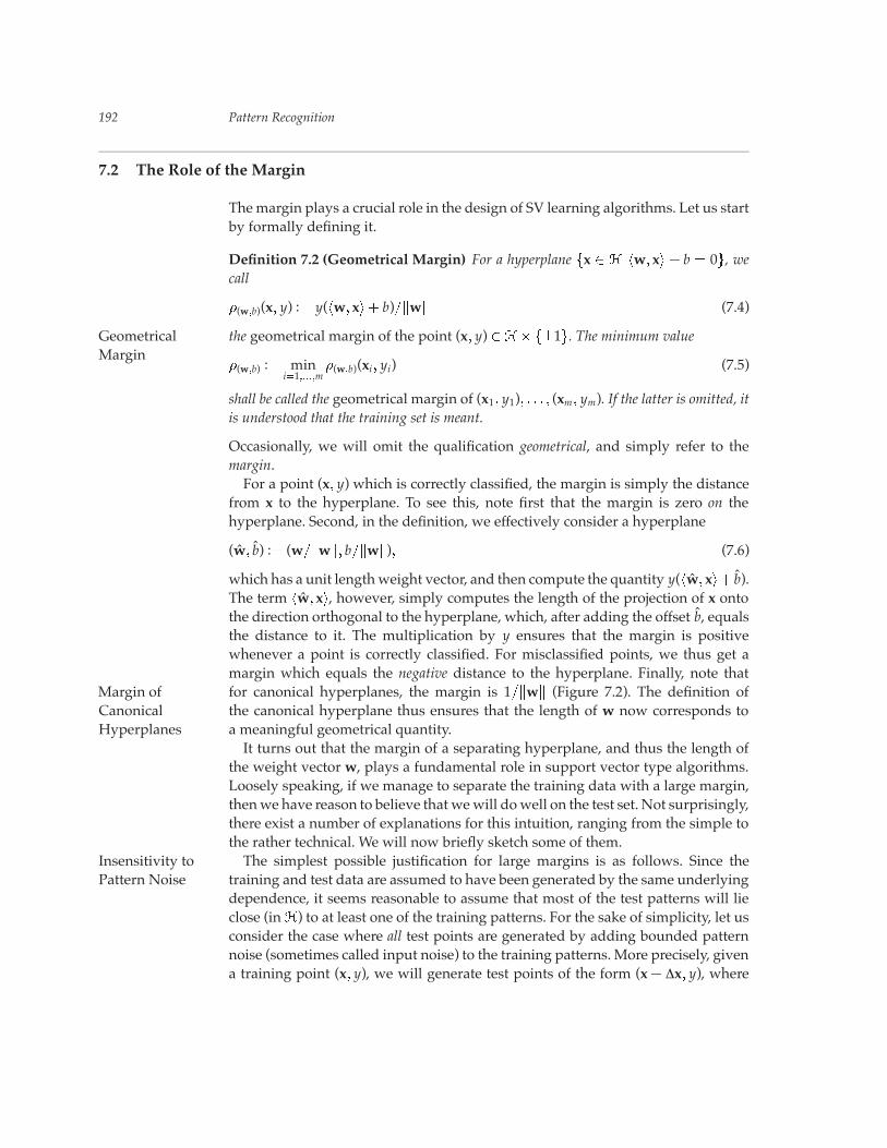
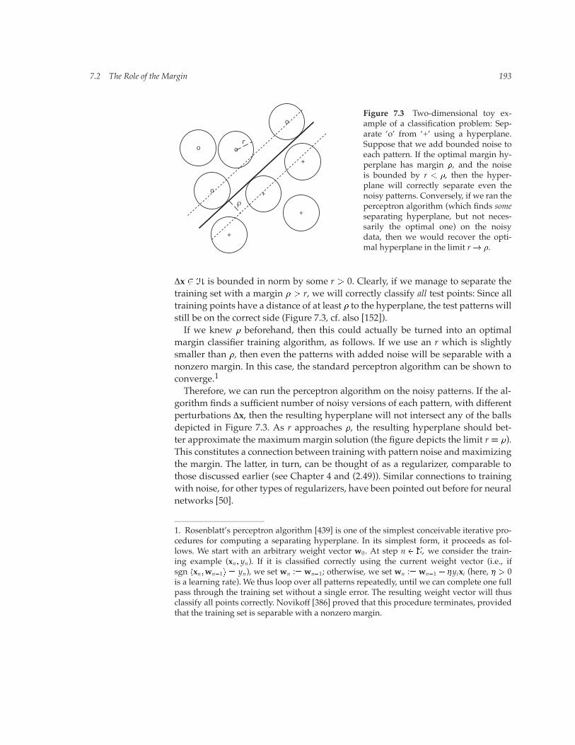
Figure 7.3 Two-dimensional toy ex-ample of a classification problem: Sep-arate ‘o’ from ‘+’ using a hyperplane.Suppose that we add bounded noise toeach pattern. If the optimal margin hy-perplane has margin �, and the noiseis bounded by r � �, then the hyper-plane will correctly separate even thenoisy patterns. Conversely, if we ran theperceptron algorithm (which finds someseparating hyperplane, but not neces-sarily the optimal one) on the noisydata, then we would recover the opti-mal hyperplane in the limit r� �.
∆x � � is bounded in norm by some r � 0. Clearly, if we manage to separate thetraining set with a margin � � r, we will correctly classify all test points: Since alltraining points have a distance of at least � to the hyperplane, the test patterns willstill be on the correct side (Figure 7.3, cf. also [152]).If we knew � beforehand, then this could actually be turned into an optimal
margin classifier training algorithm, as follows. If we use an r which is slightlysmaller than �, then even the patterns with added noise will be separable with anonzero margin. In this case, the standard perceptron algorithm can be shown toconverge.1
Therefore, we can run the perceptron algorithm on the noisy patterns. If the al-gorithm finds a sufficient number of noisy versions of each pattern, with differentperturbations ∆x, then the resulting hyperplane will not intersect any of the ballsdepicted in Figure 7.3. As r approaches �, the resulting hyperplane should bet-ter approximate the maximummargin solution (the figure depicts the limit r � �).This constitutes a connection between training with pattern noise andmaximizingthe margin. The latter, in turn, can be thought of as a regularizer, comparable tothose discussed earlier (see Chapter 4 and (2.49)). Similar connections to trainingwith noise, for other types of regularizers, have been pointed out before for neuralnetworks [50].
1. Rosenblatt’s perceptron algorithm [439] is one of the simplest conceivable iterative pro-cedures for computing a separating hyperplane. In its simplest form, it proceeds as fol-lows. We start with an arbitrary weight vector w0. At step n � � , we consider the train-ing example (xn� yn). If it is classified correctly using the current weight vector (i.e., ifsgn �xn�wn�1� � yn), we set wn :� wn�1; otherwise, we set wn :� wn�1 � �yixi (here, � � 0is a learning rate). We thus loop over all patterns repeatedly, until we can complete one fullpass through the training set without a single error. The resulting weight vector will thusclassify all points correctly. Novikoff [386] proved that this procedure terminates, providedthat the training set is separable with a nonzero margin.
194 Pattern Recognition
o
o
o
+
+
+
o
+γ+∆γ
γ
Rρ
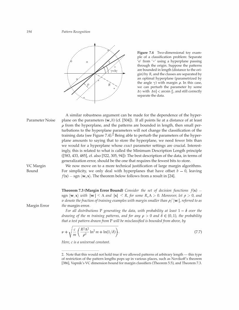
Figure 7.4 Two-dimensional toy exam-ple of a classification problem: Separate‘o’ from ‘+’ using a hyperplane passingthrough the origin. Suppose the patternsare bounded in length (distance to the ori-gin) by R, and the classes are separated byan optimal hyperplane (parametrized bythe angle �) with margin �. In this case,we can perturb the parameter by some∆� with �∆��� arcsin �
R , and still correctlyseparate the data.
A similar robustness argument can be made for the dependence of the hyper-plane on the parameters (w� b) (cf. [504]). If all points lie at a distance of at leastParameter Noise� from the hyperplane, and the patterns are bounded in length, then small per-turbations to the hyperplane parameters will not change the classification of thetraining data (see Figure 7.4).2 Being able to perturb the parameters of the hyper-plane amounts to saying that to store the hyperplane, we need fewer bits thanwe would for a hyperplane whose exact parameter settings are crucial. Interest-ingly, this is related to what is called the Minimum Description Length principle([583, 433, 485], cf. also [522, 305, 94]): The best description of the data, in terms ofgeneralization error, should be the one that requires the fewest bits to store.We now move on to a more technical justification of large margin algorithms.VC Margin
Bound For simplicity, we only deal with hyperplanes that have offset b � 0, leavingf (x) � sgn �w� x�. The theorem below follows from a result in [24].
Theorem 7.3 (Margin Error Bound) Consider the set of decision functions f (x) �sgn �w� x� with �w� Λ and �x� R, for some R�Λ � 0. Moreover, let � � 0, and� denote the fraction of training examples with margin smaller than ���w�, referred to asthemargin error.Margin ErrorFor all distributions P generating the data, with probability at least 1 � Æ over the
drawing of the m training patterns, and for any � � 0 and Æ � (0� 1), the probabilitythat a test pattern drawn from P will be misclassified is bounded from above, by
� �
�cm
�R2Λ2
�2ln2m� ln(1�Æ)
�� (7.7)
Here, c is a universal constant.
2. Note that this would not hold true if we allowed patterns of arbitrary length — this typeof restriction of the pattern lengths pops up in various places, such as Novikoff’s theorem[386], Vapnik’s VC dimension bound for margin classifiers (Theorem 5.5), and Theorem 7.3.
7.2 The Role of the Margin 195
Let us try to understand this theorem. It makes a probabilistic statement about aprobability, by giving an upper bound on the probability of test error, which itselfonly holds true with a certain probability, 1� Æ. Where do these two probabilitiescome from? The first is due to the fact that the test examples are randomly drawnfrom P; the second is due to the training examples being drawn from P. Strictlyspeaking, the bound does not refer to a single classifier that has been trained onsome fixed data set at hand, but to an ensemble of classifiers, trained on variousinstantiations of training sets generated by the same underlying regularity P.It is beyond the scope of the present chapter to prove this result. The basic ingre-
dients of bounds of this type, commonly referred to as VC bounds, are describedin Chapter 5; for further details, see Chapter 12, and [562, 491, 504, 125]. Severalaspects of the bound are noteworthy. The test error is bounded by a sum of themargin error � , and a capacity term (the �� � � term in (7.7)), with the latter tend-ing to zero as the number of examples, m, tends to infinity. The capacity term canbe kept small by keeping R and Λ small, and making � large. If we assume thatR and Λ are fixed a priori, the main influence is �. As can be seen from (7.7), alarge � leads to a small capacity term, but the margin error � gets larger. A small�, on the other hand, will usually cause fewer points to have margins smaller than���w�, leading to a smaller margin error; but the capacity penalty will increasecorrespondingly. The overall message: Try to find a hyperplane which is alignedsuch that even for a large �, there are few margin errors.Maximizing �, however, is the same as minimizing the length of w. Hence we
might just as well keep � fixed, say, equal to 1 (which is the case for canonicalhyperplanes), and search for a hyperplane which has a small �w� and few pointswith a margin smaller than 1��w�; in other words (Definition 7.2), few points suchthat y �w� x� � 1.It should be emphasized that dropping the condition �w� Λ would prevent
us from stating a bound of the kind shown above. We could give an alternativebound, where the capacity depends on the dimensionality of the space �. Thecrucial advantage of the bound given above is that it is independent of thatdimensionality, enabling us to work in very high dimensional spaces. This willbecome important when we make use of the kernel trick.It has recently been pointed out that the margin also plays a crucial role in im-
proving asymptotic rates in nonparametric estimation [551]. This topic, however,is beyond the scope of the present book.To conclude this section, we note that large margin classifiers also have advan-Implementation
in Hardware tages of a practical nature: An algorithm that can separate a dataset with a certainmargin will behave in a benign way when implemented in hardware. Real-worldsystems typically work only within certain accuracy bounds, and if the classifieris insensitive to small changes in the inputs, it will usually tolerate those inaccura-cies.We have thus accumulated a fair amount of evidence in favor of the following
approach: Keep the margin training error small, and the margin large, in order toachieve high generalization ability. In other words, hyperplane decision functions
196 Pattern Recognition
should be constructed such that they maximize the margin, and at the same timeseparate the training data with as few exceptions as possible. Sections 7.3 and 7.5respectively will deal with these two issues.
7.3 Optimal Margin Hyperplanes
Let us now derive the optimization problem to be solved for computing the opti-mal hyperplane. Suppose we are given a set of examples (x1� y1)� � � � � (xm� ym)� xi ��� yi � �1�. Here and below, the index i runs over 1� � � � �m by default. We assumethat there is at least one negative and one positive yi. We want to find a decisionfunction fw�b(x) � sgn
��w� x�� b� satisfyingfw�b(xi) � yi� (7.8)
If such a function exists (the non-separable case will be dealt with later), canoni-cality (7.2) implies
yi��xi�w�� b� 1� (7.9)
As an aside, note that out of the two canonical forms of the same hyperplane, (w� b)and (�w��b), only one will satisfy equations (7.8) and (7.11). The existence of classlabels thus allows to distinguish two orientations of a hyperplane.Following the previous section, a separating hyperplane which generalizes well
can thus be constructed by solving the following problem:
minimizew���b��
� (w) �12�w�2� (7.10)
subject to yi��xi�w�� b� 1 for all i � 1� � � � �m� (7.11)
This is called the primal optimization problem.Problems like this one are the subject of optimization theory. For details on how
to solve them, see Chapter 6; for a short intuitive explanation, cf. the remarksfollowing (1.26) in the introductory chapter. We will now derive the so-called dualproblem, which can be shown to have the same solutions as (7.10). In the presentcase, it will turn out that it is more convenient to deal with the dual. To derive it,we introduce the Lagrangian,Lagrangian
L(w� b��) �12�w�2 �
m
∑i�1
i�yi(�xi�w�� b)� 1
�� (7.12)
with Lagrange multipliers i 0. Recall that as in Chapter 1, we use bold faceGreek variables to refer to the corresponding vectors of variables, for instance,� � (1� � � � � m).The Lagrangian L must be maximized with respect to i, and minimized with
respect to w and b (see Theorem 6.26). Consequently, at this saddle point, the
7.3 Optimal Margin Hyperplanes 197
derivatives of L with respect to the primal variables must vanish,
�
�bL(w� b��) � 0�
�
�wL(w� b��) � 0� (7.13)
which leads tom
∑i�1
�i yi � 0� (7.14)
and
w �m
∑i�1
�i yixi� (7.15)
The solution vector thus has an expansion in terms of training examples. Notethat although the solution w is unique (due to the strict convexity of (7.10), andthe convexity of (7.11)), the coefficients �i need not be.According to the KKT theorem (Chapter 6), only the Lagrange multipliers �i
that are non-zero at the saddle point, correspond to constraints (7.11) which areprecisely met. Formally, for all i � 1� � � � �m, we have
�i[yi(�xi�w�� b)� 1] � 0� (7.16)
The patterns xi for which �i � 0 are called Support Vectors. This terminology isSupport Vectorsrelated to corresponding terms in the theory of convex sets, relevant to convexoptimization (e.g., [334, 45]).3 According to (7.16), they lie exactly on the margin.4
All remaining examples in the training set are irrelevant: Their constraints (7.11)are satisfied automatically, and they do not appear in the expansion (7.15), sincetheir multipliers satisfy �i � 0.5
This leads directly to an upper bound on the generalization ability of optimalmargin hyperplanes. To this end, we consider the so-called leave-one-out method(for further details, see Section 12.2) to estimate the expected test error [335, 559].This procedure is based on the idea that if we leave out one of the training
3. Given any boundary point of a convex set, there always exists a hyperplane separatingthe point from the interior of the set. This is called a supporting hyperplane.SVs lie on the boundary of the convex hulls of the two classes, thus they possess support-
ing hyperplanes. The SV optimal hyperplane is the hyperplane which lies in the middle ofthe two parallel supporting hyperplanes (of the two classes) with maximum distance.Conversely, from the optimal hyperplane, we can obtain supporting hyperplanes for all
SVs of both classes, by shifting it by 1��w� in both directions.4. Note that this implies the solution (w� b), where b is computed using yi(�w�xi�� b)� 1 forSVs, is in canonical formwith respect to the training data. (This makes use of the reasonableassumption that the training set contains both positive and negative examples.)5. In a statistical mechanics framework, Anlauf and Biehl [12] have put forward a similarargument for the optimal stability perceptron, also computed using constrained optimization.There is a large body of work in the physics community on optimal margin classification.Some further references of interest are [310, 191, 192, 394, 449, 141]; other early worksinclude [313].
198 Pattern Recognition
examples, and train on the remaining ones, then the probability of error on the leftout example gives us a fair indication of the true test error. Of course, doing this fora single training example leads to an error of either zero or one, so it does not yetgive an estimate of the test error. The leave-one-out method repeats this procedurefor each individual training example in turn, and averages the resulting errors.Let us return to the present case. If we leave out a pattern xi� , and construct
the solution from the remaining patterns, the following outcomes are possible (cf.(7.11)):
1. yi���xi� �w�� b
�� 1. In this case, the pattern is classified correctly and does not
lie on the margin. These are patterns that would not have become SVs anyway.
2. yi���xi� �w�� b
�� 1. In other words, xi� exactly meets the constraint (7.11). In
this case, the solution w does not change, even though the coefficients �i wouldchange: Namely, if xi� might have become a Support Vector (i.e., �i� � 0) hadit been kept in the training set. In that case, the fact that the solution is thesame, no matter whether xi� is in the training set or not, means that xi� can bewritten as ∑SVs �i yixi with, �i � 0. Note that condition 2 is not equivalent to sayingthat xi� may be written as some linear combination of the remaining SupportVectors: Since the sign of the coefficients in the linear combination is determinedby the class of the respective pattern, not any linear combination will do. Strictlyspeaking, xi� must lie in the cone spanned by the yixi, where the xi are all SupportVectors.6 For more detail, see [565] and Section 12.2.
3. 0 � yi���xi� �w�� b
�� 1. In this case, xi� lies within the margin, but still on the
correct side of the decision boundary. Thus, the solution looks different from theone obtained with xi� in the training set (in that case, xi� would satisfy (7.11) aftertraining); classification is nevertheless correct.
4. yi���xi� �w�� b
�� 0. This means that xi� is classified incorrectly.
Note that cases 3 and 4 necessarily correspond to examples which would havebecome SVs if kept in the training set; case 2 potentially includes such situations.Only case 4, however, leads to an error in the leave-one-out procedure. Conse-quently, we have the following result on the generalization error of optimal mar-gin classifiers [570]:7
Proposition 7.4 The expectation of the number of Support Vectors obtained during train-Leave-One-OutBound ing on a training set of size m, divided by m, is an upper bound on the expected proba-
bility of test error of the SVM trained on training sets of size m� 1.8
6. Possible non-uniqueness of the solution’s expansion in terms of SVs is related to zeroEigenvalues of (yiyjk(xi� xj))i j, cf. Proposition 2.16. Note, however, the above caveat on thedistinction between linear combinations, and linear combinations with coefficients of fixedsign.7. It also holds for the generalized versions of optimal margin classifiers described in thefollowing sections.8. Note that the leave-one-out procedure performed with m training examples thus yields
7.3 Optimal Margin Hyperplanes 199
.w
◆
◆
◆
◆
●●
●
●● {x | <w x> + b = 0},
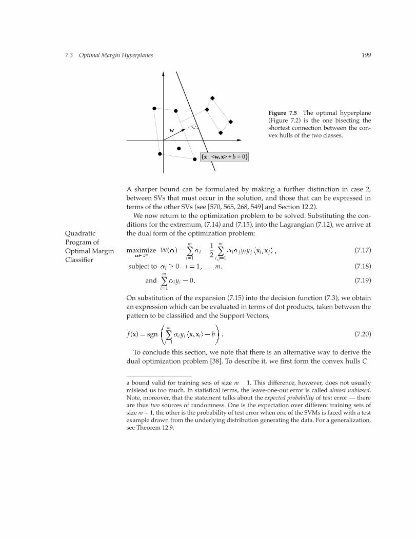
Figure 7.5 The optimal hyperplane(Figure 7.2) is the one bisecting theshortest connection between the con-vex hulls of the two classes.
A sharper bound can be formulated by making a further distinction in case 2,between SVs that must occur in the solution, and those that can be expressed interms of the other SVs (see [570, 565, 268, 549] and Section 12.2).We now return to the optimization problem to be solved. Substituting the con-
ditions for the extremum, (7.14) and (7.15), into the Lagrangian (7.12), we arrive atthe dual form of the optimization problem:Quadratic
Program ofOptimal MarginClassifier
maximize���m
W(�) �m
∑i�1
�i �12
m
∑i� j�1
�i� j yiy j�xi� x j
�� (7.17)
subject to �i � 0� i � 1� � � � �m� (7.18)
andm
∑i�1
�i yi � 0� (7.19)
On substitution of the expansion (7.15) into the decision function (7.3), we obtainan expression which can be evaluated in terms of dot products, taken between thepattern to be classified and the Support Vectors,
f (x) � sgn
�m
∑i�1
�i yi �x� xi�� b
�� (7.20)
To conclude this section, we note that there is an alternative way to derive thedual optimization problem [38]. To describe it, we first form the convex hulls C�
a bound valid for training sets of size m � 1. This difference, however, does not usuallymislead us too much. In statistical terms, the leave-one-out error is called almost unbiased.Note, moreover, that the statement talks about the expected probability of test error — thereare thus two sources of randomness. One is the expectation over different training sets ofsizem� 1, the other is the probability of test error when one of the SVMs is faced with a testexample drawn from the underlying distribution generating the data. For a generalization,see Theorem 12.9.
200 Pattern Recognition
and C� of both classes of training points,
C� :�
�∑yi��1
cixi
����� ∑yi��1 ci � 1� ci � 0� (7.21)
It can be shown that the maximum margin hyperplane as described above is theConvex HullSeparation one bisecting the shortest line orthogonally connecting C� and C� (Figure 7.5).
Formally, this can be seen by considering the optimization problem
minimizec��m
∑yi�1 cixi � ∑yi��1
cixi
2
�
subject to ∑yi�1
ci � 1� ∑yi��1
ci � 1� ci � 0� (7.22)
and using the normal vectorw�∑yi�1 cixi�∑yi��1 cixi, scaled to satisfy the canon-icality condition (Definition 7.1). The threshold b is explicitly adjusted such that thehyperplane bisects the shortest connecting line (see also Problem 7.7).
7.4 Nonlinear Support Vector Classifiers
Thus far, we have shown why it is that a large margin hyperplane is good from astatistical point of view, and we have demonstrated how to compute it. Althoughthese two points have worked out nicely, there is still a major drawback to theapproach: Everything that we have done so far is linear in the data. To allowfor much more general decision surfaces, we now use kernels to nonlinearlytransform the input data x1� � � � � xm � � into a high-dimensional feature space,using a map Φ : xi � xi; we then do a linear separation there.To justify this procedure, Cover’s Theorem [113] is sometimes alluded to. This
theorem characterizes the number of possible linear separations of m points ingeneral position in an N-dimensional space. If m � N� 1, then all 2m separationsare possible — the VC dimension of the function class is n� 1 (Section 5.5.6). Ifm � N � 1, then Cover’s Theorem states that the number of linear separationsCover’s Theoremequals
2N
∑i�0
�m� 1
i
�� (7.23)
The more we increase N, the more terms there are in the sum, and thus the largeris the resulting number. This theorem formalizes the intuition that the number ofseparations increases with the dimensionality. It requires, however, that the pointsare in general position — therefore, it does not strictly make a statement aboutthe separability of a given dataset in a given feature space. E.g., the feature mapmight be such that all points lie on a rather restrictive lower-dimensionalmanifold,which could prevent us from finding points in general position.There is another way to intuitively understand why the kernel mapping in-
7.4 Nonlinear Support Vector Classifiers 201
R3
✕
❍
❍
✕
✕
✕
R2
✕
✕
✕
✕
❍
❍
R2
✕
✕
✕
✕
❍
❍
Φ
Φ:R2 R3
x1 x2
w1w2 w3
f (x)
input space
feature space2 x1x2 x12 x2
2
f (x)=sgn (w1x1+w2x2+w3 2 x1x2+b)2 2
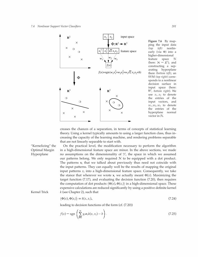
Figure 7.6 By map-ping the input data(top left) nonlin-early (via Φ) into ahigher-dimensionalfeature space �
(here: � � �3 ), and
constructing a sep-arating hyperplanethere (bottom left), anSVM (top right) corre-sponds to a nonlineardecision surface ininput space (here:�2 , bottom right). Weuse x1� x2 to denotethe entries of theinput vectors, andw1�w2�w3 to denotethe entries of thehyperplane normalvector in�.
creases the chances of a separation, in terms of concepts of statistical learningtheory. Using a kernel typically amounts to using a larger function class, thus in-creasing the capacity of the learning machine, and rendering problems separablethat are not linearly separable to start with.On the practical level, the modification necessary to perform the algorithm“Kernelizing” the
Optimal MarginHyperplane
in a high-dimensional feature space are minor. In the above sections, we madeno assumptions on the dimensionality of �, the space in which we assumedour patterns belong. We only required � to be equipped with a dot product.The patterns xi that we talked about previously thus need not coincide withthe input patterns. They can equally well be the results of mapping the originalinput patterns xi into a high-dimensional feature space. Consequently, we takethe stance that wherever we wrote x, we actually meant Φ(x). Maximizing thetarget function (7.17), and evaluating the decision function (7.20), then requiresthe computation of dot products �Φ(x)�Φ(xi)� in a high-dimensional space. Theseexpensive calculations are reduced significantly by using a positive definite kernelk (see Chapter 2), such thatKernel Trick
�Φ(x)�Φ(xi)� � k(x� xi)� (7.24)
leading to decision functions of the form (cf. (7.20))
f (x)� sgn
�m
∑i�1yi�ik(x� xi)� b
�� (7.25)
202 Pattern Recognition
Σ f(x)= sgn ( + b)
input vector x
classification
comparison: e.g.k k k k
support vectors x 1
... x 4
weightsλ1 λ2 λ3 λ4
k(x,x i)=exp(−||x−x i||2 / c)
k(x,x i)=tanh(κ(x.x i)+θ)
k(x,x i)=(x.x i)d
f(x)= sgn ( Σ λi k(x,x i) + b)i
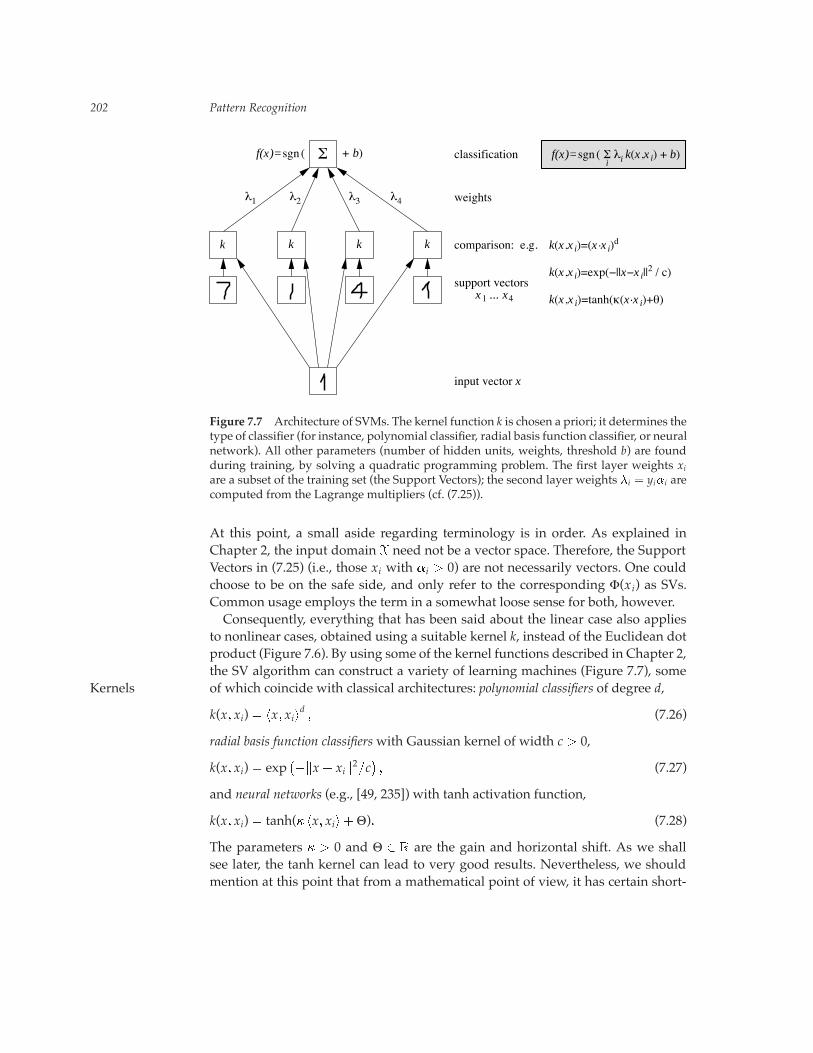
Figure 7.7 Architecture of SVMs. The kernel function k is chosen a priori; it determines thetype of classifier (for instance, polynomial classifier, radial basis function classifier, or neuralnetwork). All other parameters (number of hidden units, weights, threshold b) are foundduring training, by solving a quadratic programming problem. The first layer weights xiare a subset of the training set (the Support Vectors); the second layer weights �i � yi�i arecomputed from the Lagrange multipliers (cf. (7.25)).
At this point, a small aside regarding terminology is in order. As explained inChapter 2, the input domain � need not be a vector space. Therefore, the SupportVectors in (7.25) (i.e., those xi with �i � 0) are not necessarily vectors. One couldchoose to be on the safe side, and only refer to the corresponding Φ(xi) as SVs.Common usage employs the term in a somewhat loose sense for both, however.Consequently, everything that has been said about the linear case also applies
to nonlinear cases, obtained using a suitable kernel k, instead of the Euclidean dotproduct (Figure 7.6). By using some of the kernel functions described in Chapter 2,the SV algorithm can construct a variety of learning machines (Figure 7.7), someof which coincide with classical architectures: polynomial classifiers of degree d,Kernels
k(x� xi) � �x� xi�d � (7.26)
radial basis function classifierswith Gaussian kernel of width c � 0,
k(x� xi) � exp��x� xi2�c
�� (7.27)
and neural networks (e.g., [49, 235]) with tanh activation function,
k(x� xi) � tanh(� �x� xi��Θ)� (7.28)
The parameters � � 0 and Θ � � are the gain and horizontal shift. As we shallsee later, the tanh kernel can lead to very good results. Nevertheless, we shouldmention at this point that from a mathematical point of view, it has certain short-
7.4 Nonlinear Support Vector Classifiers 203
comings, cf. the discussion following (2.69).To find the decision function (7.25), we solve the following problem (cf. (7.17)):Quadratic
Programmaximize
�
W(�) �m
∑i�1
�i �12
m
∑i� j�1
�i� j yiy jk(xi� xj)� (7.29)
subject to the constraints (7.18) and (7.19).If k is positive definite, Qij :� (yiyjk(xi� xj))i j is a positive definite matrix (Prob-
lem 7.6), which provides us with a convex problem that can be solved efficiently(cf. Chapter 6). To see this, note that (cf. Proposition 2.16)
m
∑i� j�1
�i� jyi y jk(xi� xj) �
m
∑i�1
�i yiΦ(xi)�m
∑j�1
� j y jΦ(xj)
� 0� (7.30)
for all � � �m .
As described in Chapter 2, we can actually use a larger class of kernels withoutdestroying the convexity of the quadratic program. This is due to the fact thatthe constraint (7.19) excludes certain parts of the space of multipliers �i. As aresult, we only need the kernel to be positive definite on the remaining points.This is precisely guaranteed if we require k to be conditionally positive definite(see Definition 2.21). In this case, we have ��Q� � 0 for all coefficient vectors �satisfying (7.19).To compute the threshold b, we take into account that due to the KKT conditionsThreshold
(7.16), � j � 0 implies (using (7.24))m
∑i�1yi�ik(xj� xi)� b � yj� (7.31)
Thus, the threshold can for instance be obtained by averaging
b � yj �m
∑i�1yi�ik(xj� xi)� (7.32)
over all points with � j � 0; in other words, all SVs. Alternatively, one can computeb from the value of the corresponding double dual variable; see Section 10.3 fordetails. Sometimes it is also useful not to use the “optimal” b, but to change it inorder to adjust the number of false positives and false negatives.Figure 1.7 shows how a simple binary toy problem is solved, using a Support
Vector Machine with a radial basis function kernel (7.27). Note that the SVs are thepatterns closest to the decision boundary — not only in the feature space, whereby construction, the SVs are the patterns closest to the separating hyperplane, butalso in the input space depicted in the figure. This feature differentiates SVMsfrom other types of classifiers. Figure 7.8 shows both the SVs and the centers ex-tracted by k-means, which are the expansion patterns that a classical RBF networkapproach would employ.In a study comparing the two approaches on the USPS problem of handwrittenComparison to
RBF Network character recognition, a SVM with a Gaussian kernel outperformed the classicalRBF network using Gaussian kernels [482]. A hybrid approach, where the SVM
204 Pattern Recognition
✕
✕
✕
✕
✕
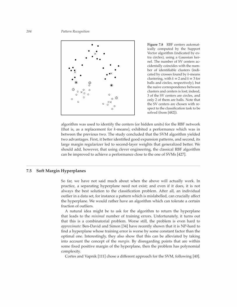
Figure 7.8 RBF centers automat-ically computed by the SupportVector algorithm (indicated by ex-tra circles), using a Gaussian ker-nel. The number of SV centers ac-cidentally coincides with the num-ber of identifiable clusters (indi-cated by crosses found by k-meansclustering, with k � 2 and k� 3 forballs and circles, respectively), butthe naive correspondence betweenclusters and centers is lost; indeed,3 of the SV centers are circles, andonly 2 of them are balls. Note thatthe SV centers are chosen with re-spect to the classification task to besolved (from [482]).
algorithm was used to identify the centers (or hidden units) for the RBF network(that is, as a replacement for k-means), exhibited a performance which was inbetween the previous two. The study concluded that the SVM algorithm yieldedtwo advantages. First, it better identified good expansion patterns, and second, itslarge margin regularizer led to second-layer weights that generalized better. Weshould add, however, that using clever engineering, the classical RBF algorithmcan be improved to achieve a performance close to the one of SVMs [427].
7.5 Soft Margin Hyperplanes
So far, we have not said much about when the above will actually work. Inpractice, a separating hyperplane need not exist; and even if it does, it is notalways the best solution to the classification problem. After all, an individualoutlier in a data set, for instance a pattern which is mislabelled, can crucially affectthe hyperplane. We would rather have an algorithm which can tolerate a certainfraction of outliers.A natural idea might be to ask for the algorithm to return the hyperplane
that leads to the minimal number of training errors. Unfortunately, it turns outthat this is a combinatorial problem. Worse still, the problem is even hard toapproximate: Ben-David and Simon [34] have recently shown that it is NP-hard tofind a hyperplane whose training error is worse by some constant factor than theoptimal one. Interestingly, they also show that this can be alleviated by takinginto account the concept of the margin. By disregarding points that are withinsome fixed positive margin of the hyperplane, then the problem has polynomialcomplexity.Cortes and Vapnik [111] chose a different approach for the SVM, following [40].
7.5 Soft Margin Hyperplanes 205
To allow for the possibility of examples violating (7.11), they introduced so-calledslack variables,Slack Variables
�i � 0� where i � 1� � � � �m� (7.33)
and use relaxed separation constraints (cf. (7.11)),
yi(�xi�w�� b) � 1� �i� i � 1� � � � �m� (7.34)
Clearly, by making �i large enough, the constraint on (xi� yi) can always be met. Inorder not to obtain the trivial solution where all �i take on large values, we thusneed to penalize them in the objective function. To this end, a term ∑i �i is includedin (7.10).In the simplest case, referred to as the C-SV classifier, this is done by solving, forC-SVC
some C � 0,
minimizew������m
� (w� �) �12�w�2 �
Cm
m
∑i�1
�i� (7.35)
subject to the constraints (7.33) and (7.34). It is instructive to compare this toTheorem 7.3, considering the case � � 1. Whenever the constraint (7.34) is metwith �i � 0, the corresponding point will not be a margin error. All non-zero slacks� correspond to margin errors; hence, roughly speaking, the fraction of marginerrors in Theorem 7.3 increases with the second term in (7.35). The capacity term,on the other hand, increases with �w�. Hence, for a suitable positive constant C,this approach approximately minimizes the right hand side of the bound.Note, however, that if many of the �i attain large values (in other words, if the
classes to be separated strongly overlap, for instance due to noise), then ∑mi�1 �i canbe significantly larger than the fraction of margin errors. In that case, there is noguarantee that the hyperplane will generalize well.As in the separable case (7.15), the solution can be shown to have an expansion
w �m
∑i�1
�i yixi� (7.36)
where non-zero coefficients �i can only occur if the corresponding example (xi� yi)precisely meets the constraint (7.34). Again, the problem only depends on dotproducts in�, which can be computed by means of the kernel.The coefficients �i are found by solving the following quadratic programming
problem:
maximize���m
W(�) �m
∑i�1
�i �12
m
∑i� j�1
�i� j yiy jk(xi� xj)� (7.37)
subject to 0 � �i �Cmfor all i � 1� � � � �m� (7.38)
andm
∑i�1
�i yi � 0� (7.39)
To compute the threshold b, we take into account that due to (7.34), for Support
206 Pattern Recognition
Vectors xj for which � j � 0, we have (7.31). Thus, the threshold can be obtained byaveraging (7.32) over all Support Vectors x j (recall that they satisfy � j � 0) with� j � C.In the above formulation, C is a constant determining the trade-off between
two conflicting goals: minimizing the training error, and maximizing the margin.Unfortunately, C is a rather unintuitive parameter, and we have no a priori wayto select it.9 Therefore, a modification was proposed in [481], which replaces C bya parameter ; the latter will turn out to control the number of margin errors and-SVCSupport Vectors.As a primal problem for this approach, termed the -SV classifier, we consider
minimizew������m ���b��
� (w� �� �) �12�w�2 � ��
1m
m
∑i�1
�i (7.40)
subject to yi(�xi�w�� b) � �� �i (7.41)
and �i � 0� � � 0� (7.42)
Note that no constant C appears in this formulation; instead, there is a parameter , and also an additional variable � to be optimized. To understand the role of�, note that for � � 0, the constraint (7.41) simply states that the two classes areseparated by the margin 2��w� (cf. Problem 7.4).To explain the significance of , let us first recall the term margin error: by this,Margin Error
we denote points with �i � 0. These are points which are either errors, or lie withinthe margin. Formally, the fraction of margin errors is
R�
emp[g] :�1m��i�yig(xi) � �� � (7.43)
Here, g is used to denote the argument of the sgn in the decision function (7.25):f � sgn Æg. We are now in a position to state a result that explains the significanceof .-Property
Proposition 7.5 ([481]) Suppose we run -SVC with k on some data with the result that� � 0. Then
(i) is an upper bound on the fraction of margin errors.
(ii) is a lower bound on the fraction of SVs.
(iii) Suppose the data (x1� y1)� � � � � (xm� ym) were generated iid from a distributionP(x� y) � P(x)P(y�x), such that neither P(x� y � 1) nor P(x� y � �1) contains any dis-crete component. Suppose, moreover, that the kernel used is analytic and non-constant.With probability 1, asymptotically, equals both the fraction of SVs and the fraction oferrors.
The proof can be found in Section A.2.Before we get into the technical details of the dual derivation, let us take a look
9. As a default value, we use C�m � 10 unless stated otherwise.
7.5 Soft Margin Hyperplanes 207
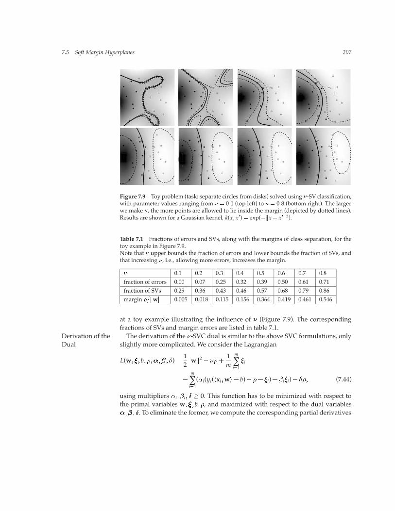
Figure 7.9 Toy problem (task: separate circles from disks) solved using �-SV classification,with parameter values ranging from � � 0�1 (top left) to � � 0�8 (bottom right). The largerwe make �, the more points are allowed to lie inside the margin (depicted by dotted lines).Results are shown for a Gaussian kernel, k(x� x�) � exp(��x� x��2).
Table 7.1 Fractions of errors and SVs, along with the margins of class separation, for thetoy example in Figure 7.9.Note that � upper bounds the fraction of errors and lower bounds the fraction of SVs, andthat increasing �, i.e., allowing more errors, increases the margin.
� 0.1 0.2 0.3 0.4 0.5 0.6 0.7 0.8fraction of errors 0.00 0.07 0.25 0.32 0.39 0.50 0.61 0.71fraction of SVs 0.29 0.36 0.43 0.46 0.57 0.68 0.79 0.86margin ���w� 0.005 0.018 0.115 0.156 0.364 0.419 0.461 0.546
at a toy example illustrating the influence of (Figure 7.9). The correspondingfractions of SVs and margin errors are listed in table 7.1.The derivation of the -SVC dual is similar to the above SVC formulations, onlyDerivation of the
Dual slightly more complicated. We consider the Lagrangian
L(w� �� b� ������ Æ)�12�w�2 � ��
1m
m
∑i�1
�i
�m
∑i�1(�i(yi(�xi�w�� b)� �� �i)� �i�i)� Æ�� (7.44)
using multipliers �i� �i� Æ � 0. This function has to be minimized with respect tothe primal variables w� �� b� �, and maximized with respect to the dual variables���� Æ. To eliminate the former, we compute the corresponding partial derivatives
208 Pattern Recognition
and set them to 0, obtaining the following conditions:
w �m
∑i�1
�i yixi� (7.45)
�i � �i � 1m� (7.46)m
∑i�1
�i yi � 0� (7.47)
m
∑i�1
�i � Æ � � (7.48)
Again, in the SV expansion (7.45), the �i that are non-zero correspond to a con-straint (7.41) which is precisely met.Substituting (7.45) and (7.46) into L, using �i� �i� Æ � 0, and incorporating ker-
nels for dot products, leaves us with the following quadratic optimization problemfor -SV classification:Quadratic
Programfor -SVC maximize
���mW(�) � �
12
m
∑i� j�1
�i� j yi y jk(xi� xj)� (7.49)
subject to 0 � �i �1m� (7.50)
m
∑i�1
�i yi � 0� (7.51)
m
∑i�1
�i � � (7.52)
As above, the resulting decision function can be shown to take the form
f (x) � sgn
�m
∑i�1
�i yik(x� xi)� b
�� (7.53)
Compared with the C-SVC dual (7.37), there are two differences. First, there is anadditional constraint (7.52).10 Second, the linear term ∑mi�1 �i no longer appears inthe objective function (7.49). This has an interesting consequence: (7.49) is nowquadratically homogeneous in �. It is straightforward to verify that the samedecision function is obtained if we start with the primal function
� (w� �� �)�12�w�2 �C
����
1m
m
∑i�1
�i
�� (7.54)
10. The additional constraint makes it more challenging to come up with efficient trainingalgorithms for large datasets. So far, two approaches have been proposed which work well.One of them slightly modifies the primal problem in order to avoid the other equality con-straint (related to the offset b) [98]. The other one is a direct generalization of a correspond-ing algorithm for C-SVC, which reduces the problem for each chunk to a linear system, andwhich does not suffer any disadvantages from the additional constraint [407, 408]. See alsoSections 10.3.2, 10.4.3, and 10.6.3 for further details.
7.5 Soft Margin Hyperplanes 209
i.e., if one does use C, cf. Problem 7.16.To compute the threshold b and the margin parameter �, we consider two
sets S�, of identical size s � 0, containing SVs xi with 0 � �i � 1 and yi � 1,respectively. Then, due to the KKT conditions, (7.41) becomes an equality with�i � 0. Hence, in terms of kernels,
b � �12s ∑
x�S��S�
m
∑j�1
� j y jk(x� xj)� (7.55)
� �12s
�∑x�S�
m
∑j�1
� j y jk(x� xj)� ∑x�S
�
m
∑j�1
� j y jk(x� xj)�� (7.56)
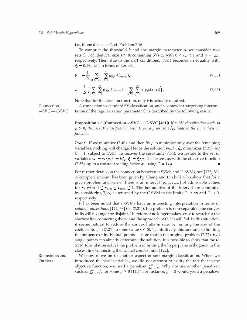
Note that for the decision function, only b is actually required.A connection to standard SV classification, and a somewhat surprising interpre-Connection
-SVC — C-SVC tation of the regularization parameter C, is described by the following result:
Proposition 7.6 (Connection -SVC— C-SVC [481]) If -SV classification leads to� � 0, then C-SV classification, with C set a priori to 1�, leads to the same decisionfunction.
Proof If we minimize (7.40), and then fix � to minimize only over the remainingvariables, nothing will change. Hence the solution w0� b0� �0 minimizes (7.35), forC � 1, subject to (7.41). To recover the constraint (7.34), we rescale to the set ofvariables w�
� w�� b� � b�� �� � ��. This leaves us with the objective function(7.35), up to a constant scaling factor �2, using C � 1�.
For further details on the connection between -SVMs and C-SVMs, see [122, 38].A complete account has been given by Chang and Lin [98], who show that for agiven problem and kernel, there is an interval [min� max] of admissible valuesfor , with 0 � min � max � 1. The boundaries of the interval are computedby considering ∑i �i as returned by the C-SVM in the limits C�� and C� 0,respectively.It has been noted that -SVMs have an interesting interpretation in terms of
reduced convex hulls [122, 38] (cf. (7.21)). If a problem is non-separable, the convexhulls will no longer be disjoint. Therefore, it no longermakes sense to search for theshortest line connecting them, and the approach of (7.22) will fail. In this situation,it seems natural to reduce the convex hulls in size, by limiting the size of thecoefficients ci in (7.21) to some value (0� 1). Intuitively, this amounts to limitingthe influence of individual points — note that in the original problem (7.22), twosingle points can already determine the solution. It is possible to show that the -SVM formulation solves the problem of finding the hyperplane orthogonal to theclosest line connecting the reduced convex hulls [122].We now move on to another aspect of soft margin classification. When weRobustness and
Outliers introduced the slack variables, we did not attempt to justify the fact that in theobjective function, we used a penalizer ∑mi�1 �i. Why not use another penalizer,such as ∑mi�1 �
pi , for some p � 0 [111]? For instance, p � 0 would yield a penalizer
210 Pattern Recognition
that exactly counts the number of margin errors. Unfortunately, however, it is also apenalizer that leads to a combinatorial optimization problem. Penalizers yieldingoptimization problems that are particularly convenient, on the other hand, areobtained for p � 1 and p � 2. By default, we use the former, as it possesses anadditional property which is statistically attractive. As the following propositionshows, linearity of the target function in the slack variables �i leads to a certain“outlier” resistance of the estimator. As above, we use the shorthand xi for Φ(xi).
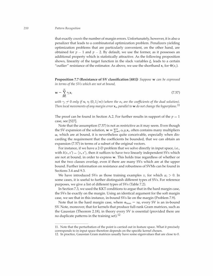
Proposition 7.7 (Resistance of SV classification [481]) Suppose w can be expressedin terms of the SVs which are not at bound,
w �m
∑i�1
�ixi (7.57)
with �i �� 0 only if �i (0� 1m) (where the �i are the coefficients of the dual solution).Then local movements of any margin error xm parallel tow do not change the hyperplane.11
The proof can be found in Section A.2. For further results in support of the p � 1case, see [527].Note that the assumption (7.57) is not as restrictive as it may seem. Even though
the SV expansion of the solution,w� ∑mi�1 �i yixi, often contains many multipliers�i which are at bound, it is nevertheless quite conceivable, especially when dis-carding the requirement that the coefficients be bounded, that we can obtain anexpansion (7.57) in terms of a subset of the original vectors.For instance, if we have a 2-D problem that we solve directly in input space, i.e.,
with k(x� x�) � �x� x��, then it suffices to have two linearly independent SVs whichare not at bound, in order to express w. This holds true regardless of whether ornot the two classes overlap, even if there are many SVs which are at the upperbound. Further information on resistance and robustness of SVMs can be found inSections 3.4 and 9.3.We have introduced SVs as those training examples xi for which �i � 0. In
some cases, it is useful to further distinguish different types of SVs. For referencepurposes, we give a list of different types of SVs (Table 7.2).In Section 7.3, we used the KKT conditions to argue that in the hardmargin case,
the SVs lie exactly on the margin. Using an identical argument for the soft margincase, we see that in this instance, in-bound SVs lie on the margin (Problem 7.9).Note that in the hard margin case, where �max ��, every SV is an in-bound
SV. Note, moreover, that for kernels that produce full-rank Grammatrices, such asthe Gaussian (Theorem 2.18), in theory every SV is essential (provided there areno duplicate patterns in the training set).12
11. Note that the perturbation of the point is carried out in feature space. What it preciselycorresponds to in input space therefore depends on the specific kernel chosen.12. In practice, Gaussian Gram matrices usually have some eigenvalues that are close to 0.

7.6 Multi-Class Classification 211
Table 7.2 Overview of different types of SVs. In each case, the condition on the Lagrangemultipliers �i (corresponding to an SV xi) is given. In the table, �max stands for the upperbound in the optimization problem; for instance, �max � C
m in (7.38) and �max �1m in (7.50).
Type of SV Definition Properties(standard) SV 0 � �i lies on or in marginin-bound SV 0 � �i � �max lies on marginbound SV �i � �max usually lies in margin
(“margin error”)essential SV appears in all possible becomes margin error
expansions of solution when left out (Section 7.3)
7.6 Multi-Class Classification
So far, we have talked about binary classification, where the class labels canonly take two values: 1. Many real-world problems, however, have more thantwo classes — an example being the widely studied optical character recognition(OCR) problem. We will now review some methods for dealing with this issue.
7.6.1 One Versus the Rest
To get M-class classifiers, it is common to construct a set of binary classifiersf 1� � � � � f M, each trained to separate one class from the rest, and combine themby doing the multi-class classification according to the maximal output before ap-plying the sgn function; that is, by taking
argmaxj�1�����M
gj(x)� where gj(x) �m
∑i�1yi�
ji k(x� xi)� b
j (7.58)
(note that f j(x) � sgn (gj(x)), cf. (7.25)).The values gj(x) can also be used for reject decisions. To see this, we considerReject Decisions
the difference between the two largest g j(x) as a measure of confidence in theclassification of x. If that measure falls short of a threshold , the classifier rejectsthe pattern and does not assign it to a class (it might instead be passed on toa human expert). This has the consequence that on the remaining patterns, alower error rate can be achieved. Some benchmark comparisons report a quantityreferred to as the punt error, which denotes the fraction of test patterns that mustbe rejected in order to achieve a certain accuracy (say 1% error) on the remainingtest samples. To compute it, the value of is adjusted on the test set [64].The main shortcoming of (7.58), sometimes called the winner-takes-all approach,
is that it is somewhat heuristic. The binary classifiers used are obtained by trainingon different binary classification problems, and thus it is unclear whether their
212 Pattern Recognition
real-valued outputs (before thresholding) are on comparable scales.13 This can bea problem, since situations often arise where several binary classifiers assign thepattern to their respective class (or where none does); in this case, one class mustbe chosen by comparing the real-valued outputs.In addition, binary one-versus-the-rest classifiers have been criticized for deal-
ing with rather asymmetric problems. For instance, in digit recognition, the clas-sifier trained to recognize class ‘7’ is usually trained on many more negative thanpositive examples. We can deal with these asymmetries by using values of the reg-ularization constant C which differ for the respective classes (see Problem 7.10). Ithas nonetheless been argued that the following approach, which is more symmet-ric from the outset, can be advantageous.
7.6.2 Pairwise Classification
In pairwise classification, we train a classifier for each possible pair of classes[178, 463, 233, 311]. For M classes, this results in (M � 1)M�2 binary classifiers.This number is usually larger than the number of one-versus-the-rest classifiers;for instance, if M � 10, we need to train 45 binary classifiers rather than 10 asin the method above. Although this suggests large training times, the individualproblems that we need to train on are significantly smaller, and if the trainingalgorithm scales superlinearly with the training set size, it is actually possible tosave time.Similar considerations apply to the runtime execution speed. When we try to
classify a test pattern, we evaluate all 45 binary classifiers, and classify accordingto which of the classes gets the highest number of votes. A vote for a givenclass is defined as a classifier putting the pattern into that class.14 The individualclassifiers, however, are usually smaller in size (they have fewer SVs) than theywould be in the one-versus-the-rest approach. This is for two reasons: First, thetraining sets are smaller, and second, the problems to be learned are usually easier,since the classes have less overlap.Nevertheless, if M is large, and we evaluate the (M� 1)M�2 classifiers, then the
resulting system may be slower than the corresponding one-versus-the-rest SVM.To illustrate this weakness, consider the following hypothetical situation: Suppose,in a digit recognition task, that after evaluating the first few binary classifiers,both digit 7 and digit 8 seem extremely unlikely (they already “lost” on severalclassifiers). In that case, it would seem pointless to evaluate the 7-vs-8 classifier.This idea can be cast into a precise framework by embedding the binary classifiersinto a directed acyclic graph. Each classification run then corresponds to a directedtraversal of that graph, and classification can be much faster [411].
13. Note, however, that some effort has gone into developing methods for transforming thereal-valued outputs into class probabilities [521, 486, 410].14. Some care has to be exercised in tie-breaking. For further detail, see [311].
7.6 Multi-Class Classification 213
7.6.3 Error-Correcting Output Coding
The method of error-correcting output codes was developed in [142], and lateradapted to the case of SVMs [5]. In a nutshell, the idea is as follows. Just as wecan generate a binary problem from a multiclass problem by separating one classfrom the rest — digit 0 from digits 1 through 9, say — we can generate a largenumber of further binary problems by splitting the original set of classes into twosubsets. For instance, we could separate the even digits from the odd ones, or wecould separate digits 0 through 4 from 5 through 9. It is clear that if we designa set of binary classifiers f 1� � � � � f L in the right way, then the binary responseswill completely determine the class of a test patterns. Each class corresponds to aunique vector in ��1�L; for M classes, we thus get a so-called decoding matrix M ���1�M�L. What happens if the binary responses are inconsistent with each other;if, for instance, the problem is noisy, or the training sample is too small to estimatethe binary classifiers reliably? Formally, this means that we will obtain a vectorof responses f 1(x)� � � � � f L(x) which does not occur in the matrix M. To deal withthese cases, [142] proposed designing a clever set of binary problems, which yieldsrobustness against some errors. Here, the closest match between the vector ofresponses and the rows of the matrix is determined using the Hamming distance(the number of entries where the two vectors differ; essentially, the L� distance).Now imagine a situation where the code is such that the minimal Hammingdistance is three. In this case, we can guarantee that we will correctly classify alltest examples which lead to at most one error amongst the binary classifiers.This method produces very good results in multi-class tasks; nevertheless, it
has been pointed out that it does not make use of a crucial quantity in classifiers:the margin. Recently [5], a version was developed that replaces the Hamming-based decoding with a more sophisticated scheme that takes margins into account.Recommendations are also made regarding how to design good codes for marginclassifiers, such as SVMs.
7.6.4 Multi-Class Objective Functions
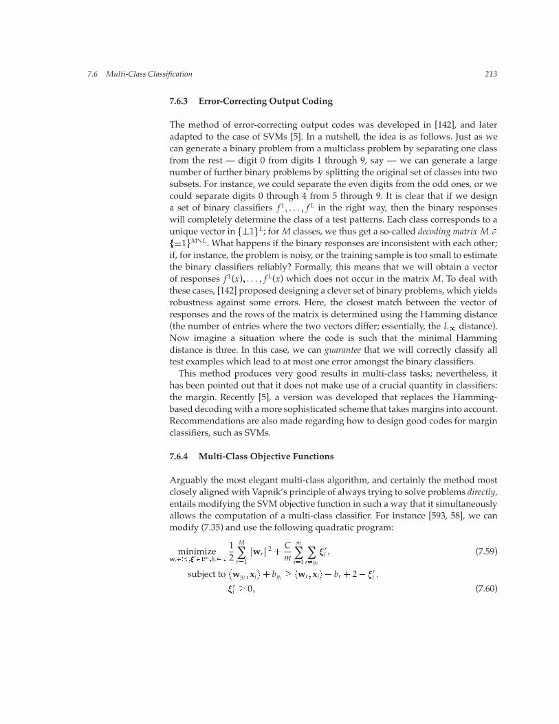
Arguably the most elegant multi-class algorithm, and certainly the method mostclosely aligned with Vapnik’s principle of always trying to solve problems directly,entails modifying the SVM objective function in such a way that it simultaneouslyallows the computation of a multi-class classifier. For instance [593, 58], we canmodify (7.35) and use the following quadratic program:
minimizewr����r��m �br��
12
M
∑r�1
�wr�2 �Cm
m
∑i�1
∑r ��yi
�ri � (7.59)
subject to�wyi � xi
�� byi � �wr� xi� br � 2� �ri �
�ri � 0� (7.60)
214 Pattern Recognition
where m � �1� � � � �M� yi, and yi � �1� � � � �M� is the multi-class label of thepattern xi (cf. Problem 7.17).In terms of accuracy, the results obtained with this approach are comparable to
those obtained with the widely used one-versus-the-rest approach. Unfortunately,the optimization problem is such that it has to deal with all SVs at the sametime. In the other approaches, the individual binary classifiers usually have muchsmaller SV sets, with beneficial effects on the training time. For further multiclassapproaches, see [160, 323]. Generalizations to multi-label problems, where patternsare allowed to belong to several classes at the same time, are discussed in [162].Overall, it is fair to say that there is probably no multi-class approach that gen-
erally outperforms the others. For practical problems, the choice of approach willdepend on constraints at hand. Relevant factors include the required accuracy, thetime available for development and training, and the nature of the classificationproblem (e.g., for a problem with very many classes, it would not be wise to use(7.59)). That said, a simple one-against-the-rest approach often produces accept-able results.
7.7 Variations on a Theme
There are a number of variations of the standard SV classification algorithm, suchas the elegant leave-one-out machine [589, 592] (see also Section 12.2.2 below), theidea of Bayes point machines [451, 239, 453, 545, 392], and extensions to featureselection [70, 224, 590]. Due to lack of space, we only describe one of the variations;namely, linear programming machines.Linear
ProgrammingMachines
As we have seen above, the SVM approach automatically leads to a decisionfunction of the form (7.25). Let us rewrite it as f (x)� sgn (g(x)), with
g(x) �m
∑i�1
�ik(x� xi)� b� (7.61)
In Chapter 4, we showed that this form of the solution is essentially a consequenceof the form of the regularizer �w�2 (Theorem 4.2). The idea of linear programming(LP) machines is to use the kernel expansion as an ansatz for the solution, but touse a different regularizer, namely the �1 norm of the coefficient vector [343, 344,�1 Regularizer74, 184, 352, 37, 591, 593, 39]. The main motivation for this is that this regularizeris known to induce sparse expansions (see Chapter 4).This amounts to the objective function
Rreg[g] :�1m���1 �C Remp[g]� (7.62)
where ���1 � ∑mi�1 ��i� denotes the �1 norm in coefficient space, using the softmargin empirical risk,
Remp[g] �1m∑i
�i� (7.63)
7.8 Experiments 215
with slack terms
�i �max�1� yig(xi)� 0�� (7.64)
We thus obtain a linear programming problem;
minimize�����m �b��
1m
m∑i�1(�i ���
i )�Cm∑i�1
�i�
subject to yig(xi) � 1� �i�
�i� ��
i � �i � 0�
(7.65)
Here, we have dealt with the �1-norm by splitting each component �i into itspositive and negative part: �i � �i � ��
i in (7.61). The solution differs from (7.25)in that it is no longer necessarily the case that each expansion pattern has a weight�i yi, whose sign equals its class label. This property would have to be enforcedseparately (Problem 7.19). Moreover, it is also no longer the case that the expansionpatterns lie on or beyond the margin — in LP machines, they can basically beanywhere.LP machines can also benefit from the �-trick. In this case, the programming�-LPMs
problem can be shown to take the following form [212]:
minimize�����m �b����
1m
m∑i�1
�i � ���
subject to 1m
m∑i�1(�i � ��
i ) � 1�
yig(xi) � �� �i�
�i� ��
i � �i� � � 0�
(7.66)
We will not go into further detail at this point. Additional information onlinear programming machines from a regularization point of view is given inSection 4.9.2.
7.8 Experiments
7.8.1 Digit Recognition Using Different Kernels
Handwritten digit recognition has long served as a test bed for evaluating andbenchmarking classifiers [318, 64, 319]. Thus, it was imperative in the early days ofSVM research to evaluate the SVmethod onwidely used digit recognition tasks. Inthis section we report results on the US Postal Service (USPS) database (describedin Section A.1). We shall return to the character recognition problem in Chapter 11,where we consider the larger MNIST database.As described above, the difference between C-SVC and �-SVC lies only in the
fact that we have to select a different parameter a priori. If we are able to do this
216 Pattern Recognition
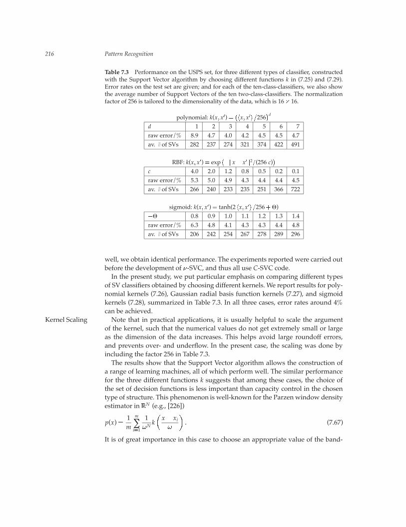
Table 7.3 Performance on the USPS set, for three different types of classifier, constructedwith the Support Vector algorithm by choosing different functions k in (7.25) and (7.29).Error rates on the test set are given; and for each of the ten-class-classifiers, we also showthe average number of Support Vectors of the ten two-class-classifiers. The normalizationfactor of 256 is tailored to the dimensionality of the data, which is 16� 16.
polynomial: k(x� x�) ���x� x���256
�d
d 1 2 3 4 5 6 7raw error/% 8.9 4.7 4.0 4.2 4.5 4.5 4.7av. # of SVs 282 237 274 321 374 422 491
RBF: k(x� x�) � exp���x� x��2�(256 c)
�
c 4.0 2.0 1.2 0.8 0.5 0.2 0.1raw error/% 5.3 5.0 4.9 4.3 4.4 4.4 4.5av. # of SVs 266 240 233 235 251 366 722
sigmoid: k(x� x�) � tanh(2 �x� x���256�Θ)�Θ 0.8 0.9 1.0 1.1 1.2 1.3 1.4raw error/% 6.3 4.8 4.1 4.3 4.3 4.4 4.8av. # of SVs 206 242 254 267 278 289 296
well, we obtain identical performance. The experiments reported were carried outbefore the development of �-SVC, and thus all use C-SVC code.In the present study, we put particular emphasis on comparing different types
of SV classifiers obtained by choosing different kernels. We report results for poly-nomial kernels (7.26), Gaussian radial basis function kernels (7.27), and sigmoidkernels (7.28), summarized in Table 7.3. In all three cases, error rates around 4%can be achieved.Note that in practical applications, it is usually helpful to scale the argumentKernel Scaling
of the kernel, such that the numerical values do not get extremely small or largeas the dimension of the data increases. This helps avoid large roundoff errors,and prevents over- and underflow. In the present case, the scaling was done byincluding the factor 256 in Table 7.3.The results show that the Support Vector algorithm allows the construction of
a range of learning machines, all of which perform well. The similar performancefor the three different functions k suggests that among these cases, the choice ofthe set of decision functions is less important than capacity control in the chosentype of structure. This phenomenon is well-known for the Parzen window densityestimator in � N (e.g., [226])
p(x) �1m
m
∑i�1
1Nk�x� xi
�� (7.67)
It is of great importance in this case to choose an appropriate value of the band-
7.8 Experiments 217
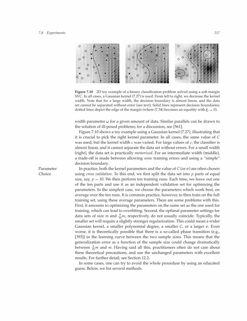
Figure 7.10 2D toy example of a binary classification problem solved using a soft marginSVC. In all cases, a Gaussian kernel (7.27) is used. From left to right, we decrease the kernelwidth. Note that for a large width, the decision boundary is almost linear, and the dataset cannot be separated without error (see text). Solid lines represent decision boundaries;dotted lines depict the edge of the margin (where (7.34) becomes an equality with �i � 0).
width parameter for a given amount of data. Similar parallels can be drawn tothe solution of ill-posed problems; for a discussion, see [561].Figure 7.10 shows a toy example using a Gaussian kernel (7.27), illustrating that
it is crucial to pick the right kernel parameter. In all cases, the same value of Cwas used, but the kernel width c was varied. For large values of c, the classifier isalmost linear, and it cannot separate the data set without errors. For a small width(right), the data set is practically memorized. For an intermediate width (middle),a trade-off is made between allowing some training errors and using a “simple”decision boundary.In practice, both the kernel parameters and the value of C (or �) are often chosenParameter
Choice using cross validation. To this end, we first split the data set into p parts of equalsize, say, p � 10. We then perform ten training runs. Each time, we leave out oneof the ten parts and use it as an independent validation set for optimizing theparameters. In the simplest case, we choose the parameters which work best, onaverage over the ten runs. It is common practice, however, to then train on the fulltraining set, using these average parameters. There are some problems with this.First, it amounts to optimizing the parameters on the same set as the one used fortraining, which can lead to overfitting. Second, the optimal parameter settings fordata sets of size m and 9
10m, respectively, do not usually coincide. Typically, thesmaller set will require a slightly stronger regularization. This could mean a widerGaussian kernel, a smaller polynomial degree, a smaller C, or a larger � . Evenworse, it is theoretically possible that there is a so-called phase transition (e.g.,[393]) in the learning curve between the two sample sizes. This means that thegeneralization error as a function of the sample size could change dramaticallybetween 9
10m and m. Having said all this, practitioners often do not care aboutthese theoretical precautions, and use the unchanged parameters with excellentresults. For further detail, see Section 12.2.In some cases, one can try to avoid the whole procedure by using an educated
guess. Below, we list several methods.
218 Pattern Recognition
Use parameter settings that have worked well for similar problems. Here, somecare has to be exercised in the scaling of kernel parameters. For instance, whenusing an RBF kernel, cmust be rescaled to ensure that �xi � xj�2c roughly lies inthe same range, even if the scaling and dimension of the data are different.
For many problems, there is some prior expectation regarding the typical errorrate. Let us assume we are looking at an image classification task, and we havealready tried three other approaches, all of which yielded around 5% test error.Using ��SV classifiers, we can incorporate this knowledge by choosing a valuefor � which is in that range, say � � 5%. The reason for this guess is that we know(Proposition 7.5) that the margin error is then below 5%, which in turn implies thatthe training error is below 5%. The training error will typically be smaller than thetest error, thus it is consistent that it should be upper bounded by the 5% test error.
In a slightly less elegant way, one can try to mimic this procedure for C-SVclassifiers. To this end, we start off with a large value of C, and reduce it untilthe number of Lagrange multipliers that are at the upper bound (in other words,the number of margin errors) is in a suitable range (say, somewhat below 5%).Compared to the above procedure for choosing � , the disadvantage is that thisentails a number of training runs. We can also monitor the number of actualtraining errors during the training runs, but since not every margin error is atraining error, this is often less sensitive. Indeed, the difference between trainingerror and test error can often be quite substantial. For instance, on the USPS set,most of the results reported here were obtained with systems that had essentiallyzero training error.
One can put forward scaling arguments which indicate that C � 1R2, where Ris a measure for the range of the data in feature space that scales like the lengthof the points in �. Examples thereof are the standard deviation of the distance ofthe points to their mean, the radius of the smallest sphere containing the data (cf.(5.61) and (8.17)), or, in some cases, the maximum (or mean) length k(xi� xi) overall data points (see Problem 7.25).
Finally, we can use theoretical tools such as VC bounds (see, for instance, Fig-ure 5.5) or leave-one-out bounds (Section 12.2).
Having seen that different types of SVCs lead to similar performance, the ques-tion arises as to how these performances compare with other approaches. Table 7.4gives a summary of a number of results on the USPS set. Note that the best SVMresult is 3�0%; it uses additional techniques that we shall explain in chapters 11and 13. It is known that the USPS test set is rather difficult — the human error rateis 2.5% [79]. For a discussion, see [496]. Note, moreover, that some of the resultsreported in the literature for the USPS set were obtained with an enhanced train-ing set: For instance, the study of Drucker et al. [148] used an enlarged training setof size 9709, containing some additional machine-printed digits, and found thatthis improves the accuracy on the test set. Similarly, Bottou and Vapnik [65] useda training set of size 9840. Since there are no machine-printed digits in the com-
7.8 Experiments 219
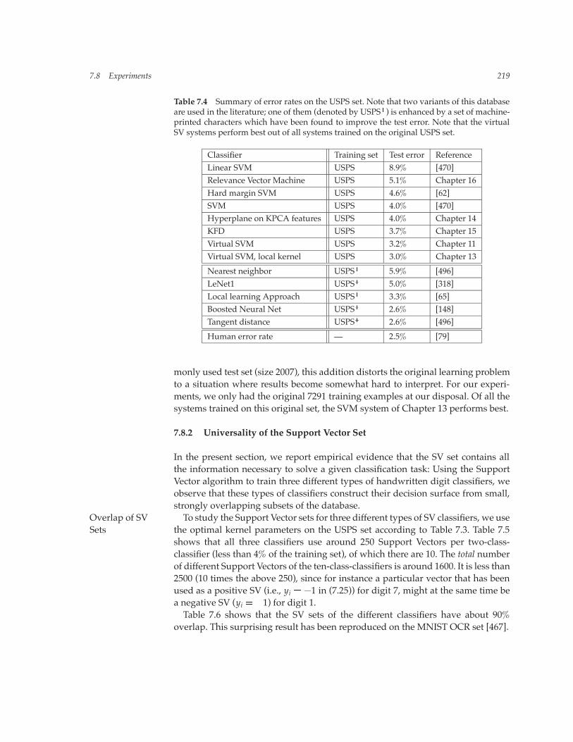
Table 7.4 Summary of error rates on the USPS set. Note that two variants of this databaseare used in the literature; one of them (denoted by USPS�) is enhanced by a set of machine-printed characters which have been found to improve the test error. Note that the virtualSV systems perform best out of all systems trained on the original USPS set.
Classifier Training set Test error ReferenceLinear SVM USPS 8.9% [470]Relevance Vector Machine USPS 5.1% Chapter 16Hard margin SVM USPS 4.6% [62]SVM USPS 4.0% [470]Hyperplane on KPCA features USPS 4.0% Chapter 14KFD USPS 3.7% Chapter 15Virtual SVM USPS 3.2% Chapter 11Virtual SVM, local kernel USPS 3.0% Chapter 13
Nearest neighbor USPS� 5.9% [496]LeNet1 USPS� 5.0% [318]Local learning Approach USPS� 3.3% [65]Boosted Neural Net USPS� 2.6% [148]Tangent distance USPS� 2.6% [496]
Human error rate — 2.5% [79]
monly used test set (size 2007), this addition distorts the original learning problemto a situation where results become somewhat hard to interpret. For our experi-ments, we only had the original 7291 training examples at our disposal. Of all thesystems trained on this original set, the SVM system of Chapter 13 performs best.
7.8.2 Universality of the Support Vector Set
In the present section, we report empirical evidence that the SV set contains allthe information necessary to solve a given classification task: Using the SupportVector algorithm to train three different types of handwritten digit classifiers, weobserve that these types of classifiers construct their decision surface from small,strongly overlapping subsets of the database.To study the Support Vector sets for three different types of SV classifiers, we useOverlap of SV
Sets the optimal kernel parameters on the USPS set according to Table 7.3. Table 7.5shows that all three classifiers use around 250 Support Vectors per two-class-classifier (less than 4% of the training set), of which there are 10. The total numberof different Support Vectors of the ten-class-classifiers is around 1600. It is less than2500 (10 times the above 250), since for instance a particular vector that has beenused as a positive SV (i.e., yi � �1 in (7.25)) for digit 7, might at the same time bea negative SV (yi � �1) for digit 1.Table 7.6 shows that the SV sets of the different classifiers have about 90%
overlap. This surprising result has been reproduced on the MNIST OCR set [467].
220 Pattern Recognition
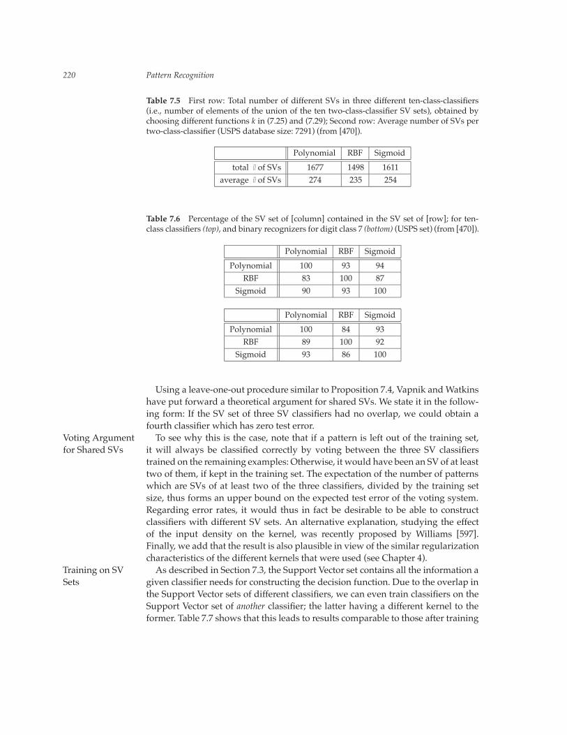
Table 7.5 First row: Total number of different SVs in three different ten-class-classifiers(i.e., number of elements of the union of the ten two-class-classifier SV sets), obtained bychoosing different functions k in (7.25) and (7.29); Second row: Average number of SVs pertwo-class-classifier (USPS database size: 7291) (from [470]).
Polynomial RBF Sigmoid
total # of SVs 1677 1498 1611average # of SVs 274 235 254
Table 7.6 Percentage of the SV set of [column] contained in the SV set of [row]; for ten-class classifiers (top), and binary recognizers for digit class 7 (bottom) (USPS set) (from [470]).
Polynomial RBF Sigmoid
Polynomial 100 93 94RBF 83 100 87
Sigmoid 90 93 100
Polynomial RBF Sigmoid
Polynomial 100 84 93RBF 89 100 92
Sigmoid 93 86 100
Using a leave-one-out procedure similar to Proposition 7.4, Vapnik andWatkinshave put forward a theoretical argument for shared SVs. We state it in the follow-ing form: If the SV set of three SV classifiers had no overlap, we could obtain afourth classifier which has zero test error.To see why this is the case, note that if a pattern is left out of the training set,Voting Argument
for Shared SVs it will always be classified correctly by voting between the three SV classifierstrained on the remaining examples: Otherwise, it would have been an SV of at leasttwo of them, if kept in the training set. The expectation of the number of patternswhich are SVs of at least two of the three classifiers, divided by the training setsize, thus forms an upper bound on the expected test error of the voting system.Regarding error rates, it would thus in fact be desirable to be able to constructclassifiers with different SV sets. An alternative explanation, studying the effectof the input density on the kernel, was recently proposed by Williams [597].Finally, we add that the result is also plausible in view of the similar regularizationcharacteristics of the different kernels that were used (see Chapter 4).As described in Section 7.3, the Support Vector set contains all the information aTraining on SV
Sets given classifier needs for constructing the decision function. Due to the overlap inthe Support Vector sets of different classifiers, we can even train classifiers on theSupport Vector set of another classifier; the latter having a different kernel to theformer. Table 7.7 shows that this leads to results comparable to those after training
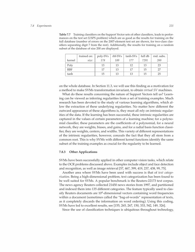
7.8 Experiments 221
Table 7.7 Training classifiers on the Support Vector sets of other classifiers, leads to perfor-mances on the test set (USPS problem) which are as good as the results for training on thefull database (number of errors on the 2007-element test set are shown, for two-class clas-sifiers separating digit 7 from the rest). Additionally, the results for training on a randomsubset of the database of size 200 are displayed.
trained on: poly-SVs rbf-SVs tanh-SVs full db rnd. subs.kernel size: 178 189 177 7291 200
Poly 13 13 12 13 23RBF 17 13 17 15 27tanh 15 13 13 15 25
on the whole database. In Section 11.3, we will use this finding as a motivation fora method to make SVMs transformation invariant, to obtain virtual SV machines.What do these results concerning the nature of Support Vectors tell us? Learn-
ing can be viewed as inferring regularities from a set of training examples. Muchresearch has been devoted to the study of various learning algorithms, which al-low the extraction of these underlying regularities. No matter how different theoutward appearance of these algorithms is, they must all rely on intrinsic regular-ities of the data. If the learning has been successful, these intrinsic regularities arecaptured in the values of certain parameters of a learning machine; for a polyno-mial classifier, these parameters are the coefficients of a polynomial, for a neuralnetwork, they are weights, biases, and gains, and for a radial basis function classi-fier, they are weights, centers, and widths. This variety of different representationsof the intrinsic regularities, however, conceals the fact that they all stem from acommon root. This is why SVMs with different kernel functions identify the samesubset of the training examples as crucial for the regularity to be learned.
7.8.3 Other Applications
SVMs have been successfully applied in other computer vision tasks, which relateto the OCR problems discussed above. Examples include object and face detectionand recognition, as well as image retrieval [57, 467, 399, 419, 237, 438, 99, 75].Another area where SVMs have been used with success is that of text catego-
rization. Being a high-dimensional problem, text categorization has been found tobe well suited for SVMs. A popular benchmark is the Reuters-22173 text corpus.The news agency Reuters collected 21450 news stories from 1997, and partitionedand indexed them into 135 different categories. The feature typically used to clas-sify Reuters documents are 104-dimensional vectors containing word frequencieswithin a document (sometimes called the “bag-of-words” representation of texts,as it completely discards the information on word ordering). Using this coding,SVMs have led to excellent results, see [155, 265, 267, 150, 333, 542, 149, 326].Since the use of classification techniques is ubiquitous throughout technology,
222 Pattern Recognition
we cannot give an exhaustive listing of all successful SVM applications. We thusconclude the list with some of the more exotic applications, such as in High-Energy-Physics [19, 558], in the monitoring of household appliances [390], inprotein secondary structure prediction [249], and, with rather intriguing results,in the design of decision feedback equalizers (DFE) in telephony [105].
7.9 Summary
This chapter introduced SV pattern recognition algorithms. The crucial idea isto use kernels to reduce a complex classification task to one that can be solvedwith separating hyperplanes. We discussed what kind of hyperplane should beconstructed in order to get good generalization performance, leading to the ideaof large margins. It turns out that the concept of large margins can be justifiedin a number of different ways, including arguments based on statistical learningtheory, and compression schemes. We described in detail how the optimal marginhyperplane can be obtained as the solution of a quadratic programming problem.We started with the linear case, where the hyperplane is constructed in the spaceof the inputs, and then moved on to the case where we use a kernel function tocompute dot products, in order to compute the hyperplane in a feature space.Two further extensions greatly increase the applicability of the approach. First,
to deal with noisy data, we introduced so-called slack variables in the optimizationproblem. Second, for problems that have more than just two classes, we describeda number of generalizations of the binary SV classifiers described initially.Finally, we reported applications and benchmark comparisons for the widely
used USPS handwritten digit task. SVMs turn out to work very well in this field,as well as in a variety of other domains mentioned briefly.
7.10 Problems
7.1 (Weight Vector Scaling �) Show that instead of the “1” on the right hand side of theseparation constraint (7.11), we can use any positive number � � 0, without changing theoptimal margin hyperplane solution. What changes in the soft margin case?
7.2 (Dual Perceptron Algorithm [175] ��) Kernelize the perceptron algorithm describedin footnote 1. Which of the patterns will appear in the expansion of the solution?
7.3 (Margin of Optimal Margin Hyperplanes [62] ��) Prove that the geometric mar-gin � of the optimal margin hyperplane can be computed from the solution � via
��2 �m
∑i�1
�i� (7.68)
7.10 Problems 223
Also prove that
��2 � 2W(�) � �w�2� (7.69)
Note that for these relations to hold true, � needs to be the solution of (7.29).
7.4 (Relationship Between �w� and the Geometrical Margin �) (i) Consider a sep-arating hyperplane in canonical form. Prove that the margin, measured perpendicularly tothe hyperplane, equals 1��w�, by considering two opposite points which precisely satisfy� �w� xi�� b�� 1.(ii) How does the corresponding statement look for the case of �-SVC? Use the con-
straint (7.41), and assume that all slack variables are 0.
7.5 (Compression Bound for Large Margin Classification ÆÆÆ) Formalize the ideasstated in Section 7.2: Assuming that the data are separable and lie in a ball of radius R,how many bits are necessary to encode the labels of the data by encoding the parametersof a hyperplane? Formulate a generalization error bound in terms of the compression ratioby using the analysis of Vapnik [561, Section 4.6]. Compare the resulting bound withTheorem 7.3. Take into account the eigenvalues of the Gram matrix, using the ideas offrom [604] (cf. Section 12.4).
7.6 (Positive Definiteness of the SVC Hessian �) From Definition 2.4, prove that thematrix Qi j :� (yiyjk(xi� xj))i j is positive definite.
7.7 (Geometric Interpretation of Duality in SVC [38] ��) Prove that the program-ming problem (7.10), (7.11) has the same solution as (7.22), provided the threshold b isadjusted such that the hyperplane bisects the shortest connection of the two convex hulls.Hint: Show that the latter is the dual of the former. Interpret the result geometrically.
7.8 (Number of Points Required to Define a Hyperplane �) From (7.22), argue thatno matter what the dimensionality of the space, there can always be situations where twotraining points suffice to determine the optimal hyperplane.
7.9 (In-Bound SVs in Soft Margin SVMs �) Prove that in-bound SVs lie exactly onthe margin. Hint: Use the KKT conditions, and proceed analogously to Section 7.3, whereit was shown that in the hard margin case, all SVs lie exactly on the margin.Argue, moreover, that bound SVs can lie both on or in the margin, and that they will
“usually” lie in the margin.
7.10 (Pattern-Dependent Regularization �) Derive a version of the soft margin classi-fication algorithm which uses different regularization constants Ci for each training exam-ple. Start from (7.35), replace the second term by 1
m ∑mi�1 Cii, and derive the dual. Discussboth the mathematical form of the result, and possible applications (cf. [462]).
7.11 (Uncertain Labels ��) In this chapter, we have been concerned mainly with the casewhere the patterns are assigned to one of two classes, i.e., y � ��1. Consider now the
224 Pattern Recognition
case where the assignment is not strict, i.e., y � [1� 1]. Modify the soft margin variantsof the SV algorithm, (7.34), (7.35) and (7.41), (7.40), such that
whenever y � 0, the corresponding pattern has effectively no influence
if all labels are in ��1, the original algorithm is recovered
if �y� 1, then the corresponding pattern has less influence than it would have for�y� � 1.
7.12 (SVMs vs. Parzen Windows ÆÆÆ) Develop algorithms that approximate the SVM(soft or hard margin) solution by starting from the ParzenWindows algorithm (Figure 1.1)and sparsifying the expansion of the solution.
7.13 (Squared Error SVC [111] ��) Derive a version of the soft margin classificationalgorithm which penalizes the errors quadratically. Start from (7.35), replace the secondterm by 1
m ∑mi�1 2i , and derive the dual. Compare the result to the usual C-SVM, both in
terms of algorithmic differences and in terms of robustness properties. Which algorithmwould you expect to work better for Gaussian-like noise, which one for noise with longertails (and thus more outliers) (cf. Chapter 3)?
7.14 (C-SVC with Group Error Penalty ��) Suppose the training data are partitionedinto � groups,
(x11� y11)� � � � � (x
m11 � ym11 )
......
(x1� � y1�)� � � � � (x
m�
�� ym�
�)� (7.70)
where x ji �� and yji � ��1 (it is understood that the index i runs over �1� 2� � � � � � and
the index j runs over �1� 2� � � � �mi).Suppose, moreover, that we would like to count a point as misclassified already if one
point belonging to the same group is misclassified.Design an SV algorithm where each group’s penalty equals the slack of the worst point
in that group.Hint: Use the objective function
12�w�2 �∑
iCii� (7.71)
and the constraints
yji � (�w� x ji
�� b) � 1 i� (7.72)
i � 0� (7.73)
Show that the dual problem consists of maximizing
W(�) �∑i� j� ji
12 ∑i� j�i� � j�
� ji�j�
i� yji yj�
i�
�x ji � x
j�
i�
�� (7.74)
7.10 Problems 225
subject to
0 �∑i� j�ji yji � 0 �
ji � and ∑
j�ji Ci� (7.75)
Argue that typically, only one point per group will become an SV.Show that C-SVC is a special case of this algorithm.
7.15 (�-SVC with Group Error Penalty ���) Derive a �-version of the algorithm inProblem 7.14.
7.16 (C-SVC vs. �-SVC ��) As a modification of �-SVC (Section 7.5), compute the dualof � (w� �� �) � �w�2�2� C(��� (1�m)∑mi�1 i) (note that in �-SVC, C � 1 is used).Argue that due to the homogeneity of the objective function, the dual solution gets scaledby C, however, the decision function will not change. Hence we may set C � 1.
7.17 (Multi-class vs. Binary SVC [593] ��) (i) Prove that the multi-class SVC formu-lation of (7.59) specializes to the binary C-SVC (7.35) in the case k � 2, by usingw1 �w2, b1 �b2, and i � 1
2ri for pattern xi in class r. (ii) Derive the dual of (7.59).
7.18 (Multi-Class �-SVC ÆÆÆ) Derive a �-version of the approach described in Sec-tion 7.6.4.
7.19 (LPM with Constrained Signs �) Modify the LPM algorithm such that it is guar-anteed that each expansion pattern will have a coefficient i whose sign equals the classlabel yi. Hint: Do not introduce additional constraints, but eliminate the ��
i variables anduse a different ansatz for the solution.
7.20 (Multi-Class LPM [593] ��) In analogy to Section 7.6.4, develop a multi-class ver-sion of the LP machine (Section 7.7).
7.21 (Version Space [368, 239, 451, 238] ���) Consider hyperplanes passing throughthe origin, �x� �w� x� � 0, with weight vectors w ����w� � 1. The set of all such hy-perplanes forms a unit sphere in weight space. Each training example (x� y) �����1splits the sphere into two halves: one that correctly classifies (x� y), i.e., sgn �w� x� � y,and one that does not. Each training example thus corresponds to a hemisphere (or, equiv-alently, an oriented great circle) in weight space, and a training set (x1� y1)� � � � � (xm� ym)corresponds to the intersection of m hemispheres, called the version space.
1. Discuss how the distances between the training example and the hyperplane in the tworepresentations are related.
2. Discuss the relationship to the idea of the Hough transform [255]. The Hough transformis sometimes used in image processing to detect lines. In a nutshell, each point gets to castvotes in support for all potential lines that are consistent with it, and at the end, the linescan be read off the histogram of votes.
3. Prove that if all xi have the same norm, the maximummargin weight vector correspondsto the center of the largest m 1-dimensional sphere that fits into version space.
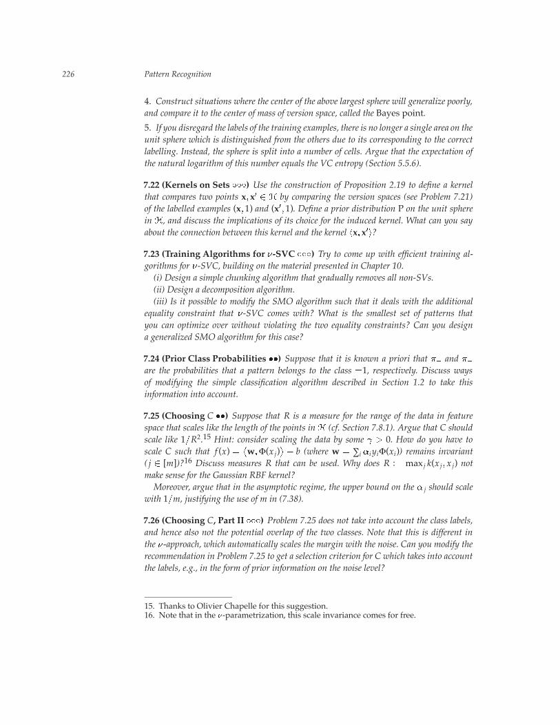
226 Pattern Recognition
4. Construct situations where the center of the above largest sphere will generalize poorly,and compare it to the center of mass of version space, called the Bayes point.
5. If you disregard the labels of the training examples, there is no longer a single area on theunit sphere which is distinguished from the others due to its corresponding to the correctlabelling. Instead, the sphere is split into a number of cells. Argue that the expectation ofthe natural logarithm of this number equals the VC entropy (Section 5.5.6).
7.22 (Kernels on Sets ÆÆÆ) Use the construction of Proposition 2.19 to define a kernelthat compares two points x� x� � � by comparing the version spaces (see Problem 7.21)of the labelled examples (x� 1) and (x�� 1). Define a prior distribution P on the unit spherein �, and discuss the implications of its choice for the induced kernel. What can you sayabout the connection between this kernel and the kernel �x� x��?
7.23 (Training Algorithms for �-SVC ÆÆÆ) Try to come up with efficient training al-gorithms for �-SVC, building on the material presented in Chapter 10.(i) Design a simple chunking algorithm that gradually removes all non-SVs.(ii) Design a decomposition algorithm.(iii) Is it possible to modify the SMO algorithm such that it deals with the additional
equality constraint that �-SVC comes with? What is the smallest set of patterns thatyou can optimize over without violating the two equality constraints? Can you designa generalized SMO algorithm for this case?
7.24 (Prior Class Probabilities ��) Suppose that it is known a priori that �� and ��
are the probabilities that a pattern belongs to the class �1, respectively. Discuss waysof modifying the simple classification algorithm described in Section 1.2 to take thisinformation into account.
7.25 (Choosing C ��) Suppose that R is a measure for the range of the data in featurespace that scales like the length of the points in� (cf. Section 7.8.1). Argue that C shouldscale like 1�R2.15 Hint: consider scaling the data by some � � 0. How do you have toscale C such that f (x) �
�w�Φ(xj)
�� b (where w � ∑i �i yiΦ(xi)) remains invariant
( j � [m])?16 Discuss measures R that can be used. Why does R :� max j k(xj� xj) notmake sense for the Gaussian RBF kernel?Moreover, argue that in the asymptotic regime, the upper bound on the � j should scale
with 1�m, justifying the use of m in (7.38).
7.26 (Choosing C, Part II ÆÆÆ) Problem 7.25 does not take into account the class labels,and hence also not the potential overlap of the two classes. Note that this is different inthe �-approach, which automatically scales the margin with the noise. Can you modify therecommendation in Problem 7.25 to get a selection criterion for C which takes into accountthe labels, e.g., in the form of prior information on the noise level?
15. Thanks to Olivier Chapelle for this suggestion.16. Note that in the �-parametrization, this scale invariance comes for free.