Chapter 7

Homogeneous Equations andLinearly Independent Vectors

In the preceding chapter we have developed methods for solving sets of n linearequations in n unknowns which are of the form Axxx = bbb. Cramer’s rule was foundto provide a formula for the unique solution of such equations if det(A) �= 0, butGaussian elimination is also able to provide solutions in this case, as well as thosewhere det(A) = 0, where there are either no solutions or infinitely many solutions.

In this chapter, we examine solutions of the associated homogeneous equationAxxx = 000 corresponding to the original inhomogeneous equation Axxx = bbb. Solutionsto the homogeneous equation will be seen to occur naturally when det(A) = 0. Webegin this chapter with examples that illustrate this, which will also provide ad-ditional practice in using the method of Gaussian elimination. This will motivatea general expression of solutions of an inhomogeneous equations as the sum of aparticular solution of the inhomogeneous equation (a point in Rn) and a solutionof the homogeneous equation (a line, plane, or hyperplane in Rn that contains theparticular solution). This leads to the concept of linearly dependent and linearlyindependent vectors – one of the most important in vector analysis. This will es-tablish a conceptual foundation for understanding the conditions that determinethe nature of the solutions of the general linear equation Axxx = bbb from a more in-tuitive perspective, as well as providing additional insight into the meaning of thedeterminant.

An adjunct to linear independence is the notion of a ‘natural basis,’ whichprovides the simplest and most convenient set of n vectors in terms of which allother vectors in Rn can be expressed. These vectors have unit length, are mutuallyperpendicular and are the generalization to higher dimensions of the unit vectorsiii, jjj, and kkk in R3.

91

92 Linear Algebra

7.1 IntroductionTo motivate the representation of solutions of systems of equations Axxx = bbb whendet(A) = 0 in the form described in the introduction, we consider two examples.

EXAMPLE 7.1. Consider the following system of 3 equations in 3 unknowns:

x−2y−3z = 2,x−4y−13z = 14,

−3x+5y+4z = 0.(7.1)

The determinant of the matrix of coefficients is calculated as��������

1 −2 −3

1 −4 −13

−3 5 4

��������=−16−78−15− (−36)− (−8)− (65) = 0, (7.2)

so there is no unique solution to the system of equations (7.1). The solution canbe obtained by Gaussian elimination. Beginning with

1 −2 −3 21 −4 −13 14

−3 5 4 0

, (7.3)

we subtract the first row from the second row and add 3 times the first row to thethird row:

1 −2 −3 20 −2 −10 120 −1 −5 6

. (7.4)

We then subtract twice the third row from each of the first and second rows:

1 0 7 −100 0 0 00 −1 −5 6

. (7.5)

Finally, we multiply the third row by −1 and exchange the second and third rowsto obtain

1 0 7 −100 1 5 −60 0 0 0

. (7.6)

Homogeneous Equations and Independent Vectors 93

The transcription of this matrix into equation form is

x+7z = −10,y+5z = −6.

(7.7)

We have two equations in three unknowns, so we do not have a unique solution aswe have one degree of freedom. If we set z = λ , where λ ∈ R, we can write thesolution as

x

y

z

=

−10−7λ−6−5λ

λ

=

−10

−6

0

+λ

−7

−5

1

. (7.8)

By defining

xxx0 ≡

−10

−6

0

, xxx1 ≡

−7

−5

1

, (7.9)

we can write (7.8) asxxx = xxx0 +λxxx1 , (7.10)

which is the equation of a line (cf. (4.1)). Thus, we have an infinity of solutionsthat are parametrized by λ .

We now consider the quantities Axxx0 and Axxx1:

Axxx0 =

1 −2 −3

1 −4 −13

−3 5 4

−10

−6

0

=

2

14

0

= bbb , (7.11)

Axxx1 =

1 −2 −3

1 −4 −13

−3 5 4

−7

−5

1

=

0

0

0

= 000. (7.12)

The vector xxx1 is a solution of the homogeneous equation, and xxx0 is a particularsolution of (7.1). Hence, we have

Axxx = A(xxx0 +λxxx1) = Axxx0 +λAxxx1 = bbb . (7.13)

94 Linear Algebra

EXAMPLE 7.2. Consider the following system of 3 equations in 3 unknowns:

2x+4y−6z = 6,3x+6y−9z = 9,−x−2y+3z = −3.

(7.14)

The determinant of the matrix of coefficients,��������

2 4 −6

3 6 −9

−1 −2 3

��������= 36+36+36−36−36−36 = 0, (7.15)

so there is no unique solution to the system of equations (7.14). Gaussian elimi-nation proceeds by first writing

2 4 −6 63 6 −9 9

−1 −2 3 −3

. (7.16)

Adding 2 times row 3 to row 1 and 3 times row 3 to row 2,

0 0 0 00 0 0 0

−1 −2 3 −3

, (7.17)

multiplying the third row by −1 and exchanging the first and third rows yields,

1 2 −3 30 0 0 00 0 0 0

. (7.18)

When transcribed into an equation, Gaussian elimination yields a single constraintamong three unknowns:

x+2y−3z = 3, (7.19)which is the equation of a plane (cf. (4.20)). There are two degrees of freedom,which we take as y = λ and z = µ for λ , µ ∈ R. The solutions to (7.14) can bewritten as

x

y

z

=

−2λ +3µ +3

λµ

=

3

0

0

+λ

−2

1

0

+µ

3

0

1

. (7.20)

Homogeneous Equations and Independent Vectors 95

By defining

xxx0 ≡

3

0

0

, xxx1 ≡

−2

1

0

, xxx2 ≡

3

0

1

, (7.21)

we can write (7.20) succinctly as

xxx = xxx0 +λx1 +µxxx2 . (7.22)

Finally, the quantities Axxx0, Axxx1, Axxx2 are calculated as

Axxx0 =

2 4 −6

3 6 −9

−1 −2 3

3

0

0

=

6

9

−1

= bbb , (7.23)

Axxx1 =

2 4 −6

3 6 −9

−1 −2 3

−2

1

0

=

0

0

0

= 000, (7.24)

Axxx2 =

2 4 −6

3 6 −9

−1 −2 3

3

0

1

=

0

0

0

= 000. (7.25)

We again see that xxx1 and xxx2 are solutions of the homogeneous equation Axxx = 000,and xxx0 is a particular solution of the original system Axxx = bbb in (7.14).

7.2 The Homogeneous EquationThe examples in the preceding section suggest that, for 3×3 systems of equationsAxxx = bbb whose determinant of the matrix of coefficients vanishes, the infinity ofsolutions can be written as the sum of a particular solution to this equation andsolution(s) of the associated homogeneous equation Axxx = 000. In this section, weshow that this result can be generalized to n× n systems of equations with in-finitely many solutions. We first formalize our discussion with a definition.

DEFINITION 7.1. The n-dimensional zero vector xxx = 000 is always a solution ofany system of n homogeneous equation in n unknowns: A000 = 000. This is called thetrivial solution. Any other solution of these equations is called non-trivial.

96 Linear Algebra

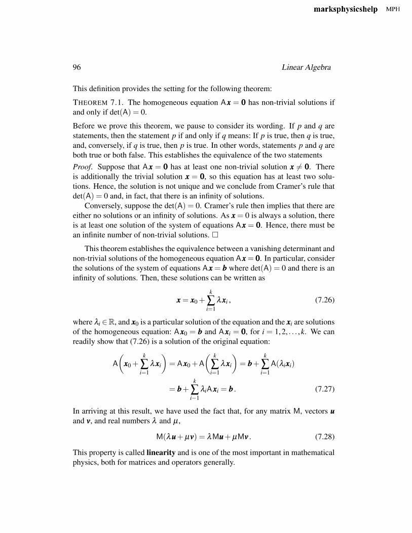
This definition provides the setting for the following theorem:

THEOREM 7.1. The homogeneous equation Axxx = 000 has non-trivial solutions ifand only if det(A) = 0.

Before we prove this theorem, we pause to consider its wording. If p and q arestatements, then the statement p if and only if q means: If p is true, then q is true,and, conversely, if q is true, then p is true. In other words, statements p and q areboth true or both false. This establishes the equivalence of the two statementsProof. Suppose that Axxx = 000 has at least one non-trivial solution xxx �= 000. Thereis additionally the trivial solution xxx = 000, so this equation has at least two solu-tions. Hence, the solution is not unique and we conclude from Cramer’s rule thatdet(A) = 0 and, in fact, that there is an infinity of solutions.

Conversely, suppose the det(A) = 0. Cramer’s rule then implies that there areeither no solutions or an infinity of solutions. As xxx = 0 is always a solution, thereis at least one solution of the system of equations Axxx = 000. Hence, there must bean infinite number of non-trivial solutions. �

This theorem establishes the equivalence between a vanishing determinant andnon-trivial solutions of the homogeneous equation Axxx = 000. In particular, considerthe solutions of the system of equations Axxx = bbb where det(A) = 0 and there is aninfinity of solutions. Then, these solutions can be written as

xxx = xxx0 +k

∑i=1

λxxxi , (7.26)

where λi ∈R, and xxx0 is a particular solution of the equation and the xxxi are solutionsof the homogeneous equation: Axxx0 = bbb and Axxxi = 000, for i = 1,2, . . . ,k. We canreadily show that (7.26) is a solution of the original equation:

A

�xxx0 +

k

∑i=1

λxxxi

�= Axxx0 +A

� k

∑i=1

λxxxi

�= bbb+

k

∑i=1

A(λixxxi)

= bbb+k

∑i−1

λiAxxxi = bbb . (7.27)

In arriving at this result, we have used the fact that, for any matrix M, vectors uuuand vvv, and real numbers λ and µ ,

M(λuuu+µvvv) = λMuuu+µMvvv . (7.28)

This property is called linearity and is one of the most important in mathematicalphysics, both for matrices and operators generally.

Homogeneous Equations and Independent Vectors 97

7.3 Linearly Dependent and Independent VectorsOur discussion of systems of linearly equations has focussed on determining thecondition for different types of solutions and finding those solutions either byCramer’s method or, more generally, with Gaussian elimination. In this section,we adopt amore geometric approach to explain how these results can be under-stood in terms of vectors.

Consider a matrix

A=

a11 a12 · · · a1 j · · · a1n

a21 a22 · · · a2 j · · · a2n...

... . . . ... . . . ...ai1 ai2 · · · ai j · · · ain...

... . . . ... . . . ...an1 an2 · · · a2 j · · · ann

. (7.29)

We can view the entries in each column as the components of a column vector,just as we did when proving Cramer’s rule in Sec. 6.2. Accordingly, we define

AAA1 ≡

a11

a12...

ai1...

an1

, AAA2 ≡

a12

a22...

ai2...

an2

, AAA j ≡

a1 j

a2 j...

ai j...

an j

, AAAn ≡

a1n

a2n...

ain...

ann

,

(7.30)which enables us to write A as

A= (AAA1,AAA2, . . . ,AAA j, . . . ,AAAn) . (7.31)

In particular, a system of n simultaneous homogeneous equations in n unknowns,

a11x1 + a12x2 + · · · + a1 j + · · · + a1n = 0,a21x1 + a22x2 + · · · + a2 jx j + · · · + a2nxn = 0,

...... . . . ... . . . ...

...ai1x1 + ai2x2 + · · · + ai jx j + · · · + ainxn = 0,

...... . . . ... . . . ...

...an1x1 + an2x2 + · · · + an jx j + · · · + annxn = 0,

(7.32)

98 Linear Algebra

can be written concisely as

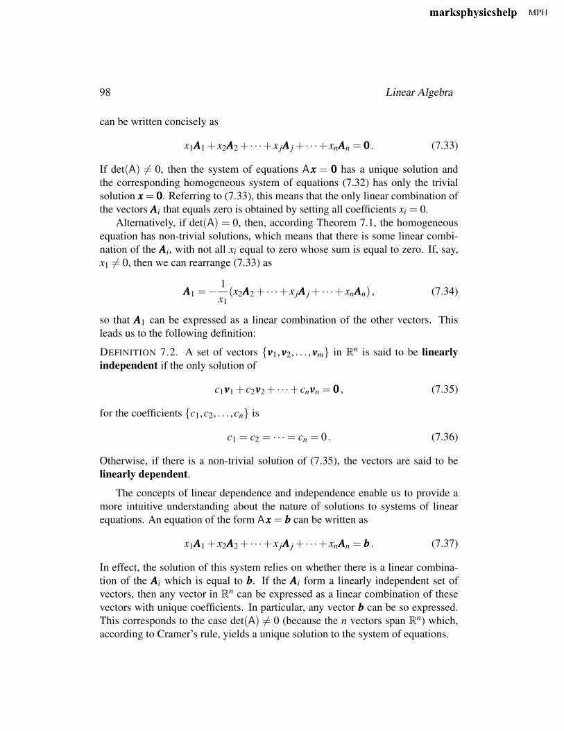
x1AAA1 + x2AAA2 + · · ·+ x jAAA j + · · ·+ xnAAAn = 000. (7.33)

If det(A) �= 0, then the system of equations Axxx = 000 has a unique solution andthe corresponding homogeneous system of equations (7.32) has only the trivialsolution xxx = 000. Referring to (7.33), this means that the only linear combination ofthe vectors AAAi that equals zero is obtained by setting all coefficients xi = 0.

Alternatively, if det(A) = 0, then, according Theorem 7.1, the homogeneousequation has non-trivial solutions, which means that there is some linear combi-nation of the AAAi, with not all xi equal to zero whose sum is equal to zero. If, say,x1 �= 0, then we can rearrange (7.33) as

AAA1 =− 1x1(x2AAA2 + · · ·+ x jAAA j + · · ·+ xnAAAn) , (7.34)

so that AAA1 can be expressed as a linear combination of the other vectors. Thisleads us to the following definition:

DEFINITION 7.2. A set of vectors {vvv1,vvv2, . . . ,vvvm} in Rn is said to be linearlyindependent if the only solution of

c1vvv1 + c2vvv2 + · · ·+ cnvvvn = 000, (7.35)

for the coefficients {c1,c2, . . . ,cn} is

c1 = c2 = · · ·= cn = 0. (7.36)

Otherwise, if there is a non-trivial solution of (7.35), the vectors are said to belinearly dependent.

The concepts of linear dependence and independence enable us to provide amore intuitive understanding about the nature of solutions to systems of linearequations. An equation of the form Axxx = bbb can be written as

x1AAA1 + x2AAA2 + · · ·+ x jAAA j + · · ·+ xnAAAn = bbb . (7.37)

In effect, the solution of this system relies on whether there is a linear combina-tion of the AAAi which is equal to bbb. If the AAAi form a linearly independent set ofvectors, then any vector in Rn can be expressed as a linear combination of thesevectors with unique coefficients. In particular, any vector bbb can be so expressed.This corresponds to the case det(A) �= 0 (because the n vectors span Rn) which,according to Cramer’s rule, yields a unique solution to the system of equations.

Homogeneous Equations and Independent Vectors 99

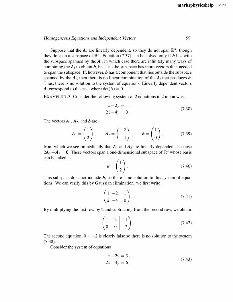
Suppose that the AAAi are linearly dependent, so they do not span Rn, thoughthey do span a subspace of Rn. Equation (7.37) can be solved only if bbb lies withthe subspace spanned by the AAAi, in which case there are infinitely many ways ofcombining the AAAi to obtain bbb, because the subspace has more vectors than neededto span the subspace. If, however, bbb has a component that lies outside the subspacespanned by the AAAi, then there is no linear combination of the AAAi that produces bbb.Thus, there is no solution to the system of equations. Linearly dependent vectorsAAAi correspond to the case where det(A) = 0.

EXAMPLE 7.3. Consider the following system of 2 equations in 2 unknowns:

x−2y = 1,2x−4y = 0.

(7.38)

The vectors AAA1, AAA2, and bbb are

AAA1 =

�1

2

�, AAA2 =

�−2

−4

�, bbb =

�1

0

�, (7.39)

from which we see immediately that AAA1 and AAA2 are linearly dependent, because2AAA1 +AAA2 = 000. These vectors span a one-dimensional subspace of R2 whose basiscan be taken as

uuu =

�1

2

�. (7.40)

This subspace does not include bbb, so there is no solution to this system of equa-tions. We can verify this by Gaussian elimination. we first write

�1 −2 12 −4 0

�. (7.41)

By multiplying the first row by 2 and subtracting from the second row, we obtain�

1 −2 10 0 −2

�. (7.42)

The second equation, 0 =−2 is clearly false so there is no solution to the system(7.38).

Consider the system of equations

x−2y = 3,2x−4y = 6,

(7.43)

100 Linear Algebra

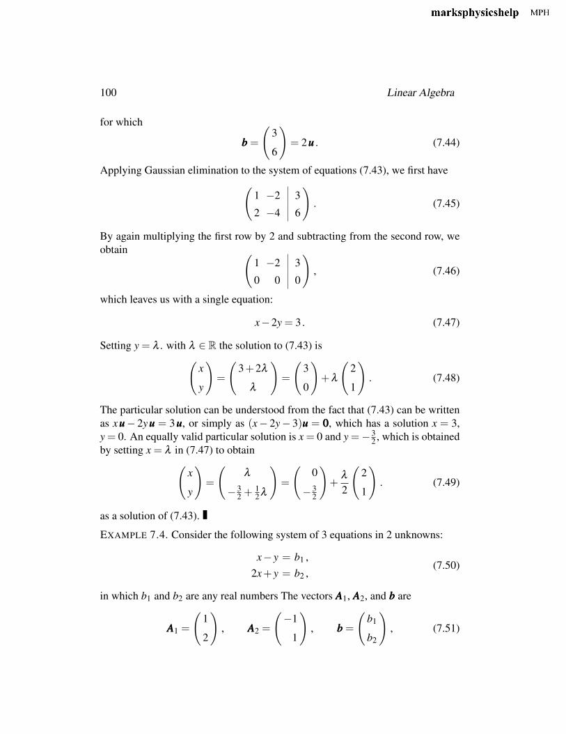
for which

bbb =

�3

6

�= 2uuu . (7.44)

Applying Gaussian elimination to the system of equations (7.43), we first have�

1 −2 32 −4 6

�. (7.45)

By again multiplying the first row by 2 and subtracting from the second row, weobtain �

1 −2 30 0 0

�, (7.46)

which leaves us with a single equation:

x−2y = 3. (7.47)

Setting y = λ . with λ ∈ R the solution to (7.43) is�

x

y

�=

�3+2λ

λ

�=

�3

0

�+λ

�2

1

�. (7.48)

The particular solution can be understood from the fact that (7.43) can be writtenas xuuu− 2yuuu = 3uuu, or simply as (x− 2y− 3)uuu = 000, which has a solution x = 3,y = 0. An equally valid particular solution is x = 0 and y =−3

2 , which is obtainedby setting x = λ in (7.47) to obtain

�x

y

�=

�λ

−32 +

12λ

�=

�0

−32

�+

λ2

�2

1

�. (7.49)

as a solution of (7.43).

EXAMPLE 7.4. Consider the following system of 3 equations in 2 unknowns:

x− y = b1 ,2x+ y = b2 ,

(7.50)

in which b1 and b2 are any real numbers The vectors AAA1, AAA2, and bbb are

AAA1 =

�1

2

�, AAA2 =

�−1

1

�, bbb =

�b1

b2

�, (7.51)

Homogeneous Equations and Independent Vectors 101

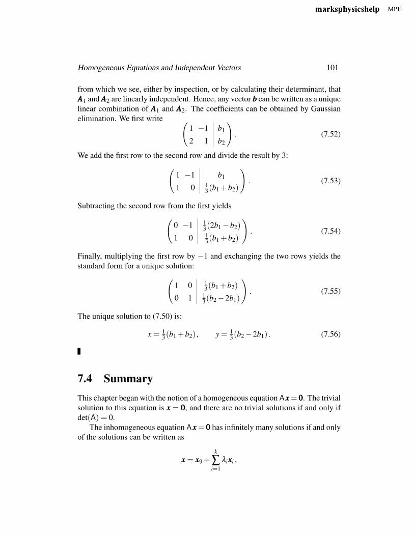
from which we see, either by inspection, or by calculating their determinant, thatAAA1 and AAA2 are linearly independent. Hence, any vector bbb can be written as a uniquelinear combination of AAA1 and AAA2. The coefficients can be obtained by Gaussianelimination. We first write �

1 −1 b1

2 1 b2

�. (7.52)

We add the first row to the second row and divide the result by 3:�

1 −1 b1

1 0 13(b1 +b2)

�. (7.53)

Subtracting the second row from the first yields�

0 −1 13(2b1 −b2)

1 0 13(b1 +b2)

�. (7.54)

Finally, multiplying the first row by −1 and exchanging the two rows yields thestandard form for a unique solution:

�1 0 1

3(b1 +b2)

0 1 13(b2 −2b1)

�. (7.55)

The unique solution to (7.50) is:

x = 13(b1 +b2) , y = 1

3(b2 −2b1) . (7.56)

7.4 SummaryThis chapter began with the notion of a homogeneous equation Axxx= 000. The trivialsolution to this equation is xxx = 000, and there are no trivial solutions if and only ifdet(A) = 0.

The inhomogeneous equation Axxx = 000 has infinitely many solutions if and onlyof the solutions can be written as

xxx = xxx9 +k

∑i=1

λixxxi ,

102 Linear Algebra

where Axxx0 = bbb, λi ∈ R, and Axxxi = 000, for i = 1,2, . . . ,k.A set of vectors {vvv1,vvv2, . . . ,vvvm} in R is linearly dependent of there exist num-

bers c1,c2, . . . ,cm, not all zero, such that

c1vvv1 + c2vvv2 + · · ·+ cmvvvm = 000.

A set of vectors {vvv1,vvv2, . . . ,vvvm} in R is linearly independent if

c1vvv1 + c2vvv2 + · · ·+ cmvvvm = 000

implies that c1 = c2 = · · ·= cm = 0.