chapter 7 estimation - mmathematics€¦ · the standard normal distribution"inchapter 5...

Chapter 7

Estimation

If we wish to estimate the mean μ of a population for which a census is impractical,say the average height of all 18-year-old men in the country, a reasonable strategyis to take a sample, compute its mean x⎯⎯, and estimate the unknown number μ bythe known number x⎯⎯. For example, if the average height of 100 randomly selectedmen aged 18 is 70.6 inches, then we would say that the average height of all18-year-old men is (at least approximately) 70.6 inches.

Estimating a population parameter by a single number like this is called pointestimation; in the case at hand the statistic x⎯⎯ is a point estimate of the parameterμ. The terminology arises because a single number corresponds to a single point onthe number line.

A problem with a point estimate is that it gives no indication of how reliable theestimate is. In contrast, in this chapter we learn about interval estimation. In brief,in the case of estimating a population mean μ we use a formula to compute fromthe data a number E, called the margin of error1 of the estimate, and form theinterval [x⎯⎯ − E, x⎯⎯ + E] .We do this in such a way that a certain proportion, say95%, of all the intervals constructed from sample data by means of this formulacontain the unknown parameter μ. Such an interval is called a 95% confidenceinterval2 for μ.

Continuing with the example of the average height of 18-year-old men, supposethat the sample of 100 men mentioned above for which x⎯⎯ = 70.6 inches also hadsample standard deviation s = 1.7 inches. It then turns out that E = 0.33 and wewould state that we are 95% confident that the average height of all 18-year-oldmen is in the interval formed by 70.6 ± 0.33 inches, that is, the average is between70.27 and 70.93 inches. If the sample statistics had come from a smaller sample, saya sample of 50 men, the lower reliability would show up in the 95% confidenceinterval being longer, hence less precise in its estimate. In this example the 95%confidence interval for the same sample statistics but with n = 50 is 70.6 ± 0.47inches, or from 70.13 to 71.07 inches.

1. E, the number added to andsubtracted from the pointestimate to produce theinterval estimate.

2. An interval with endpointsx⎯⎯ ± E, computed from thesample data in such a way thata specified proportion of allintervals constructed by thisprocess will contain theparameter of interest.

325

7.1 Large Sample Estimation of a Population Mean

LEARNING OBJECTIVES

1. To become familiar with the concept of an interval estimate of thepopulation mean.

2. To understand how to apply formulas for a confidence interval for apopulation mean.

The Central Limit Theorem says that, for large samples (samples of size n ≥ 30),when viewed as a random variable the sample mean X

⎯⎯ is normally distributed with

mean μX⎯ ⎯⎯ = μ and standard deviation σX⎯ ⎯⎯ = σ / n⎯⎯

√ .The Empirical Rule says that

we must go about two standard deviations from the mean to capture 95% of thevalues of X⎯⎯ generated by sample after sample. A more precise distance based on the

normality of X⎯⎯ is 1.960 standard deviations, which is E = 1.960σ / n⎯⎯

√ .

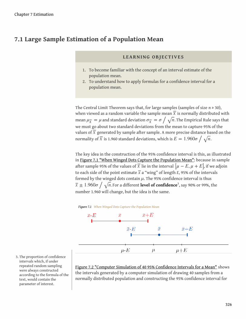
The key idea in the construction of the 95% confidence interval is this, as illustratedin Figure 7.1 "When Winged Dots Capture the Population Mean": because in sampleafter sample 95% of the values of X⎯⎯ lie in the interval [μ − E, μ + E], if we adjointo each side of the point estimate x⎯⎯ a “wing” of length E, 95% of the intervalsformed by the winged dots contain μ. The 95% confidence interval is thus

x⎯⎯ ± 1.960σ / n⎯⎯

√ .For a different level of confidence3, say 90% or 99%, the

number 1.960 will change, but the idea is the same.

Figure 7.1 When Winged Dots Capture the Population Mean

Figure 7.2 "Computer Simulation of 40 95% Confidence Intervals for a Mean" showsthe intervals generated by a computer simulation of drawing 40 samples from anormally distributed population and constructing the 95% confidence interval for

3. The proportion of confidenceintervals which, if underrepeated random samplingwere always constructedaccording to the formula of thetext, would contain theparameter of interest.

Chapter 7 Estimation

326

each one. We expect that about (0.05) (40) = 2of the intervals so constructed

would fail to contain the population mean μ, and in this simulation two of theintervals, shown in red, do.

Figure 7.2 Computer Simulation of 40 95% Confidence Intervals for a Mean

It is standard practice to identify the level of confidence in terms of the area α inthe two tails of the distribution of X⎯⎯ when the middle part specified by the level ofconfidence is taken out. This is shown in Figure 7.3, drawn for the general situation,and in Figure 7.4, drawn for 95% confidence. Remember from Section 5.4.1 "Tails ofthe Standard Normal Distribution" in Chapter 5 "Continuous Random Variables"that the z-value that cuts off a right tail of area c is denoted zc. Thus the number

1.960 in the example is z.025 , which is zα∕2 for α = 1 − 0.95 = 0.05.


7.1 Large Sample Estimation of a Population Mean 327

Figure 7.3

For 100 (1 − α)% confidence the area in each tail is α ∕ 2.

Figure 7.4

For 95% confidence the area in each tail is α ∕ 2 = 0.025.



The level of confidence can be any number between 0 and 100%, but the mostcommon values are probably 90% (α = 0.10), 95% (α = 0.05), and 99% (α = 0.01).

Thus in general for a 100 (1 − α)% confidence interval, E = zα∕2 (σ / n⎯⎯

√ ), so

the formula for the confidence interval is x⎯⎯ ± zα∕2 (σ / n⎯⎯

√ ) .While sometimes

the population standard deviation σ is known, typically it is not. If not, for n ≥ 30 itis generally safe to approximate σ by the sample standard deviation s.

Large Sample 100 (1 − α)% Confidence Interval for aPopulation Mean

If σ is known: x⎯⎯ ± zα∕2

σ

n√

If σ is unknown: x⎯⎯ ± zα∕2

s

n√

A sample is considered large when n ≥ 30.

As mentioned earlier, the number E = zα∕2σ / n⎯⎯

√ or E = zα∕2s / n⎯⎯

√ is called

the margin of error of the estimate.



EXAMPLE 1

Find the number zα∕2 needed in construction of a confidence interval:

a. when the level of confidence is 90%;b. when the level of confidence is 99%.

Solution:

a. For confidence level 90%, α = 1 − 0.90 = 0.10 , so zα∕2 = z0.05 .The procedure for finding this number was given in Section 5.4.1 "Tailsof the Standard Normal Distribution". Since the area under the standardnormal curve to the right of z.05 is 0.05, the area to the left of z0.05 is0.95. We search for the area 0.9500 in Figure 12.2 "Cumulative NormalProbability". The closest entries in the table are 0.9495 and 0.9505,corresponding to z-values 1.64 and 1.65. Since 0.95 is exactly halfwaybetween 0.9495 and 0.9505 we use the average 1.645 of the z-values forz0.05.

b. For confidence level 99%, α = 1 − 0.99 = 0.01 , so zα∕2 = z0.005 .Since the area under the standard normal curve to the right of z0.005 is0.005, the area to the left of z0.005 is 0.9950. We search for the area 0.9950in Figure 12.2 "Cumulative Normal Probability". The closest entries inthe table are 0.9949 and 0.9951, corresponding to z-values 2.57 and 2.58.Since 0.995 is halfway between 0.9949 and 0.9951 we use the average2.575 of the z-values for z0.005.



EXAMPLE 2

Use Figure 12.3 "Critical Values of " to find the number zα∕2 needed inconstruction of a confidence interval:

a. when the level of confidence is 90%;b. when the level of confidence is 99%.

Solution:

a. In the next section we will learn about a continuous random variablethat has a probability distribution called the Student t-distribution.Figure 12.3 "Critical Values of " gives the value tc that cuts off a right tailof area c for different values of c. The last line of that table, the one

whose heading is the symbol ∞ for infinity and [z], gives thecorresponding z-value zc that cuts off a right tail of the same area c. Inparticular, z0.05 is the number in that row and in the column with theheading t0.05. We read off directly that z0.05 = 1.645.

b. In Figure 12.3 "Critical Values of " z0.005 is the number in the last rowand in the column headed t0.005, namely 2.576.

Figure 12.3 "Critical Values of " can be used to find zc only for those values of c for

which there is a column with the heading tc appearing in the table; otherwise we

must use Figure 12.2 "Cumulative Normal Probability" in reverse. But when it canbe done it is both faster and more accurate to use the last line of Figure 12.3"Critical Values of " to find zc than it is to do so using Figure 12.2 "Cumulative

Normal Probability" in reverse.



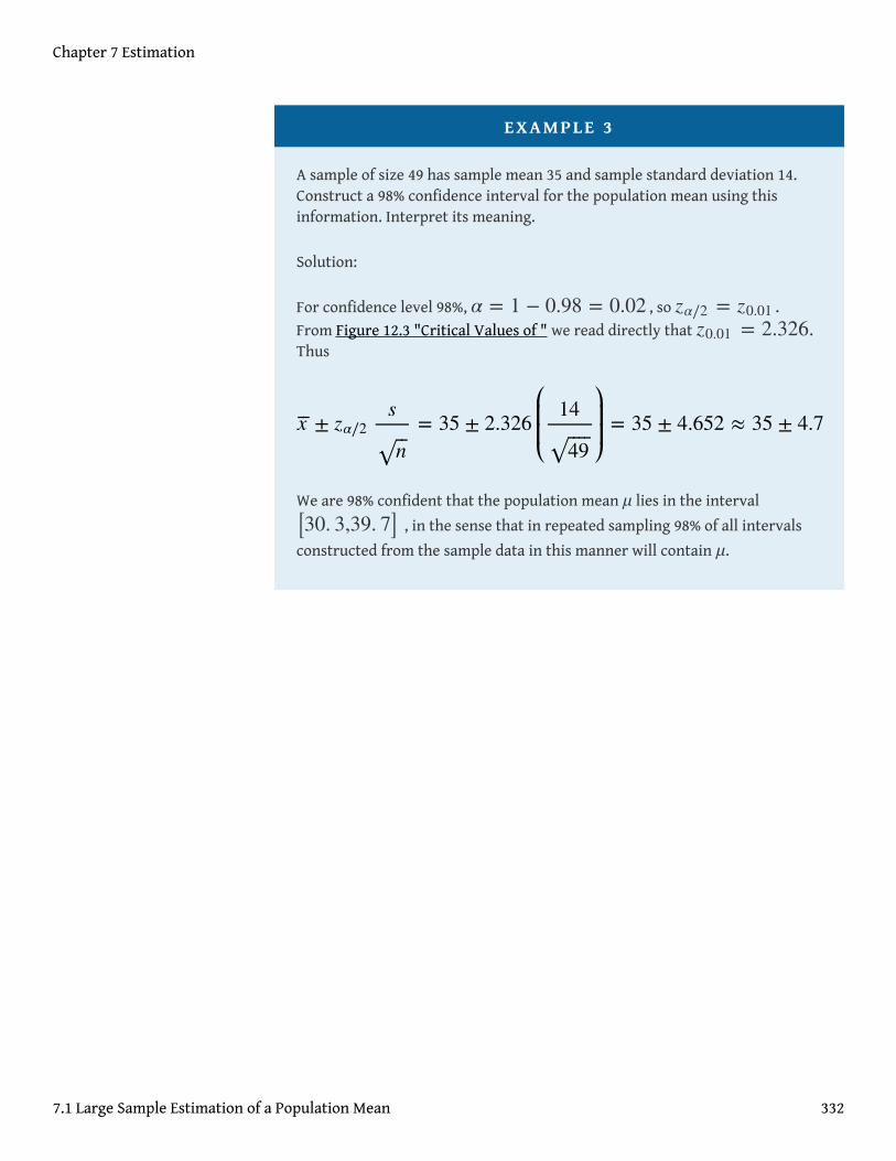
EXAMPLE 3

A sample of size 49 has sample mean 35 and sample standard deviation 14.Construct a 98% confidence interval for the population mean using thisinformation. Interpret its meaning.

Solution:

For confidence level 98%, α = 1 − 0.98 = 0.02 , so zα∕2 = z0.01 .From Figure 12.3 "Critical Values of " we read directly that z0.01 = 2.326.Thus

We are 98% confident that the population mean μ lies in the interval

[30. 3,39. 7] , in the sense that in repeated sampling 98% of all intervals

constructed from the sample data in this manner will contain μ.

x⎯⎯ ± zα∕2s

n⎯⎯

√= 35 ± 2.326

14

49⎯ ⎯⎯⎯

√

= 35 ± 4.652 ≈ 35 ± 4.7



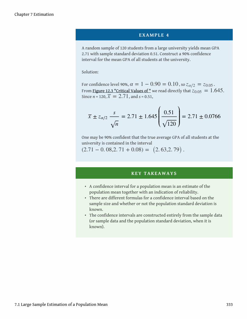
EXAMPLE 4

A random sample of 120 students from a large university yields mean GPA2.71 with sample standard deviation 0.51. Construct a 90% confidenceinterval for the mean GPA of all students at the university.

Solution:

For confidence level 90%, α = 1 − 0.90 = 0.10 , so zα∕2 = z0.05 .From Figure 12.3 "Critical Values of " we read directly that z0.05 = 1.645.Since n = 120, x⎯⎯ = 2.71, and s = 0.51,

One may be 90% confident that the true average GPA of all students at theuniversity is contained in the interval

(2.71 − 0. 08,2. 71 + 0.08) = (2. 63,2. 79) .

KEY TAKEAWAYS

• A confidence interval for a population mean is an estimate of thepopulation mean together with an indication of reliability.

• There are different formulas for a confidence interval based on thesample size and whether or not the population standard deviation isknown.

• The confidence intervals are constructed entirely from the sample data(or sample data and the population standard deviation, when it isknown).

x⎯⎯ ± zα∕2s

n⎯⎯

√= 2.71 ± 1.645

0.51

120⎯ ⎯⎯⎯⎯⎯

√

= 2.71 ± 0.0766



EXERCISES

BASIC

1. A random sample is drawn from a population of known standard deviation11.3. Construct a 90% confidence interval for the population mean based on theinformation given (not all of the information given need be used).

a. n = 36, x⎯⎯ = 105.2 , s = 11.2b. n = 100, x⎯⎯ = 105.2 , s = 11.2

2. A random sample is drawn from a population of known standard deviation22.1. Construct a 95% confidence interval for the population mean based on theinformation given (not all of the information given need be used).

a. n = 121, x⎯⎯ = 82.4, s = 21.9b. n = 81, x⎯⎯ = 82.4, s = 21.9

3. A random sample is drawn from a population of unknown standard deviation.Construct a 99% confidence interval for the population mean based on theinformation given.

a. n = 49, x⎯⎯ = 17.1, s = 2.1b. n = 169, x⎯⎯ = 17.1, s = 2.1

4. A random sample is drawn from a population of unknown standard deviation.Construct a 98% confidence interval for the population mean based on theinformation given.

a. n = 225, x⎯⎯ = 92.0, s = 8.4b. n = 64, x⎯⎯ = 92.0, s = 8.4

5. A random sample of size 144 is drawn from a population whose distribution,mean, and standard deviation are all unknown. The summary statistics arex⎯⎯ = 58.2 and s = 2.6.

a. Construct an 80% confidence interval for the population mean μ.b. Construct a 90% confidence interval for the population mean μ.c. Comment on why one interval is longer than the other.

6. A random sample of size 256 is drawn from a population whose distribution,mean, and standard deviation are all unknown. The summary statistics arex⎯⎯ = 1011 and s = 34.

a. Construct a 90% confidence interval for the population mean μ.



b. Construct a 99% confidence interval for the population mean μ.c. Comment on why one interval is longer than the other.

APPLICATIONS

7. A government agency was charged by the legislature with estimating thelength of time it takes citizens to fill out various forms. Two hundred randomlyselected adults were timed as they filled out a particular form. The timesrequired had mean 12.8 minutes with standard deviation 1.7 minutes.Construct a 90% confidence interval for the mean time taken for all adults tofill out this form.

8. Four hundred randomly selected working adults in a certain state, includingthose who worked at home, were asked the distance from their home to theirworkplace. The average distance was 8.84 miles with standard deviation 2.70miles. Construct a 99% confidence interval for the mean distance from home towork for all residents of this state.

9. On every passenger vehicle that it tests an automotive magazine measures, attrue speed 55 mph, the difference between the true speed of the vehicle andthe speed indicated by the speedometer. For 36 vehicles tested the meandifference was −1.2 mph with standard deviation 0.2 mph. Construct a 90%confidence interval for the mean difference between true speed and indicatedspeed for all vehicles.

10. A corporation monitors time spent by office workers browsing the web ontheir computers instead of working. In a sample of computer records of 50workers, the average amount of time spent browsing in an eight-hour workday was 27.8 minutes with standard deviation 8.2 minutes. Construct a 99.5%confidence interval for the mean time spent by all office workers in browsingthe web in an eight-hour day.

11. A sample of 250 workers aged 16 and older produced an average length of timewith the current employer (“job tenure”) of 4.4 years with standard deviation3.8 years. Construct a 99.9% confidence interval for the mean job tenure of allworkers aged 16 or older.

12. The amount of a particular biochemical substance related to bone breakdownwas measured in 30 healthy women. The sample mean and standard deviationwere 3.3 nanograms per milliliter (ng/mL) and 1.4 ng/mL. Construct an 80%confidence interval for the mean level of this substance in all healthy women.

13. A corporation that owns apartment complexes wishes to estimate the averagelength of time residents remain in the same apartment before moving out. A



sample of 150 rental contracts gave a mean length of occupancy of 3.7 yearswith standard deviation 1.2 years. Construct a 95% confidence interval for themean length of occupancy of apartments owned by this corporation.

14. The designer of a garbage truck that lifts roll-out containers must estimate themean weight the truck will lift at each collection point. A random sample of325 containers of garbage on current collection routes yielded x⎯⎯ = 75.3 lb, s= 12.8 lb. Construct a 99.8% confidence interval for the mean weight the trucksmust lift each time.

15. In order to estimate the mean amount of damage sustained by vehicles when adeer is struck, an insurance company examined the records of 50 suchoccurrences, and obtained a sample mean of $2,785 with sample standarddeviation $221. Construct a 95% confidence interval for the mean amount ofdamage in all such accidents.

16. In order to estimate the mean FICO credit score of its members, a credit unionsamples the scores of 95 members, and obtains a sample mean of 738.2 withsample standard deviation 64.2. Construct a 99% confidence interval for themean FICO score of all of its members.

ADDITIONAL EXERCISES

17. For all settings a packing machine delivers a precise amount of liquid; theamount dispensed always has standard deviation 0.07 ounce. To calibrate themachine its setting is fixed and it is operated 50 times. The mean amountdelivered is 6.02 ounces with sample standard deviation 0.04 ounce. Constructa 99.5% confidence interval for the mean amount delivered at this setting.Hint: Not all the information provided is needed.

18. A power wrench used on an assembly line applies a precise, preset amount oftorque; the torque applied has standard deviation 0.73 foot-pound at everytorque setting. To check that the wrench is operating within specifications it isused to tighten 100 fasteners. The mean torque applied is 36.95 foot-poundswith sample standard deviation 0.62 foot-pound. Construct a 99.9% confidenceinterval for the mean amount of torque applied by the wrench at this setting.Hint: Not all the information provided is needed.

19. The number of trips to a grocery store per week was recorded for a randomlyselected collection of households, with the results shown in the table.

223

232

251

106

432

223

333

212

544

434



Construct a 95% confidence interval for the average number of trips to agrocery store per week of all households.

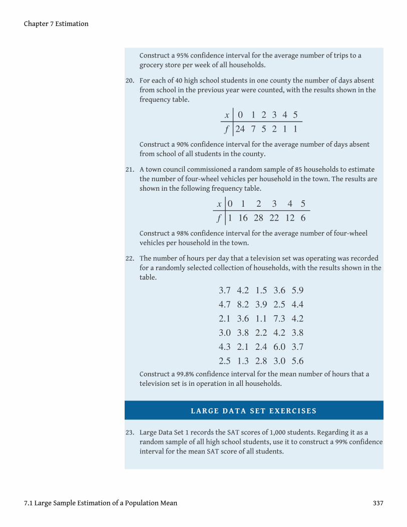
20. For each of 40 high school students in one county the number of days absentfrom school in the previous year were counted, with the results shown in thefrequency table.

Construct a 90% confidence interval for the average number of days absentfrom school of all students in the county.

21. A town council commissioned a random sample of 85 households to estimatethe number of four-wheel vehicles per household in the town. The results areshown in the following frequency table.

Construct a 98% confidence interval for the average number of four-wheelvehicles per household in the town.

22. The number of hours per day that a television set was operating was recordedfor a randomly selected collection of households, with the results shown in thetable.

Construct a 99.8% confidence interval for the mean number of hours that atelevision set is in operation in all households.

LARGE DATA SET EXERCISES

23. Large Data Set 1 records the SAT scores of 1,000 students. Regarding it as arandom sample of all high school students, use it to construct a 99% confidenceinterval for the mean SAT score of all students.

x

f

024

17

25

32

41

51

x

f

01

116

228

322

412

56

3.74.72.13.04.32.5

4.28.23.63.82.11.3

1.53.91.12.22.42.8

3.62.57.34.26.03.0

5.94.44.23.83.75.6



http://www.gone.2012books.lardbucket.org/sites/all/files/data1.xls

24. Large Data Set 1 records the GPAs of 1,000 college students. Regarding it as arandom sample of all college students, use it to construct a 95% confidenceinterval for the mean GPA of all students.


25. Large Data Set 1 lists the SAT scores of 1,000 students.


a. Regard the data as arising from a census of all students at a high school, inwhich the SAT score of every student was measured. Compute thepopulation mean μ.

b. Regard the first 36 students as a random sample and use it to construct a99% confidence for the mean μ of all 1,000 SAT scores. Does it actuallycapture the mean μ?

26. Large Data Set 1 lists the GPAs of 1,000 students.


a. Regard the data as arising from a census of all freshman at a small collegeat the end of their first academic year of college study, in which the GPA ofevery such person was measured. Compute the population mean μ.

b. Regard the first 36 students as a random sample and use it to construct a95% confidence for the mean μ of all 1,000 GPAs. Does it actually capturethe mean μ?



ANSWERS

1. a. 105.2 ± 3.10b. 105.2 ± 1.86

3. a. 17.1 ± 0.77b. 17.1 ± 0.42

5. a. 58.2 ± 0.28b. 58.2 ± 0.36c. Asking for greater confidence requires a longer interval.

7. 12.8 ± 0.209. −1.2 ± 0.05

11. 4.4 ± 0.7913. 3.7 ± 0.1915. 2785 ± 6117. 6.02 ± 0.0319. 2.8 ± 0.4821. 2.54 ± 0.30

23. (1511. 43,1546. 05)25. a. μ = 1528.74

b. (1428. 22,1602. 89)



7.2 Small Sample Estimation of a Population Mean

LEARNING OBJECTIVES

1. To become familiar with Student’s t-distribution.2. To understand how to apply additional formulas for a confidence

interval for a population mean.

The confidence interval formulas in the previous section are based on the CentralLimit Theorem, the statement that for large samples X

⎯⎯ is normally distributed with

mean μ and standard deviation σ / n⎯⎯

√ .When the population mean μ is estimated

with a small sample (n < 30), the Central Limit Theorem does not apply. In order toproceed we assume that the numerical population from which the sample is takenhas a normal distribution to begin with. If this condition is satisfied then when the

population standard deviation σ is known the old formula x⎯⎯ ± zα∕2 (σ / n⎯⎯

√ )can

still be used to construct a 100 (1 − α)% confidence interval for μ.

If the population standard deviation is unknown and the sample size n is small thenwhen we substitute the sample standard deviation s for σ the normalapproximation is no longer valid. The solution is to use a different distribution,called Student’s t-distribution4 with n−1 degrees of freedom5. Student’s t-distribution is very much like the standard normal distribution in that it is centeredat 0 and has the same qualitative bell shape, but it has heavier tails than thestandard normal distribution does, as indicated by Figure 7.5 "Student’s ", in whichthe curve (in brown) that meets the dashed vertical line at the lowest point is the t-distribution with two degrees of freedom, the next curve (in blue) is the t-distribution with five degrees of freedom, and the thin curve (in red) is the standardnormal distribution. As also indicated by the figure, as the sample size n increases,Student’s t-distribution ever more closely resembles the standard normaldistribution. Although there is a different t-distribution for every value of n, oncethe sample size is 30 or more it is typically acceptable to use the standard normaldistribution instead, as we will always do in this text.4. A distribution of a continuous

random variable thatresembles that standardnormal distribution but hasheavier tails.

5. A number that specifies aparticular t-distribution andthat is computed based on thesample size.


340

Figure 7.5 Student’s t-Distribution

Just as the symbol zc stands for the value that cuts off a right tail of area c in the

standard normal distribution, so the symbol tc stands for the value that cuts off a

right tail of area c in the standard normal distribution. This gives us the followingconfidence interval formulas.


7.2 Small Sample Estimation of a Population Mean 341

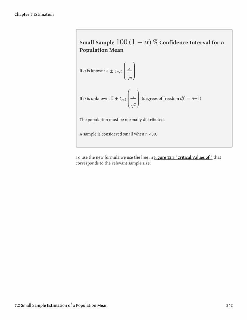
Small Sample 100 (1 − α)% Confidence Interval for aPopulation Mean

If σ is known: x⎯⎯ ± zα∕2

σ

n√

If σ is unknown: x⎯⎯ ± tα∕2

s

n√

(degrees of freedom df = n−1)

The population must be normally distributed.

A sample is considered small when n < 30.

To use the new formula we use the line in Figure 12.3 "Critical Values of " thatcorresponds to the relevant sample size.



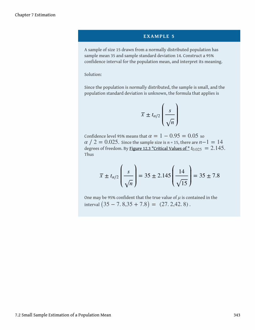
EXAMPLE 5

A sample of size 15 drawn from a normally distributed population hassample mean 35 and sample standard deviation 14. Construct a 95%confidence interval for the population mean, and interpret its meaning.

Solution:

Since the population is normally distributed, the sample is small, and thepopulation standard deviation is unknown, the formula that applies is

Confidence level 95% means that α = 1 − 0.95 = 0.05 soα ∕ 2 = 0.025. Since the sample size is n = 15, there are n−1 = 14degrees of freedom. By Figure 12.3 "Critical Values of " t0.025 = 2.145.Thus

One may be 95% confident that the true value of μ is contained in the

interval (35 − 7. 8,35 + 7.8) = (27. 2,42. 8) .

x⎯⎯ ± tα∕2

s

n⎯⎯

√

x⎯⎯ ± tα∕2

s

n⎯⎯

√

= 35 ± 2.145

14

15⎯ ⎯⎯⎯

√

= 35 ± 7.8



EXAMPLE 6

A random sample of 12 students from a large university yields mean GPA2.71 with sample standard deviation 0.51. Construct a 90% confidenceinterval for the mean GPA of all students at the university. Assume that thenumerical population of GPAs from which the sample is taken has a normaldistribution.

Solution:

Since the population is normally distributed, the sample is small, and thepopulation standard deviation is unknown, the formula that applies is

Confidence level 90% means that α = 1 − 0.90 = 0.10 soα ∕ 2 = 0.05. Since the sample size is n = 12, there are n−1 = 11degrees of freedom. By Figure 12.3 "Critical Values of " t0.05 = 1.796.Thus

One may be 90% confident that the true average GPA of all students at theuniversity is contained in the interval

(2.71 − 0. 26,2. 71 + 0.26) = (2. 45,2. 97) .

Compare Note 7.9 "Example 4" in Section 7.1 "Large Sample Estimation of aPopulation Mean" and Note 7.16 "Example 6". The summary statistics in the twosamples are the same, but the 90% confidence interval for the average GPA of allstudents at the university in Note 7.9 "Example 4" in Section 7.1 "Large SampleEstimation of a Population Mean", (2. 63,2. 79), is shorter than the 90% confidence

interval (2. 45,2. 97), in Note 7.16 "Example 6". This is partly because in Note 7.9"Example 4" the sample size is larger; there is more information pertaining to thetrue value of μ in the large data set than in the small one.

x⎯⎯ ± tα∕2

s

n⎯⎯

√

x⎯⎯ ± tα∕2

s

n⎯⎯

√

= 2.71 ± 1.796

0.51

12⎯ ⎯⎯⎯

√

= 2.71 ± 0.26



KEY TAKEAWAYS

• In selecting the correct formula for construction of a confidence intervalfor a population mean ask two questions: is the population standarddeviation σ known or unknown, and is the sample large or small?

• We can construct confidence intervals with small samples only if thepopulation is normal.



EXERCISES

BASIC

1. A random sample is drawn from a normally distributed population of knownstandard deviation 5. Construct a 99.8% confidence interval for the populationmean based on the information given (not all of the information given need beused).

a. n = 16, x⎯⎯ = 98, s = 5.6b. n = 9, x⎯⎯ = 98, s = 5.6

2. A random sample is drawn from a normally distributed population of knownstandard deviation 10.7. Construct a 95% confidence interval for thepopulation mean based on the information given (not all of the informationgiven need be used).

a. n = 25, x⎯⎯ = 103.3 , s = 11.0b. n = 4, x⎯⎯ = 103.3 , s = 11.0

3. A random sample is drawn from a normally distributed population of unknownstandard deviation. Construct a 99% confidence interval for the populationmean based on the information given.

a. n = 18, x⎯⎯ = 386, s = 24b. n = 7, x⎯⎯ = 386, s = 24

4. A random sample is drawn from a normally distributed population of unknownstandard deviation. Construct a 98% confidence interval for the populationmean based on the information given.

a. n = 8, x⎯⎯ = 58.3, s = 4.1b. n = 27, x⎯⎯ = 58.3, s = 4.1

5. A random sample of size 14 is drawn from a normal population. The summarystatistics are x⎯⎯ = 933 and s = 18.

a. Construct an 80% confidence interval for the population mean μ.b. Construct a 90% confidence interval for the population mean μ.c. Comment on why one interval is longer than the other.

6. A random sample of size 28 is drawn from a normal population. The summarystatistics are x⎯⎯ = 68.6 and s = 1.28.

a. Construct a 95% confidence interval for the population mean μ.



b. Construct a 99.5% confidence interval for the population mean μ.c. Comment on why one interval is longer than the other.

APPLICATIONS

7. City planners wish to estimate the mean lifetime of the most commonlyplanted trees in urban settings. A sample of 16 recently felled trees yieldedmean age 32.7 years with standard deviation 3.1 years. Assuming the lifetimesof all such trees are normally distributed, construct a 99.8% confidenceinterval for the mean lifetime of all such trees.

8. To estimate the number of calories in a cup of diced chicken breast meat, thenumber of calories in a sample of four separate cups of meat is measured. Thesample mean is 211.8 calories with sample standard deviation 0.9 calorie.Assuming the caloric content of all such chicken meat is normally distributed,construct a 95% confidence interval for the mean number of calories in onecup of meat.

9. A college athletic program wishes to estimate the average increase in the totalweight an athlete can lift in three different lifts after following a particulartraining program for six weeks. Twenty-five randomly selected athletes whenplaced on the program exhibited a mean gain of 47.3 lb with standarddeviation 6.4 lb. Construct a 90% confidence interval for the mean increase inlifting capacity all athletes would experience if placed on the trainingprogram. Assume increases among all athletes are normally distributed.

10. To test a new tread design with respect to stopping distance, a tiremanufacturer manufactures a set of prototype tires and measures the stoppingdistance from 70 mph on a standard test car. A sample of 25 stopping distancesyielded a sample mean 173 feet with sample standard deviation 8 feet.Construct a 98% confidence interval for the mean stopping distance for thesetires. Assume a normal distribution of stopping distances.

11. A manufacturer of chokes for shotguns tests a choke by shooting 15 patterns attargets 40 yards away with a specified load of shot. The mean number of shotin a 30-inch circle is 53.5 with standard deviation 1.6. Construct an 80%confidence interval for the mean number of shot in a 30-inch circle at 40 yardsfor this choke with the specified load. Assume a normal distribution of thenumber of shot in a 30-inch circle at 40 yards for this choke.

12. In order to estimate the speaking vocabulary of three-year-old children in aparticular socioeconomic class, a sociologist studies the speech of fourchildren. The mean and standard deviation of the sample are x⎯⎯ = 1120 ands = 215 words. Assuming that speaking vocabularies are normally distributed,



construct an 80% confidence interval for the mean speaking vocabulary of allthree-year-old children in this socioeconomic group.

13. A thread manufacturer tests a sample of eight lengths of a certain type ofthread made of blended materials and obtains a mean tensile strength of 8.2 lbwith standard deviation 0.06 lb. Assuming tensile strengths are normallydistributed, construct a 90% confidence interval for the mean tensile strengthof this thread.

14. An airline wishes to estimate the weight of the paint on a fully painted aircraftof the type it flies. In a sample of four repaintings the average weight of thepaint applied was 239 pounds, with sample standard deviation 8 pounds.Assuming that weights of paint on aircraft are normally distributed, constructa 99.8% confidence interval for the mean weight of paint on all such aircraft.

15. In a study of dummy foal syndrome, the average time between birth and onsetof noticeable symptoms in a sample of six foals was 18.6 hours, with standarddeviation 1.7 hours. Assuming that the time to onset of symptoms in all foals isnormally distributed, construct a 90% confidence interval for the mean timebetween birth and onset of noticeable symptoms.

16. A sample of 26 women’s size 6 dresses had mean waist measurement 25.25inches with sample standard deviation 0.375 inch. Construct a 95% confidenceinterval for the mean waist measurement of all size 6 women’s dresses. Assumewaist measurements are normally distributed.


17. Botanists studying attrition among saplings in new growth areas of forestsdiligently counted stems in six plots in five-year-old new growth areas,obtaining the following counts of stems per acre:

Construct an 80% confidence interval for the mean number of stems per acrein all five-year-old new growth areas of forests. Assume that the number ofstems per acre is normally distributed.

18. Nutritionists are investigating the efficacy of a diet plan designed to increasethe caloric intake of elderly people. The increase in daily caloric intake in 12individuals who are put on the plan is (a minus sign signifies that caloriesconsumed went down):

9,4328,773

11,0269,868

10,53910,247



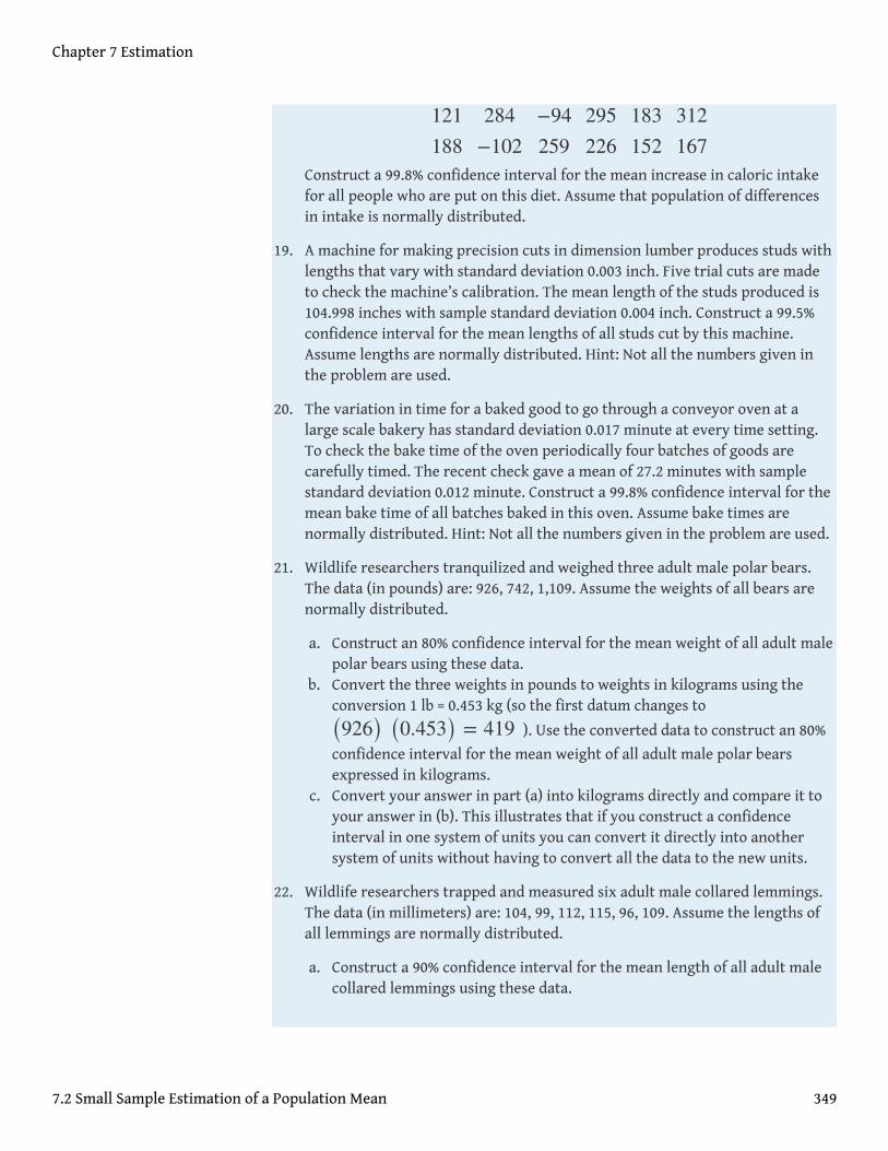
Construct a 99.8% confidence interval for the mean increase in caloric intakefor all people who are put on this diet. Assume that population of differencesin intake is normally distributed.

19. A machine for making precision cuts in dimension lumber produces studs withlengths that vary with standard deviation 0.003 inch. Five trial cuts are madeto check the machine’s calibration. The mean length of the studs produced is104.998 inches with sample standard deviation 0.004 inch. Construct a 99.5%confidence interval for the mean lengths of all studs cut by this machine.Assume lengths are normally distributed. Hint: Not all the numbers given inthe problem are used.

20. The variation in time for a baked good to go through a conveyor oven at alarge scale bakery has standard deviation 0.017 minute at every time setting.To check the bake time of the oven periodically four batches of goods arecarefully timed. The recent check gave a mean of 27.2 minutes with samplestandard deviation 0.012 minute. Construct a 99.8% confidence interval for themean bake time of all batches baked in this oven. Assume bake times arenormally distributed. Hint: Not all the numbers given in the problem are used.

21. Wildlife researchers tranquilized and weighed three adult male polar bears.The data (in pounds) are: 926, 742, 1,109. Assume the weights of all bears arenormally distributed.

a. Construct an 80% confidence interval for the mean weight of all adult malepolar bears using these data.

b. Convert the three weights in pounds to weights in kilograms using theconversion 1 lb = 0.453 kg (so the first datum changes to

(926) (0.453) = 419 ). Use the converted data to construct an 80%

confidence interval for the mean weight of all adult male polar bearsexpressed in kilograms.

c. Convert your answer in part (a) into kilograms directly and compare it toyour answer in (b). This illustrates that if you construct a confidenceinterval in one system of units you can convert it directly into anothersystem of units without having to convert all the data to the new units.

22. Wildlife researchers trapped and measured six adult male collared lemmings.The data (in millimeters) are: 104, 99, 112, 115, 96, 109. Assume the lengths ofall lemmings are normally distributed.

a. Construct a 90% confidence interval for the mean length of all adult malecollared lemmings using these data.

121188

284−102

−94259

295226

183152

312167



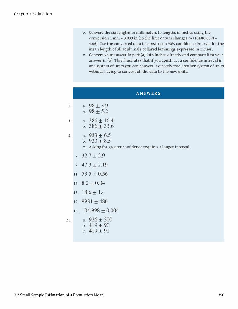
b. Convert the six lengths in millimeters to lengths in inches using theconversion 1 mm = 0.039 in (so the first datum changes to (104)(0.039) =4.06). Use the converted data to construct a 90% confidence interval for themean length of all adult male collared lemmings expressed in inches.

c. Convert your answer in part (a) into inches directly and compare it to youranswer in (b). This illustrates that if you construct a confidence interval inone system of units you can convert it directly into another system of unitswithout having to convert all the data to the new units.

ANSWERS

1. a. 98 ± 3.9b. 98 ± 5.2

3. a. 386 ± 16.4b. 386 ± 33.6

5. a. 933 ± 6.5b. 933 ± 8.5c. Asking for greater confidence requires a longer interval.

7. 32.7 ± 2.99. 47.3 ± 2.19

11. 53.5 ± 0.5613. 8.2 ± 0.0415. 18.6 ± 1.417. 9981 ± 48619. 104.998 ± 0.004

21. a. 926 ± 200b. 419 ± 90c. 419 ± 91



7.3 Large Sample Estimation of a Population Proportion

LEARNING OBJECTIVE

1. To understand how to apply the formula for a confidence interval for apopulation proportion.

Since from Section 6.3 "The Sample Proportion" in Chapter 6 "SamplingDistributions" we know the mean, standard deviation, and sampling distribution ofthe sample proportion p, the ideas of the previous two sections can be applied toproduce a confidence interval for a population proportion. Here is the formula.

Large Sample 100 (1 − α)% Confidence Interval for aPopulation Proportion

A sample is large if the interval [p−3 σP, p + 3 σ

P] lies wholly within the

interval [0,1] .

In actual practice the value of p is not known, hence neither is σP. In that case we

substitute the known quantity p for p in making the check; this means checkingthat the interval

lies wholly within the interval [0,1] .

p ± zα∕2p (1 − p)

n

⎯ ⎯⎯⎯⎯⎯⎯⎯⎯⎯⎯⎯⎯⎯⎯⎯

√

p−3

p (1 − p)n

⎯ ⎯⎯⎯⎯⎯⎯⎯⎯⎯⎯⎯⎯⎯⎯⎯

√ , p + 3p (1 − p)

n

⎯ ⎯⎯⎯⎯⎯⎯⎯⎯⎯⎯⎯⎯⎯⎯⎯

√


351

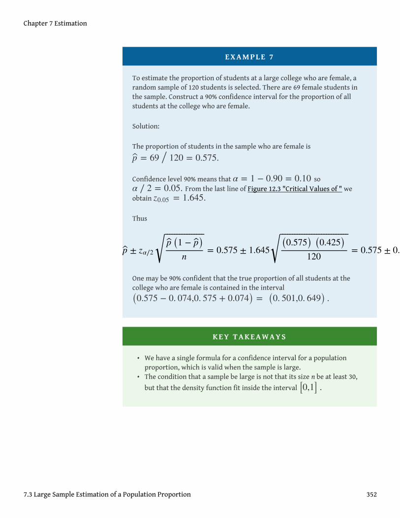
EXAMPLE 7

To estimate the proportion of students at a large college who are female, arandom sample of 120 students is selected. There are 69 female students inthe sample. Construct a 90% confidence interval for the proportion of allstudents at the college who are female.

Solution:

The proportion of students in the sample who are female is

p = 69 / 120 = 0.575.

Confidence level 90% means that α = 1 − 0.90 = 0.10 soα ∕ 2 = 0.05. From the last line of Figure 12.3 "Critical Values of " weobtain z0.05 = 1.645.

Thus

One may be 90% confident that the true proportion of all students at thecollege who are female is contained in the interval

(0.575 − 0. 074,0. 575 + 0.074) = (0. 501,0. 649) .

KEY TAKEAWAYS

• We have a single formula for a confidence interval for a populationproportion, which is valid when the sample is large.

• The condition that a sample be large is not that its size n be at least 30,

but that the density function fit inside the interval [0,1] .

p ± zα∕2p (1 − p)

n

⎯ ⎯⎯⎯⎯⎯⎯⎯⎯⎯⎯⎯⎯⎯⎯⎯

√ = 0.575 ± 1.645 (0.575) (0.425)120

⎯ ⎯⎯⎯⎯⎯⎯⎯⎯⎯⎯⎯⎯⎯⎯⎯⎯⎯⎯⎯⎯⎯⎯⎯⎯⎯⎯⎯

√ = 0.575 ± 0.074


7.3 Large Sample Estimation of a Population Proportion 352

EXERCISES

BASIC

1. Information about a random sample is given. Verify that the sample is largeenough to use it to construct a confidence interval for the populationproportion. Then construct a 90% confidence interval for the populationproportion.

a. n = 25, p = 0.7b. n = 50, p = 0.7


a. n = 2500, p = 0.22b. n = 1200, p = 0.22


a. n = 80, p = 0.4b. n = 325, p = 0.4

4. Information about a random sample is given. Verify that the sample is largeenough to use it to construct a confidence interval for the populationproportion. Then construct a 99.5% confidence interval for the populationproportion.

a. n = 200, p = 0.85b. n = 75, p = 0.85

5. In a random sample of size 1,100, 338 have the characteristic of interest.

a. Compute the sample proportion p with the characteristic of interest.b. Verify that the sample is large enough to use it to construct a confidence

interval for the population proportion.c. Construct an 80% confidence interval for the population proportion p.d. Construct a 90% confidence interval for the population proportion p.e. Comment on why one interval is longer than the other.



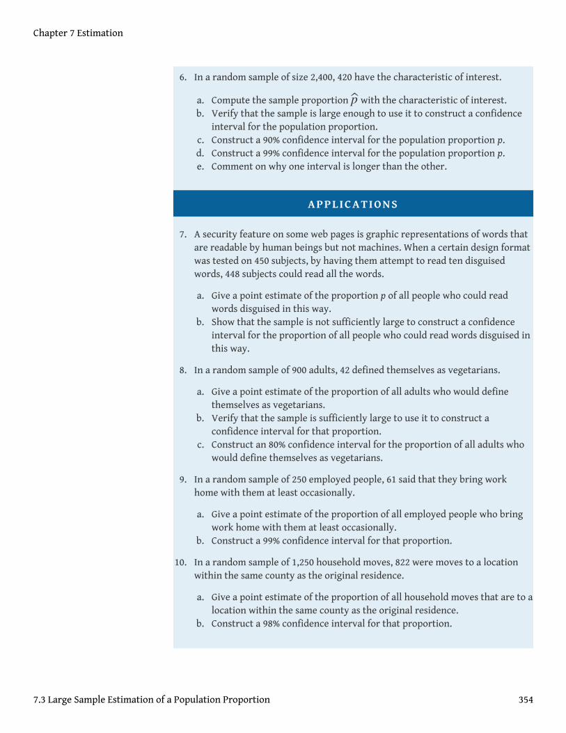
6. In a random sample of size 2,400, 420 have the characteristic of interest.

a. Compute the sample proportion p with the characteristic of interest.b. Verify that the sample is large enough to use it to construct a confidence

interval for the population proportion.c. Construct a 90% confidence interval for the population proportion p.d. Construct a 99% confidence interval for the population proportion p.e. Comment on why one interval is longer than the other.

APPLICATIONS

7. A security feature on some web pages is graphic representations of words thatare readable by human beings but not machines. When a certain design formatwas tested on 450 subjects, by having them attempt to read ten disguisedwords, 448 subjects could read all the words.

a. Give a point estimate of the proportion p of all people who could readwords disguised in this way.

b. Show that the sample is not sufficiently large to construct a confidenceinterval for the proportion of all people who could read words disguised inthis way.

8. In a random sample of 900 adults, 42 defined themselves as vegetarians.

a. Give a point estimate of the proportion of all adults who would definethemselves as vegetarians.

b. Verify that the sample is sufficiently large to use it to construct aconfidence interval for that proportion.

c. Construct an 80% confidence interval for the proportion of all adults whowould define themselves as vegetarians.

9. In a random sample of 250 employed people, 61 said that they bring workhome with them at least occasionally.

a. Give a point estimate of the proportion of all employed people who bringwork home with them at least occasionally.

b. Construct a 99% confidence interval for that proportion.

10. In a random sample of 1,250 household moves, 822 were moves to a locationwithin the same county as the original residence.

a. Give a point estimate of the proportion of all household moves that are to alocation within the same county as the original residence.

b. Construct a 98% confidence interval for that proportion.



11. In a random sample of 12,447 hip replacement or revision surgery proceduresnationwide, 162 patients developed a surgical site infection.

a. Give a point estimate of the proportion of all patients undergoing a hipsurgery procedure who develop a surgical site infection.


c. Construct a 95% confidence interval for the proportion of all patientsundergoing a hip surgery procedure who develop a surgical site infection.

12. In a certain region prepackaged products labeled 500 g must contain onaverage at least 500 grams of the product, and at least 90% of all packages mustweigh at least 490 grams. In a random sample of 300 packages, 288 weighed atleast 490 grams.

a. Give a point estimate of the proportion of all packages that weigh at least490 grams.


c. Construct a 99.8% confidence interval for the proportion of all packagesthat weigh at least 490 grams.

13. A survey of 50 randomly selected adults in a small town asked them if theiropinion on a proposed “no cruising” restriction late at night. Responses werecoded 1 for in favor, 0 for indifferent, and 2 for opposed, with the resultsshown in the table.

a. Give a point estimate of the proportion of all adults in the community whoare indifferent concerning the proposed restriction.

b. Assuming that the sample is sufficiently large, construct a 90% confidenceinterval for the proportion of all adults in the community who areindifferent concerning the proposed restriction.

14. To try to understand the reason for returned goods, the manager of a storeexamines the records on 40 products that were returned in the last year.Reasons were coded by 1 for “defective,” 2 for “unsatisfactory,” and 0 for allother reasons, with the results shown in the table.

10001

02220

20100

00221

10002

01010

00000

12202

10021

20102



a. Give a point estimate of the proportion of all returns that are because ofsomething wrong with the product, that is, either defective or performedunsatisfactorily.

b. Assuming that the sample is sufficiently large, construct an 80%confidence interval for the proportion of all returns that are because ofsomething wrong with the product.

15. In order to estimate the proportion of entering students who graduate withinsix years, the administration at a state university examined the records of 600randomly selected students who entered the university six years ago, andfound that 312 had graduated.

a. Give a point estimate of the six-year graduation rate, the proportion ofentering students who graduate within six years.

b. Assuming that the sample is sufficiently large, construct a 98% confidenceinterval for the six-year graduation rate.

16. In a random sample of 2,300 mortgages taken out in a certain region last year,187 were adjustable-rate mortgages.

a. Give a point estimate of the proportion of all mortgages taken out in thisregion last year that were adjustable-rate mortgages.

b. Assuming that the sample is sufficiently large, construct a 99.9%confidence interval for the proportion of all mortgages taken out in thisregion last year that were adjustable-rate mortgages.

17. In a research study in cattle breeding, 159 of 273 cows in several herds thatwere in estrus were detected by means of an intensive once a day, one-hourobservation of the herds in early morning.

a. Give a point estimate of the proportion of all cattle in estrus who aredetected by this method.

b. Assuming that the sample is sufficiently large, construct a 90% confidenceinterval for the proportion of all cattle in estrus who are detected by thismethod.

18. A survey of 21,250 households concerning telephone service gave the resultsshown in the table.

0000

2000

0020

0000

0000

0001

0000

2020

0000

0200



Landline No Landline

Cell phone 12,474 5,844

No cell phone 2,529 403

a. Give a point estimate for the proportion of all households in which there isa cell phone but no landline.

b. Assuming the sample is sufficiently large, construct a 99.9% confidenceinterval for the proportion of all households in which there is a cell phonebut no landline.

c. Give a point estimate for the proportion of all households in which there isno telephone service of either kind.

d. Assuming the sample is sufficiently large, construct a 99.9% confidenceinterval for the proportion of all all households in which there is notelephone service of either kind.


19. In a random sample of 900 adults, 42 defined themselves as vegetarians. Ofthese 42, 29 were women.

a. Give a point estimate of the proportion of all self-described vegetarianswho are women.


c. Construct a 90% confidence interval for the proportion of all all self-described vegetarians who are women.

20. A random sample of 185 college soccer players who had suffered injuries thatresulted in loss of playing time was made with the results shown in the table.Injuries are classified according to severity of the injury and the conditionunder which it was sustained.

Minor Moderate Serious

Practice 48 20 6

Game 62 32 17

a. Give a point estimate for the proportion p of all injuries to college soccerplayers that are sustained in practice.

b. Construct a 95% confidence interval for the proportion p of all injuries tocollege soccer players that are sustained in practice.

c. Give a point estimate for the proportion p of all injuries to college soccerplayers that are either moderate or serious.



d. Construct a 95% confidence interval for the proportion p of all injuries tocollege soccer players that are either moderate or serious.

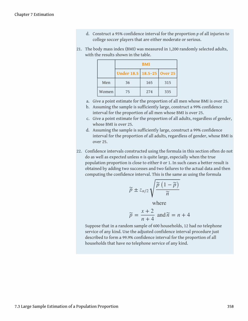
21. The body mass index (BMI) was measured in 1,200 randomly selected adults,with the results shown in the table.

BMI

Under 18.5 18.5–25 Over 25

Men 36 165 315

Women 75 274 335

a. Give a point estimate for the proportion of all men whose BMI is over 25.b. Assuming the sample is sufficiently large, construct a 99% confidence

interval for the proportion of all men whose BMI is over 25.c. Give a point estimate for the proportion of all adults, regardless of gender,

whose BMI is over 25.d. Assuming the sample is sufficiently large, construct a 99% confidence

interval for the proportion of all adults, regardless of gender, whose BMI isover 25.

22. Confidence intervals constructed using the formula in this section often do notdo as well as expected unless n is quite large, especially when the truepopulation proportion is close to either 0 or 1. In such cases a better result isobtained by adding two successes and two failures to the actual data and thencomputing the confidence interval. This is the same as using the formula

Suppose that in a random sample of 600 households, 12 had no telephoneservice of any kind. Use the adjusted confidence interval procedure justdescribed to form a 99.9% confidence interval for the proportion of allhouseholds that have no telephone service of any kind.

p ± zα∕2p (1 − p)

n

⎯ ⎯⎯⎯⎯⎯⎯⎯⎯⎯⎯⎯⎯⎯⎯⎯

√where

p =x + 2n + 4

and n = n + 4



LARGE DATA SET EXERCISES

23. Large Data Sets 4 and 4A list the results of 500 tosses of a die. Let p denote theproportion of all tosses of this die that would result in a four. Use the sampledata to construct a 90% confidence interval for p.


http://www.gone.2012books.lardbucket.org/sites/all/files/data4A.xls

24. Large Data Set 6 records results of a random survey of 200 voters in each of tworegions, in which they were asked to express whether they prefer Candidate Afor a U.S. Senate seat or prefer some other candidate. Use the full data set (400observations) to construct a 98% confidence interval for the proportion p of allvoters who prefer Candidate A.


25. Lines 2 through 536 in Large Data Set 11 is a sample of 535 real estate sales in acertain region in 2008. Those that were foreclosure sales are identified with a 1in the second column.


a. Use these data to construct a point estimate p of the proportion p of allreal estate sales in this region in 2008 that were foreclosure sales.

b. Use these data to construct a 90% confidence for p.

26. Lines 537 through 1106 in Large Data Set 11 is a sample of 570 real estate salesin a certain region in 2010. Those that were foreclosure sales are identifiedwith a 1 in the second column.


a. Use these data to construct a point estimate p of the proportion p of allreal estate sales in this region in 2010 that were foreclosure sales.

b. Use these data to construct a 90% confidence for p.



ANSWERS

1. a. (0.5492, 0.8508)b. (0.5934, 0.8066)

3. a. (0.2726, 0.5274)b. (0.3368, 0.4632)

5. a. 0.3073

b. p ± 3 pqn

⎯ ⎯⎯⎯⎯√ = 0.31 ± 0.04

and

[0. 27,0. 35] ⊂ [0,1]c. (0.2895, 0.3251)d. (0.2844, 0.3302)e. Asking for greater confidence requires a longer interval.

7. a. 0.9956b. (0.9862, 1.005)

9. a. 0.244b. (0.1740, 0.3140)

11. a. 0.013b. (0.01, 0.016)c. (0.011, 0.015)

13. a. 0.52b. (0.4038, 0.6362)

15. a. 0.52b. (0.4726, 0.5674)

17. a. 0.5824b. (0.5333, 0.6315)

19. a. 0.69

b. p ± 3 pqn

⎯ ⎯⎯⎯⎯√ = 0.69 ± 0.21

and

[0. 48,0. 90] ⊂ [0,1]c. 0.69 ± 0.12



21. a. 0.6105b. (0.5552, 0.6658)c. 0.5583d. (0.5214, 0.5952)

23. (0. 1368,0. 1912)25. a. p = 0.2280

b. (0. 1982,0. 2579)



7.4 Sample Size Considerations

LEARNING OBJECTIVE

1. To learn how to apply formulas for estimating the size sample that willbe needed in order to construct a confidence interval for a populationmean or proportion that meets given criteria.

Sampling is typically done with a set of clear objectives in mind. For example, aneconomist might wish to estimate the mean yearly income of workers in aparticular industry at 90% confidence and to within $500. Since sampling costs time,effort, and money, it would be useful to be able to estimate the smallest size samplethat is likely to meet these criteria.

Estimating μ

The confidence interval formulas for estimating a population mean μ have the formx⎯⎯ ± E.When the population standard deviation σ is known,

The number zα∕2 is determined by the desired level of confidence. To say that wewish to estimate the mean to within a certain number of units means that we wantthe margin of error E to be no larger than that number. Thus we obtain theminimum sample size needed by solving the displayed equation for n.

Minimum Sample Size for Estimating a Population Mean

The estimated minimum sample size n needed to estimate a population mean μto within E units at 100 (1 − α)% confidence is

E =zα∕2σ

n⎯⎯

√

n = (zα∕2)2σ 2

E2 (rounded up)


362

To apply the formula we must have prior knowledge of the population in order tohave an estimate of its standard deviation σ. In all the examples and exercises thepopulation standard deviation will be given.

EXAMPLE 8

Find the minimum sample size necessary to construct a 99% confidenceinterval for μ with a margin of error E = 0.2. Assume that the populationstandard deviation is σ = 1.3.

Solution:

Confidence level 99% means that α = 1 − 0.99 = 0.01 soα ∕ 2 = 0.005. From the last line of Figure 12.3 "Critical Values of " weobtain z0.005 = 2.576. Thus

which we round up to 281, since it is impossible to take a fractionalobservation.

n = (zα∕2)2σ 2

E2 = (2.576)2 (1.3)2

(0.2)2= 280.361536


7.4 Sample Size Considerations 363

EXAMPLE 9

An economist wishes to estimate, with a 95% confidence interval, the yearlyincome of welders with at least five years experience to within $1,000. Heestimates that the range of incomes is no more than $24,000, so using theEmpirical Rule he estimates the population standard deviation to be aboutone-sixth as much, or about $4,000. Find the estimated minimum samplesize required.

Solution:


To say that the estimate is to be “to within $1,000” means that E = 1000. Thus

which we round up to 62.

Estimating p

The confidence interval formula for estimating a population proportion p is p ± E,where

The number zα∕2 is determined by the desired level of confidence. To say that wewish to estimate the population proportion to within a certain number ofpercentage points means that we want the margin of error E to be no larger thanthat number (expressed as a proportion). Thus we obtain the minimum sample sizeneeded by solving the displayed equation for n.

n = (zα∕2)2σ 2

E2 = (1.960)2 (4000) 2

(1000) 2= 61.4656

E = zα∕2p (1 − p)

n

⎯ ⎯⎯⎯⎯⎯⎯⎯⎯⎯⎯⎯⎯⎯⎯⎯

√



Minimum Sample Size for Estimating a PopulationProportion

The estimated minimum sample size n needed to estimate a populationproportion p to within E at 100 (1 − α)% confidence is

There is a dilemma here: the formula for estimating how large a sample to takecontains the number p, which we know only after we have taken the sample. Thereare two ways out of this dilemma. Typically the researcher will have some idea as tothe value of the population proportion p, hence of what the sample proportion p islikely to be. For example, if last month 37% of all voters thought that state taxes aretoo high, then it is likely that the proportion with that opinion this month will notbe dramatically different, and we would use the value 0.37 for p in the formula.

The second approach to resolving the dilemma is simply to replace p in the formulaby 0.5. This is because if p is large then 1 − p is small, and vice versa, which limitstheir product to a maximum value of 0.25, which occurs when p = 0.5. This iscalled the most conservative estimate6, since it gives the largest possible estimateof n.

n = (zα∕2)2p (1 − p)E2 (rounded up)

6. The estimate obtained usingp = 0.5, which gives thelargest estimate of n.



EXAMPLE 10

Find the necessary minimum sample size to construct a 98% confidenceinterval for p with a margin of error E = 0.05,

a. assuming that no prior knowledge about p is available; andb. assuming that prior studies suggest that p is about 0.1.

Solution:


a. Since there is no prior knowledge of p we make the most

conservative estimate that p = 0.5. Then


b. Since p ≈ 0.1 we estimate p by 0.1, and obtain


n = (zα∕2)2p (1 − p)E2 = (2.326)

2 (0.5) (1 − 0.5)0.052 = 541.0276

n = (zα∕2)2p (1 − p)E2 = (2.326)

2 (0.1) (1 − 0.1)

0.052 = 194.769936



EXAMPLE 11

A dermatologist wishes to estimate the proportion of young adults whoapply sunscreen regularly before going out in the sun in the summer. Findthe minimum sample size required to estimate the proportion to withinthree percentage points, at 90% confidence.

Solution:


Since there is no prior knowledge of p we make the most conservative

estimate that p = 0.5. To estimate “to within three percentage points”means that E = 0.03. Then


KEY TAKEAWAYS

• If the population standard deviation σ is known or can be estimated,then the minimum sample size needed to obtain a confidence intervalfor the population mean with a given maximum error of the estimateand a given level of confidence can be estimated.

• The minimum sample size needed to obtain a confidence interval for apopulation proportion with a given maximum error of the estimate anda given level of confidence can always be estimated. If there is priorknowledge of the population proportion p then the estimate can besharpened.

n = (zα∕2)2p (1 − p)E2 = (1.645)

2 (0.5) (1 − 0.5)0.032 = 751.6736111



EXERCISES

BASIC

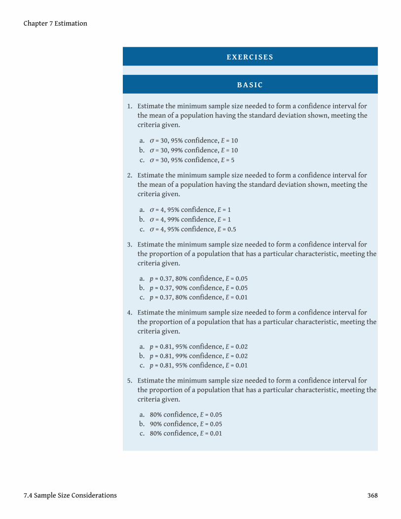
1. Estimate the minimum sample size needed to form a confidence interval forthe mean of a population having the standard deviation shown, meeting thecriteria given.

a. σ = 30, 95% confidence, E = 10b. σ = 30, 99% confidence, E = 10c. σ = 30, 95% confidence, E = 5

2. Estimate the minimum sample size needed to form a confidence interval forthe mean of a population having the standard deviation shown, meeting thecriteria given.

a. σ = 4, 95% confidence, E = 1b. σ = 4, 99% confidence, E = 1c. σ = 4, 95% confidence, E = 0.5

3. Estimate the minimum sample size needed to form a confidence interval forthe proportion of a population that has a particular characteristic, meeting thecriteria given.

a. p ≈ 0.37, 80% confidence, E = 0.05b. p ≈ 0.37, 90% confidence, E = 0.05c. p ≈ 0.37, 80% confidence, E = 0.01


a. p ≈ 0.81, 95% confidence, E = 0.02b. p ≈ 0.81, 99% confidence, E = 0.02c. p ≈ 0.81, 95% confidence, E = 0.01


a. 80% confidence, E = 0.05b. 90% confidence, E = 0.05c. 80% confidence, E = 0.01




a. 95% confidence, E = 0.02b. 99% confidence, E = 0.02c. 95% confidence, E = 0.01

APPLICATIONS

7. A software engineer wishes to estimate, to within 5 seconds, the mean timethat a new application takes to start up, with 95% confidence. Estimate theminimum size sample required if the standard deviation of start up times forsimilar software is 12 seconds.

8. A real estate agent wishes to estimate, to within $2.50, the mean retail cost persquare foot of newly built homes, with 80% confidence. He estimates thestandard deviation of such costs at $5.00. Estimate the minimum size samplerequired.

9. An economist wishes to estimate, to within 2 minutes, the mean time thatemployed persons spend commuting each day, with 95% confidence. On theassumption that the standard deviation of commuting times is 8 minutes,estimate the minimum size sample required.

10. A motor club wishes to estimate, to within 1 cent, the mean price of 1 gallon ofregular gasoline in a certain region, with 98% confidence. Historically thevariability of prices is measured by σ = $0.03. Estimate the minimum sizesample required.

11. A bank wishes to estimate, to within $25, the mean average monthly balance inits checking accounts, with 99.8% confidence. Assuming σ = $250 , estimatethe minimum size sample required.

12. A retailer wishes to estimate, to within 15 seconds, the mean duration oftelephone orders taken at its call center, with 99.5% confidence. In the past thestandard deviation of call length has been about 1.25 minutes. Estimate theminimum size sample required. (Be careful to express all the information inthe same units.)

13. The administration at a college wishes to estimate, to within two percentagepoints, the proportion of all its entering freshmen who graduate within fouryears, with 90% confidence. Estimate the minimum size sample required.



14. A chain of automotive repair stores wishes to estimate, to within fivepercentage points, the proportion of all passenger vehicles in operation thatare at least five years old, with 98% confidence. Estimate the minimum sizesample required.

15. An internet service provider wishes to estimate, to within one percentagepoint, the current proportion of all email that is spam, with 99.9% confidence.Last year the proportion that was spam was 71%. Estimate the minimum sizesample required.

16. An agronomist wishes to estimate, to within one percentage point, theproportion of a new variety of seed that will germinate when planted, with 95%confidence. A typical germination rate is 97%. Estimate the minimum sizesample required.

17. A charitable organization wishes to estimate, to within half a percentage point,the proportion of all telephone solicitations to its donors that result in a gift,with 90% confidence. Estimate the minimum sample size required, using theinformation that in the past the response rate has been about 30%.

18. A government agency wishes to estimate the proportion of drivers aged 16–24who have been involved in a traffic accident in the last year. It wishes to makethe estimate to within one percentage point and at 90% confidence. Find theminimum sample size required, using the information that several years agothe proportion was 0.12.


19. An economist wishes to estimate, to within six months, the mean time betweensales of existing homes, with 95% confidence. Estimate the minimum sizesample required. In his experience virtually all houses are re-sold within 40months, so using the Empirical Rule he will estimate σ by one-sixth the range,or 40 ∕ 6 = 6.7.

20. A wildlife manager wishes to estimate the mean length of fish in a large lake,to within one inch, with 80% confidence. Estimate the minimum size samplerequired. In his experience virtually no fish caught in the lake is over 23 incheslong, so using the Empirical Rule he will estimate σ by one-sixth the range, or23 ∕ 6 = 3.8.

21. You wish to estimate the current mean birth weight of all newborns in acertain region, to within 1 ounce (1/16 pound) and with 95% confidence. Asample will cost $400 plus $1.50 for every newborn weighed. You believe the



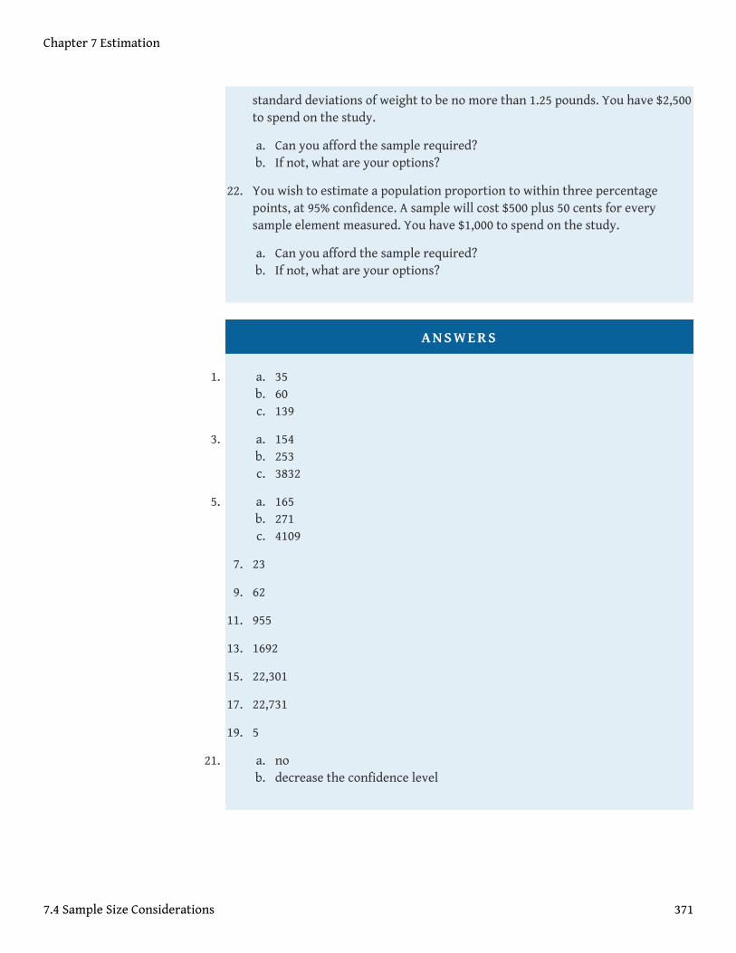
standard deviations of weight to be no more than 1.25 pounds. You have $2,500to spend on the study.

a. Can you afford the sample required?b. If not, what are your options?

22. You wish to estimate a population proportion to within three percentagepoints, at 95% confidence. A sample will cost $500 plus 50 cents for everysample element measured. You have $1,000 to spend on the study.

a. Can you afford the sample required?b. If not, what are your options?

ANSWERS

1. a. 35b. 60c. 139

3. a. 154b. 253c. 3832

5. a. 165b. 271c. 4109

7. 23

9. 62

11. 955

13. 1692

15. 22,301

17. 22,731

19. 5

21. a. nob. decrease the confidence level



chapter 7 estimation - mmathematics€¦ · the standard normal distribution"inchapter 5...

Documents