chapter 61 chapter 6 chapter 6 graphs all the programs in this file are selected from ellis...
TRANSCRIPT

CHAPTER 6 1
CHAPTER 6CHAPTER 6GRAPHS
All the programs in this file are selected from
Ellis Horowitz, Sartaj Sahni, and Susan Anderson-Freed“Fundamentals of Data Structures in C”,Computer Science Press, 1992.

CHAPTER 6 2
Definition A graph, G=(V, E), consists of two sets:
a finite set of vertices(V), and a finite, possibly empty set of edges(E) V(G) and E(G) represent the sets of vertices and edges of
G, respectively Undirected graph
The pairs of vertices representing any edges is unordered e.g., (v0, v1) and (v1, v0) represent the same edge
Directed graph Each edge as a directed pair of vertices e.g. <v0, v1> represents an edge, v0 is the tail and v1 is the
head
(v0, v1) = (v1,v0)
<v0, v1> != <v1,v0>

CHAPTER 6 3
Examples for Graph0
1 2
3
0
1
2
0
1 2
3 4 5 6G1
G2G3
V(G1)={0,1,2,3} E(G1)={(0,1),(0,2),(0,3),(1,2),(1,3),(2,3)}V(G2)={0,1,2,3,4,5,6} E(G2)={(0,1),(0,2),(1,3),(1,4),(2,5),(2,6)}V(G3)={0,1,2} E(G3)={<0,1>,<1,0>,<1,2>}
complete undirected graph: n(n-1)/2 edgescomplete directed graph: n(n-1) edges
complete graph incomplete graph

CHAPTER 6 4
Complete Graph
A complete graph is a graph that has the maximum number of edges for undirected graph with n vertices, the
maximum number of edges is n(n-1)/2 for directed graph with n vertices, the maximum
number of edges is n(n-1) example: G1 is a complete graph

CHAPTER 6 5
Adjacent and Incident
If (v0, v1) is an edge in an undirected graph, v0 and v1 are adjacent The edge (v0, v1) is incident on vertices v0 and v1
If <v0, v1> is an edge in a directed graph v0 is adjacent to v1, and v1 is adjacent from v0
The edge <v0, v1> is incident on v0 and v1

CHAPTER 6 6
0 2
1
(a)
2
1
0
3
(b)
*Figure 6.3:Example of a graph with feedback loops and a multigraph (p.260)
self edge multigraph:multiple occurrencesof the same edge
Figure 6.3

CHAPTER 6 7
A subgraph of G is a graph G’ such that V(G’) is a subset of V(G) and E(G’) is a subset of E(G)
A path from vertex vp to vertex vq in a graph G, is a sequence of vertices, vp, vi1, vi2, ..., vin, vq, such that (vp, vi1), (vi1, vi2), ..., (vin, vq) are edges in an undirected graph
The length of a path is the number of edges on it
Subgraph and Path

CHAPTER 6 8
0 0
1 2 3
1 2 0
1 2
3 (i) (ii) (iii) (iv) (a) Some of the subgraph of G1
0 0
1
0
1
2
0
1
2(i) (ii) (iii) (iv)
(b) Some of the subgraph of G3
分開單一
0
1 2
3
G1
0
1
2
G3
Figure 6.4: subgraphs of G1 and G3 (p.261)

CHAPTER 6 9
A simple path is a path in which all vertices, except possibly the first and the last, are distinct
A cycle is a simple path in which the first and the last vertices are the same
In an undirected graph G, two vertices, v0 and v1, are connected if there is a path in G from v0 to v1
An undirected graph is connected if, for every pair of distinct vertices vi, vj, there is a path from vi to vj
Simple Path and Style

CHAPTER 6 10
0
1 2
3
0
1 2
3 4 5 6G1
G2
connected
tree (acyclic graph)

CHAPTER 6 11
A connected component of an undirected graph is a maximal connected subgraph.
A tree is a graph that is connected and acyclic. A directed graph is strongly connected if there
is a directed path from vi to vj and also from vj to vi.
A strongly connected component is a maximal subgraph that is strongly connected.
Connected Component

CHAPTER 6 12
*Figure 6.5: A graph with two connected components (p.262)
1
0
2
3
4
5
6
7
H1 H2
G4 (not connected)
connected component (maximal connected subgraph)

CHAPTER 6 13
*Figure 6.6: Strongly connected components of G3 (p.262)
0
1
20
1
2
G3
not strongly connectedstrongly connected component
(maximal strongly connected subgraph)

CHAPTER 6 14
Degree The degree of a vertex is the number of edges incid
ent to that vertex For directed graph,
the in-degree of a vertex v is the number of edgesthat have v as the head
the out-degree of a vertex v is the number of edgesthat have v as the tail
if di is the degree of a vertex i in a graph G with n vertices and e edges, the number of edges is
e di
n
( ) /0
1
2

CHAPTER 6 15
undirected graph
degree0
1 2
3 4 5 6
G1 G2
3
2
3 3
1 1 1 1
directed graphin-degreeout-degree
0
1
2
G3
in:1, out: 1
in: 1, out: 2
in: 1, out: 0
0
1 2
3
33
3

CHAPTER 6 16
ADT for Graphstructure Graph is objects: a nonempty set of vertices and a set of undirected edges, where each
edge is a pair of vertices
functions: for all graph Graph, v, v1 and v2 Vertices Graph Create()::=return an empty graph Graph InsertVertex(graph, v)::= return a graph with v inserted. v has no
incident edge. Graph InsertEdge(graph, v1,v2)::= return a graph with new edge
between v1 and v2 Graph DeleteVertex(graph, v)::= return a graph in which v and all edges
incident to it are removed Graph DeleteEdge(graph, v1, v2)::=return a graph in which the edge (v1, v2)
is removed Boolean IsEmpty(graph)::= if (graph==empty graph) return TRUE else return FALSE List Adjacent(graph,v)::= return a list of all vertices that are adjacent to v

CHAPTER 6 17
常見的表示法
Adjacency matricesAdjacency listsAdjacency multilists
0
1 2
3
G1
2
1
0
G3
0
12
3
4
65
7
G4

CHAPTER 6 18
Adjacency Matrix Let G=(V,E) be a graph with n vertices. The adjacency matrix of G is a two-dimensional
n by n array, say adj_mat If the edge (vi, vj) is in E(G), adj_mat[i][j]=1 If there is no such edge in E(G), adj_mat[i][j]=0 The adjacency matrix for an undirected graph is sy
mmetric; the adjacency matrix for a digraph need not be symmetric If the matrix is sparse ?
大部分元素是 0e << (n^2/2)

CHAPTER 6 19
Examples for Adjacency Matrix
0
1
1
1
1
0
1
1
1
1
0
1
1
1
1
0
0
1
0
1
0
0
0
1
0
0
1
1
0
0
0
0
0
1
0
0
1
0
0
0
0
1
0
0
1
0
0
0
0
0
1
1
0
0
0
0
0
0
0
0
0
0
1
0
0
0
0
0
0
1
0
1
0
0
0
0
0
0
1
0
1
0
0
0
0
0
0
1
0
G1G2
G4
0
1 2
3
0
1
2
1
0
2
3
4
5
6
7
symmetric
undirected: n2/2directed: n2

CHAPTER 6 20
Merits of Adjacency Matrix
From the adjacency matrix, to determine the connection of vertices is easy
The degree of a vertex is For a digraph, the row sum is the
out_degree, while the column sum is the in_degree
adj mat i jj
n
_ [ ][ ]
0
1
ind vi A j ij
n
( ) [ , ]
0
1outd vi A i j
j
n
( ) [ , ]
0
1
CHAPTER 6 21
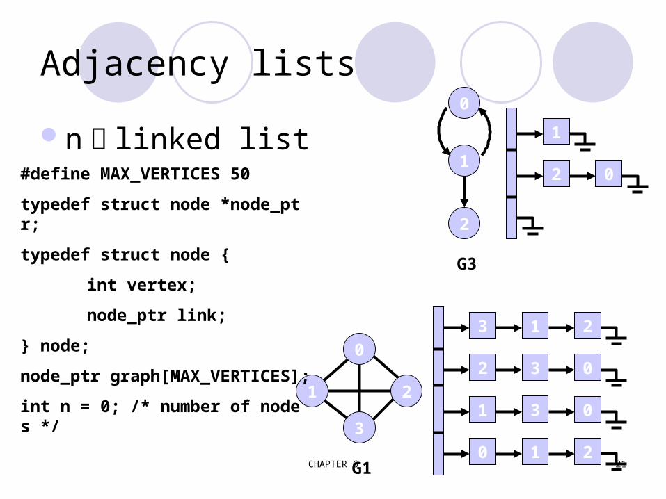
Adjacency lists
n 個 linked list 1
2 0
3 1 2
2 3 0
1 3 0
210
2
1
0
G3
0
1 2
3
G1
#define MAX_VERTICES 50
typedef struct node *node_ptr;
typedef struct node {
int vertex;
node_ptr link;
} node;
node_ptr graph[MAX_VERTICES];
int n = 0; /* number of nodes */

CHAPTER 6 22
Adjacency lists, by array
000
101
010
2
1
0
G3
1
2 0
0217754
6543210

CHAPTER 6 23
Interesting Operations
degree of a vertex in an undirected graph–# of nodes in adjacency list
# of edges in a graph–determined in O(n+e)
out-degree of a vertex in a directed graph–# of nodes in its adjacency list
in-degree of a vertex in a directed graph–traverse the whole data structure

CHAPTER 6 24
[0] 9 [8] 23 [16] 2[1] 11 [9] 1 [17] 5[2] 13 [10] 2 [18] 4[3] 15 [11] 0 [19] 6[4] 17 [12] 3 [20] 5[5] 18 [13] 0 [21] 7[6] 20 [14] 3 [22] 6[7] 22 [15] 1
1
0
2
3
4
5
6
7
0
1
2
3
45
6
7
node[0] … node[n-1]: starting point for verticesnode[n]: n+2e+1node[n+1] … node[n+2e]: head node of edge
Compact Representation

CHAPTER 6 25
tail head column link for head row link for tail
Figure 6.11: Alternate node structure for adjacency lists (p.267)

CHAPTER 6 26
0 1 2
2 NULL
1
0
1 0 NULL
0 1 NULL NULL
1 2 NULL NULL
0
1
2
0
1
0
1
0
0
0
1
0
Figure 6.12: Orthogonal representation for graph G3(p.268)

CHAPTER 6 27
Adjacency multilists
m vertex1 vertex2 list1 list2
0 2 N2 N3
N1
0 3 NIL N4
N2
1 2 N4 N5
N3
1 3 NIL N5
N4
2 3 NIL NILN5
0 1 N1 N3
N0
0
1 2
3
G1
typedef struct edge *edge_ptr;Typedef struct edge {
int marked;int vertex1;int vertex2;edge_ptr path1;edge_ptr path2;
} edge;edge_ptr graph[MAX_VERTICES];

CHAPTER 6 28
Some Graph Operations
TraversalGiven G=(V,E) and vertex v, find all wV, such that w connects v. Depth First Search (DFS)
preorder tree traversal Breadth First Search (BFS)
level order tree traversal
Connected ComponentsSpanning Trees

CHAPTER 6 29
*Figure 6.19:Graph G and its adjacency lists (p.274)
depth first search: v0, v1, v3, v7, v4, v5, v2, v6
breadth first search: v0, v1, v2, v3, v4, v5, v6, v7

CHAPTER 6 30
Depth First Search
void dfs(int v){ node_pointer w; visited[v]= TRUE; printf(“%5d”, v); for (w=graph[v]; w; w=w->link) if (!visited[w->vertex]) dfs(w->vertex);}
#define FALSE 0#define TRUE 1short int visited[MAX_VERTICES];
Data structureadjacency list: O(e)adjacency matrix: O(n2)
例如 : 老鼠走迷宮

CHAPTER 6 31
Breadth-First Searchvoid bfs(int v) {
node_ptr w;queue_ptr front, rear;front=rear=NULL;printf(“%5d”,v);visited[v]=TRUE;addq(&front, &rear, v);while(front) {
v = deleteq(&front);for(w=graph[v]; w; w=w->link)
if(!visited[w->vertex]) {printf(“%5d”, w->vertex);addq(&front, &rear, w->vertex);visited[w->vertex] = TRUE;
}}
}}
typedef struct queue *queue_ptr;typedef struct queue {
int vertex;queue_ptr link;
};void addq(queue_ptr *, queue_ptr *, int);Int deleteq(queue_ptr);
adjacency list: O(e)adjacency matrix: O(n2)
例如 : 地毯式搜索
CHAPTER 6 32
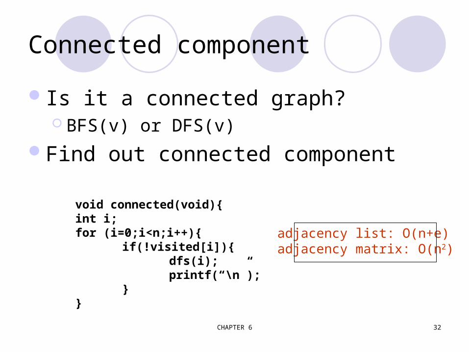
Connected component
Is it a connected graph? BFS(v) or DFS(v)
Find out connected component
void connected(void){int i;for (i=0;i<n;i++){
if(!visited[i]){dfs(i);printf(“\n”);
}}
adjacency list: O(n+e)adjacency matrix: O(n2)

CHAPTER 6 33
Spanning Tree
A spanning tree is a minimal subgraph G’, such that V(G’)=V(G) and G’ is connected
Weight and MST3 1 2
2 3 0
1 3 0
210
0
1 2
3
G1
0
1 2
3
0
1 2
3
DFS(0) BFS(0)

CHAPTER 6 34
Spanning Trees
Either dfs or bfs can be used to create a spanning tree When dfs is used, the resulting spanning tree is
known as a depth first spanning tree When bfs is used, the resulting spanning tree is
known as a breadth first spanning tree
While adding a nontree edge into any spanning tree, this will create a cycle

CHAPTER 6 35
DFS VS BFS Spanning Tree
0
1 2
3 4 5 6
7
0
1 2
3 4 5 6
7
DFS Spanning BFS Spanning
0
1 2
3 4 5 6
7 nontree edgecycle

CHAPTER 6 36
Biconnected components
Definition: Articulation point ( 關節點 ) 原文請參閱課本 如果將 vertex v 以及連接的所有 edge 去除 , 產生 graph
G’, G’ 至少有兩個 connected component, 則 v 稱為 articulation point
Definition: Biconnected graph 定義為無 Articulation point 的 connected graph
Definition: Biconnected component Graph G 中的 Biconnected component H, 為 G 中最大
的 biconnected subgraph; 最大是指 G 中沒有其他 subgraph 是 biconnected 且包含入 H

CHAPTER 6 37
1
3 5
6
0 8 9
7 2
4
connected graph
1
3 5
6
0 8 9
7 2
4
1
3 5
6
0 8 9
7 2
4
two connected components one connected graph
0
1 2
3 4 5 6
7
biconnectedgraph

CHAPTER 6 38
biconnected component: a maximal connected subgraph H(no subgraph that is both biconnected and properly contains H)
1
3 5
6
0 8 9
7 2
4
1
0
1
3
2
4
3 5
8
7
9
7
5
6
7
biconnected components為何沒有任一個邊可能存在於兩個或多個biconnected component 中 ?

CHAPTER 6 39
dfn() and low()
Observation 若 root 有兩個以上 child, 則為 articulation point 若 vertex u 有任一 child w, 使得 w 及 w 後代無法透過 ba
ck edge 到 u 的祖先 , 則為 articulation point
low(u): u 及後代 , 其 back edge 可達 vertex 之最小 dfn() low(u) = min{ dfn(u), min{low(w)|w 是 u 的 child}, min{dfn
(w)|(u,w) 是 back edge}}
u: articulation pointlow(child) dfn(u)

CHAPTER 6 40
Find biconnected component of a connected undirected graphby depth first spanning tree
8 9
1
4 0
3 0 5 3 5
4 61 6
9 8 9 8
7 7
3
4 5
7
6
9 8
2
0
1
0
6
7
1 5
2
4
3
(a) depth first spanning tree (b)
2 2
dfndepthfirst
number
nontreeedge
(back edge)
nontreeedge
(back edge)
Why is cross edge impossible?
If u is an ancestor of v then dfn(u) < dfn(v).

CHAPTER 6 41
*Figure 6.24: dfn and low values for dfs spanning tree with root =3(p.281)
Vertax 0 1 2 3 4 5 6 7 8 9
dfn 4 3 2 0 1 5 6 7 9 8
low 4 0 0 0 0 5 5 5 9 8

CHAPTER 6 42 8 9
3
4 5
7
6
9 8
2
0
1
6
7
1 5
2
4
3
vertex dfn low child low_child low:dfn0 4 4 (4,n,n) null null null:41 3 0 (3,4,0) 0 4 4 3 2 2 0 (2,0,n) 1 0 0 < 23 0 0 (0,0,n) 4,5 0,5 0,5 0 4 1 0 (1,0,n) 2 0 0 < 15 5 5 (5,5,n) 6 5 5 5 6 6 5 (6,5,n) 7 5 5 < 67 7 5 (7,8,5) 8,9 9,8 9,8 7 8 9 9 (9,n,n) null null null, 99 8 8 (8,n,n) null null null, 8

CHAPTER 6 43
*Program 6.5: Initializaiton of dfn and low (p.282)
void init(void) { int i; for (i = 0; i < n; i++) { visited[i] = FALSE; dfn[i] = low[i] = -1; } num = 0; }

CHAPTER 6 44
*Program 6.4: Determining dfn and low (p.282)
Initial call: dfn(x,-1)
low[u]=min{dfn(u), …}
low[u]=min{…, min{low(w)|w is a child of u}, …}
low[u]=min{…,…,min{dfn(w)|(u,w) is a back edge}
dfn[w]0 非第一次,表示藉 back edge
v
u
w
v
u
XO
void dfnlow(int u, int v){/* compute dfn and low while performing a dfs search beginning at vertex u, v is the parent of u (if any) */ node_pointer ptr; int w; dfn[u] = low[u] = num++; for (ptr = graph[u]; ptr; ptr = ptr ->link) { w = ptr ->vertex; if (dfn[w] < 0) { /*w is an unvisited vertex */ dfnlow(w, u); low[u] = MIN2(low[u], low[w]); } else if (w != v) low[u] =MIN2(low[u], dfn[w] ); }}

CHAPTER 6 45
*Program 6.6: Biconnected components of a graph (p.283)
low[u]=min{dfn(u), …}
(1) dfn[w]=-1 第一次(2) dfn[w]!=-1非第一次,藉 back edge
void bicon(int u, int v){/* compute dfn and low, and output the edges of G by their biconnected components , v is the parent ( if any) of the u (if any) in the resulting spanning tree. It is assumed that all entries of dfn[ ] have been initialized to -1, num has been initialized to 0, and the stack has been set to empty */ node_pointer ptr; int w, x, y; dfn[u] = low[u] = num ++; for (ptr = graph[u]; ptr; ptr = ptr->link) { w = ptr ->vertex; if ( v != w && dfn[w] < dfn[u] ) add(&top, u, w); /* add edge to stack */

CHAPTER 6 46
if(dfn[w] < 0) {/* w has not been visited */ bicon(w, u); low[u] = MIN2(low[u], low[w]); if (low[w] >= dfn[u] ){ articulation point printf(“New biconnected component: “); do { /* delete edge from stack */ delete(&top, &x, &y); printf(“ <%d, %d>” , x, y); } while (!(( x = = u) && (y = = w))); printf(“\n”); } } else if (w != v) low[u] = MIN2(low[u], dfn[w]); } }
low[u]=min{…, …, min{dfn(w)|(u,w) is a back edge}}
low[u]=min{…, min{low(w)|w is a child of u}, …}

CHAPTER 6 47
Minimum-cost spanning trees (MST) in a given graph
A minimum-cost spanning tree is a spanning tree of least cost
Design strategy – greedy method Kruskal’s algorithm
Edge by edge Prim’s algorithm
Span out from one vertex Sollin’s algorithm
Hint: Construct from connected components Leave as a homework

CHAPTER 6 48
Greedy Strategy
An optimal solution is constructed in stages At each stage, the best decision is made at this
time Since this decision cannot be changed later,
we make sure that the decision will result in a feasible solution
Typically, the selection of an item at each stage is based on a least cost or a highest profit criterion

CHAPTER 6 49
Kruskal’s Idea
Build a minimum cost spanning tree T by adding edges to T one at a time
Select the edges for inclusion in T in nondecreasing order of the cost
An edge is added to T if it does not form a cycle
Since G is connected and has n > 0 vertices, exactly n-1 edges will be selected

CHAPTER 6 50
Examples for Kruskal’s Algorithm
0
1
2
34
5 6
0
1
2
34
5 6
28
16
121824
22
25
1014
0
1
2
34
5 6
10
0 5
2 3
1 6
1 2
3 6
3 4
4 6
4 5
0 1
10
12
14
16
18
22
24
25
28 6/9

CHAPTER 6 51
0
1
2
34
5 6
10
12
0
1
2
34
5 6
10
12
14
0
1
2
34
5 6
10
12
14 16
0 5
2 3
1 6
1 2
3 6
3 4
4 6
4 5
0 1
10
12
14
16
18
22
24
25
28 + 3 6
cycle

CHAPTER 6 52
0 5
2 3
1 6
1 2
3 6
3 4
4 6
4 5
0 1
10
12
14
16
18
22
24
25
28
0
1
2
34
5 6
10
12
14 16
22
0
1
2
34
5 6
10
12
14 16
22
25
4 6
cycle
+
cost = 10 +25+22+12+16+14

CHAPTER 6 53
Kruskal’s algorithmEdge by edgeO(e log e)Algorithm:
T={};While ((T contains less than n-1 edges) &&(E not empty)){
choose an edge (v,w) from E of lowest cost;delete (v,w) from E;if((v,w) does not create a cycle in T)
add(v,w) to T;else
discard(v,w);}If(T contains fewer than n – 1 edges)
printf(“No spanning tree\n”);

CHAPTER 6 54
Prim’s algorithmBegins from a vertexO(n2)Algorithm:
T={};TV = {0}; /* start with vertex 0 and no edges */While (T contains fewer than n-1 edges){
let(u,v) be a least cost edge s.t. u in TV and v not in TV;if (there is no such edge)
break;add v to TV;add (u,v) to T;
}If (T contains fewer than n-1 edges)
printf(“No spanning tree\n”);

CHAPTER 6 55
Examples for Prim’s Algorithm
0
1
2
34
5 6
0
1
2
34
5 6
10
0
1
2
34
5 6
1010
25 25
22
0
1
2
34
5 6
28
16
121824
22
25
1014

CHAPTER 6 56
0
1
2
34
5 6
10
25
22
12
0
1
2
34
5 6
10
25
22
12
16
0
1
2
34
5 6
10
25
22
12
1614
0
1
2
34
5 6
28
16
121824
22
25
1014

CHAPTER 6 57
Sollin’s Algorithm
0
1
2
34
5 6
10
0
22
12
1614
0
1
2
34
5 6
10
22
12
14
0
1
2
34
5 6
0
1
2
34
5 6
28
16
121824
22
25
1014
vertex edge0 0 -- 10 --> 5, 0 -- 28 --> 11 1 -- 14 --> 6, 1-- 16 --> 2, 1 -- 28 --> 02 2 -- 12 --> 3, 2 -- 16 --> 13 3 -- 12 --> 2, 3 -- 18 --> 6, 3 -- 22 --> 44 4 -- 22 --> 3, 4 -- 24 --> 6, 5 -- 25 --> 55 5 -- 10 --> 0, 5 -- 25 --> 46 6 -- 14 --> 1, 6 -- 18 --> 3, 6 -- 24 --> 4
{0,5}
5 4 0 125 28
{1,6}
1 216 281
6 3 6 418 24
CHAPTER 6 58
Is there a path? How short it can be?
Single source/ All destinations Nonnegative edge costs General weights
All-pairs shortest pathTransitive closure

CHAPTER 6 59
Single source all destinationsDijkstra’s algorithm
A spanning tree againFor nonnegative edge costs (Why?)Start from a vertex v, greedy methoddist[w]: the shortest length to w through S
v
u
w
length(<u,w>)
dist[w]
dist[u]

CHAPTER 6 60
*Figure 6.29: Graph and shortest paths from v0 (p.293)
V0 V4V1
V5V3V2
50 10
20 10 15 20 35 30
15 3
45
(a)
path length1) v0 v2 102) v0 v2 v3 253) v0 v2 v3 v1 454) v0 v4 45
(b)
Single Source All Destinations
Determine the shortest paths from v0 to all the remaining vertices.

CHAPTER 6 61
Example for the Shortest Path
0
1 23
4
5
67
SanFrancisco Denver
Chicago
Boston
NewYork
Miami
New Orleans
Los Angeles
300 1000
8001200
1500
1400
1000
9001700
1000250
0 1 2 3 4 5 6 70 01 300 02 1000 800 03 1200 04 1500 0 2505 1000 0 900 14006 0 10007 1700 0
Cost adjacency matrix

CHAPTER 6 62
43
5
1500
250
43
5
1500
250
1000
選 5 4到 3由 1500改成 1250
4
5
250
6900
4到 6由改成 1250
4
5
250
7 1400
4到 7由改成 1650
4
5
250
6900
7 1400
3
1000
選 6
4
5
250
6900
7 1400
1000
4-5-6-7比 4-5-7長
(a) (b) (c)
(d) (e) (f)

CHAPTER 6 63
4
5
250
6900
7 1400
3
1000
選 3
4
5
250
6900
7 1400
3
1000
2 1200
4到 2由改成 2450
4
5
250
6900
7 1400
3
1000
2 1200
選 7
4
5
250
7 1400
0
4到 0由改成 3350
(g) (h)
(i)(j)

CHAPTER 6 64
Example for the Shortest Path(Continued)
Iteration S VertexSelected
LA[0]
SF[1]
DEN[2]
CHI[3]
BO[4]
NY[5]
MIA[6]
NO
Initial -- ---- + + + 1500 0 250 + +
1 {4} 5 + + + 1250 0 250 1150 16502 {4,5} 6 + + + 1250 0 250 1150 16503 {4,5,6} 3 + + 2450 1250 0 250 1150 16504 {4,5,6,3} 7 3350 + 2450 1250 0 250 1150 16505 {4,5,6,3,7} 2 3350 3250 2450 1250 0 250 1150 16506 {4,5,6,3,7,2} 1 3350 3250 2450 1250 0 250 1150 16507 {4,5,6,3,7,2,1}
(a)(b) (c) (d)
(e)(f)
(g)(h)
(i)(j)

CHAPTER 6 65
Data Structure for SSAD
#define MAX_VERTICES 6int cost[][MAX_VERTICES]= {{ 0, 50, 10, 1000, 45, 1000}, {1000, 0, 15, 1000, 10, 1000}, { 20, 1000, 0, 15, 1000, 1000}, {1000, 20, 1000, 0, 35, 1000}, {1000, 1000, 30, 1000, 0, 1000}, {1000, 1000, 1000, 3, 1000, 0}};int distance[MAX_VERTICES];short int found{MAX_VERTICES];int n = MAX_VERTICES;
adjacency matrix

CHAPTER 6 66
shortest()
Void shortestpath(int v, int cost[][MAX_VERTICES], int dist [], int n, int found[]){
int i,u,w;for (i=0;i<n;i++) {
found[i]=FALSE;dist [i] = cost[v][i];
}found[v]=TRUE;dist [v]=0;for(i=0;i<n-2;i++){
u=choose(dist,n,found);found[u]=TRUE;for(w=0;w<n;w++)
if(dist [u]+cost[u][w] < dist [w])dist [w] = dist [u]+cost[u][w];
}} O(n2)

CHAPTER 6 67
Single source all destinationsBellmanFord algorithm
For general weightsPath has at most n-1 edges, otherwise…distk[u]: from v to u, has at most k edges ]}}][[][{min],[min{][ 11 uilengthidistudistudist k
i
kk
0
1
2
3
4
5
6
6
5
5
1
-1
-2
-2
-1
3
33405310
5405310
7425310
455330
5560
6543210

CHAPTER 6 68
BellmanFord()
Void BellmanFord(int n, int v) {
int i,k;for (i =0;i<n;i++)
dist[i] = length[v][i];for(k=2;k<=n-1;k++)
for(each u s.t. u!=v and u has at least one incoming edge)for(each <i,u> in the graph)
if(dist([u]>dist[i]+length[i][u])dist[u]=dist[i]+length[i][u];
}
O(n^3)

CHAPTER 6 69
All-Pairs shortest paths
執行 n 次 single source all destinations algo.Dynamic programming strategy
利用 recursive formula 來表示 好好地 implement recursive formula, 用 table 輔助
Ak[i][j] ≡ shortest length from i to j through no intermediate vertex greater than k
A-1[i][j] = length[i][j]Ak[i][j] = min{Ak-1[i][j], Ak-1[i][k]+ Ak-1[k][j], k≥0

CHAPTER 6 70
AllLengths()
Void AllLength(int n){
int i,j,k;for(i=0;i<n;i++)
for(j=0;j<n;j++)a[i][j] = length[i][j];
for(k=0;k<n;k++)for(i=0;i<n;i++)
for(j=0;j<n;j++)if((a[i][k]+a[k][j])<a[i][j])
a[i][j] = a[i][k]+a[k][j];}
O(n^3)
0 1
2
6
4
211
3

CHAPTER 6 71
Transitive closure
Definition: transitive closure matrix, A+
A+[i][j] = 1, if there’s a path of length > 0 from i to j A+[i][j] = 0, otherwise
Definition: reflexive transitive closure matrix, A* A*[i][j] = 1, if there’s a path of length >= 0 from i to j A*[i][j] = 0, otherwise
O(n^3), by AllLengths() O(n^2), an undirected graph, by connected chec
k

CHAPTER 6 72
Activity on Vertex (AOV) Network definitionA directed graph in which the vertices represent tasks or activities and the edges represent precedence relations between tasks.predecessor (successor)vertex i is a predecessor of vertex j iff there is a directed path from i to j. j is a successor of i.partial ordera precedence relation which is both transitive (i, j, k, ij & jk => ik ) and irreflexive (x xx).acyclic grapha directed graph with no directed cycles

CHAPTER 6 73
*Figure 6.38: An AOV network (p.305)
Topological order:linear ordering of verticesof a graphi, j if i is a predecessor ofj, then i precedes j in thelinear ordering
C1, C2, C4, C5, C3, C6, C8,C7, C10, C13, C12, C14, C15, C11, C9
C4, C5, C2, C1, C6, C3, C8,C15, C7, C9, C10, C11, C13,C12, C14

CHAPTER 6 74
*Program 6.13: Topological sort (p.306)
for (i = 0; i <n; i++) { if every vertex has a predecessor { fprintf(stderr, “Network has a cycle. \n “ ); exit(1); } pick a vertex v that has no predecessors; output v; delete v and all edges leading out of v from the network;}

CHAPTER 6 75
*Figure 6.39:Simulation of Program 6.13 on an AOV network (p.306)
v0 no predecessordelete v0->v1, v0->v2, v0->v3 v1, v2, v3 no predecessor
select v3delete v3->v4, v3->v5
select v2delete v2->v4, v2->v5
select v5
select v1delete v1->v4

CHAPTER 6 76
Issues in Data Structure Consideration
Decide whether a vertex has any predecessors.–Each vertex has a count.
Decide a vertex together with all its incident edges.
–Adjacency list

CHAPTER 6 77
*Figure 6.40:Adjacency list representation of Figure 6.30(a)(p.309)
0 1 2 3 NULL
1 4 NULL
1 4 5 NULL
1 5 4 NULL
3 NULL
2 NULL
V0
V1
V2
V3
V4
V5
v0
v1
v2
v3
v4
v5
count linkheadnodes
vertex linknode

CHAPTER 6 78
*(p.307)
typedef struct node *node_pointer;typedef struct node { int vertex; node_pointer link; };typedef struct { int count; node_pointer link; } hdnodes;hdnodes graph[MAX_VERTICES];

CHAPTER 6 79
*Program 6.14: Topological sort (p.308)
O(n)
void topsort (hdnodes graph [] , int n){ int i, j, k, top; node_pointer ptr; /* create a stack of vertices with no predecessors */ top = -1; for (i = 0; i < n; i++) if (!graph[i].count) {no predecessors, stack is linked through graph[i].count = top; count field top = i; }for (i = 0; i < n; i++) if (top == -1) { fprintf(stderr, “\n Network has a cycle. Sort terminated. \n”); exit(1);}

CHAPTER 6 80
O(e)
O(e+n)
Continued} else { j = top; /* unstack a vertex */ top = graph[top].count; printf(“v%d, “, j); for (ptr = graph [j]. link; ptr ;ptr = ptr ->link ){ /* decrease the count of the successor vertices of j */ k = ptr ->vertex; graph[k].count --; if (!graph[k].count) { /* add vertex k to the stack*/ graph[k].count = top; top = k; } } } }

CHAPTER 6 81
Activity on Edge (AOE) Networks
directed edge–tasks or activities to be performed
vertex–events which signal the completion of certain activities
number–time required to perform the activity

CHAPTER 6 82
*Figure 6.41:An AOE network(p.310)
concurrent

CHAPTER 6 83
Application of AOE Network
Evaluate performance–minimum amount of time
–activity whose duration time should be shortened
–…
Critical path–a path that has the longest length
–minimum time required to complete the project
–v0, v1, v4, v7, v8 or v0, v1, v4, v6, v8 (18)

CHAPTER 6 84
other factorsEarliest time that vi can occur
–the length of the longest path from v0 to vi
–the earliest start time for all activities leaving vi
–early(6) = early(7) = 7Latest time of activity
–the latest time the activity may start without increasing the project duration
–late(5)=8, late(7)=7
Critical activity–an activity for which early(i)=late(i)
–early(7)=late(7)
late(i)-early(i)–measure of how critical an activity is
–late(5)-early(5)=8-5=3

CHAPTER 6 85
v0
v1
v2
v3
v4
v5
v6
v7
v8
a0=6
a1=4
a2=5
a3=1
a4=1
a5=2
a6=9
a7=7
a9=2
a10=4
a8=4
earliest, early, latest, late
0
0
6
6
77
16
16
18
0
44 7
1414
0
55
7
7
0
06
6
7
7
16
10
18
2
6
6
14
14
14
108
8
3
CHAPTER 6 86
Determine Critical Paths
Delete all noncritical activitiesGenerate all the paths from the start to finish vertex.
CHAPTER 6 87
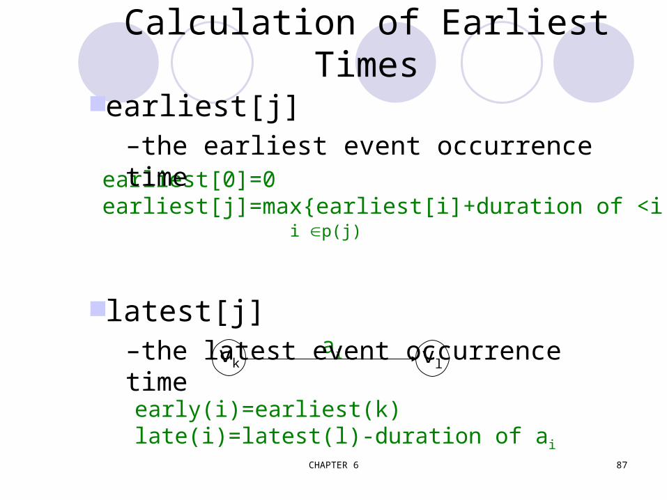
Calculation of Earliest Times
vk vlai
early(i)=earliest(k)late(i)=latest(l)-duration of ai
earliest[0]=0earliest[j]=max{earliest[i]+duration of <i,j>}
i p(j)
earliest[j]–the earliest event occurrence time
latest[j]–the latest event occurrence time
CHAPTER 6 88
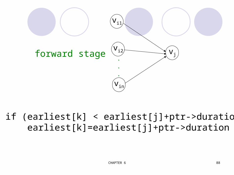
vi1
vi2
vin
.
.
.
vjforward stage
if (earliest[k] < earliest[j]+ptr->duration) earliest[k]=earliest[j]+ptr->duration

CHAPTER 6 89
*Figure 6.42:Computing earliest from topological sort (p.313)
v0
v1
v2
v3
v4
v6
v7
v8
v5

CHAPTER 6 90
Calculation of Latest Timeslatest[j]
the latest event occurrence time
latest[n-1]=earliest[n-1]latest[j]=min{latest[i]-duration of <j,i>}
i s(j) vi1
vi2
vin
.
.
.
vj backward stage
if (latest[k] > latest[j]-ptr->duration) latest[k]=latest[j]-ptr->duration

CHAPTER 6 91
*Figure 6.43: Computing latest for AOE network of Figure 6.41(a)(p.314)

CHAPTER 6 92
*Figure 6.43(continued):Computing latest of AOE network of Figure 6.41(a)(p.315)
latest[8]=earliest[8]=18 latest[6]=min{earliest[8] - 2}=16 latest[7]=min{earliest[8] - 4}=14 latest[4]=min{earliest[6] - 9;earliest[7] -7}= 7 latest[1]=min{earliest[4] - 1}=6 latest[2]=min{earliest[4] - 1}=6 latest[5]=min{earliest[7] - 4}=10 latest[3]=min{earliest[5] - 2}=8 latest[0]=min{earliest[1] - 6;earliest[2]- 4; earliest[3] -5}=0(c)Computation of latest from Equation (6.4) using a reverse topological order

CHAPTER 6 93
*Figure 6.44:Early, late and critical values(p.316)
Activity Early Late Late-Early
Critical
a0
a1
a2
a3
a4
a5
a6
a7
a8
a9
a10
0006457771614
02366877101614
02302300300
YesNoNoYesNoNoYesYesNoYesYes

CHAPTER 6 94
*Figure 6.45:Graph with noncritical activities deleted (p.316)
V0V4
V8
V1V6
V7
a0a3 a6
a7a10
a9

CHAPTER 6 95
*Figure 6.46: AOE network with unreachable activities (p.317)
V0
V3
V1
V5
V2
V4
a0
a1
a2
a3
a5 a6
a4
earliest[i]=0

CHAPTER 6 96
*Figure 6.47: an AOE network(p.317)
V5 V8 V9
a10=5 a13=2
V2 V4 V7a4=3 a9=4
V1 V3 V6
a2=3 a6=4
V0
a12=4
a11=2a8=1
a7=4
a5=3a3=6
a0=5
a1=6
start finish