chapter 6 supply and demand dynamicss3-euw1-ap-pe-ws4-cws-documents.ri-prod.s3.amazonaws.com/... ·...

Chapter 6Supply and demand dynamics

O. Afonso, P. B. Vasconcelos

Computational Economics: a concise introduction

O. Afonso, P. B. Vasconcelos Computational Economics 1 / 26

Overview

1 Introduction

2 Economic model

3 Numerical solution

4 Computational implementation

5 Numerical results and simulation

6 Highlights

7 Main references


Introduction

In 1930, Ricci, Tinbergen and Shultz published studies containing the firstexplicit cobweb model(s).

It is considered that the quantity supplied is a function of the price of thepreceding time period.Then, by describing cyclical supply and demand, it explains why pricescan be subject to periodic fluctuations.For some slopes of the demand and supply curves, the equilibrium canbe reached.

The assumption that supply must equal demand can be relaxed, as in thecase of the market model with inventory.

Since supply reacts with a one–period lag to market prices, producershave an inventory to meet unexpected demand.

These models are presented to illustrate the use of first-order differenceequations in economic analysis, following Gandolfo (2010), Chiang (2005)and Pashigian (2008).


Economic model

Cobweb model

The cobweb model is based on a time lag between supply and demanddecisions.

Producer’s output decision must be made one period in advance;suppose that producers go to market with an unusually small production.This shortage results in high prices and if producers expect these highprice conditions to continue in the following period, they will raise theproduction and, as a result, prices decrease.If low prices are expected to continue, producers will decrease theproduction, resulting again in higher prices.Thus, oscillating between periods of low supply with high prices and highsupply with low prices, the set price-quantity traces out a spiral.This set may spiral inwards and the economy converges to theequilibrium or it may spiral outwards and the economy diverges since thefluctuations increase in magnitude:

there is convergence if the supply curve is steeper than the demand curve,and vice versa.


Economic model

Assume that the output decisions in time t are based on the current price, Pt ;thus, Pt determines Qs,t+1 or, equivalently, Pt−1 affects Qs,t , which, interactingwith a demand function, imposes dynamic price patterns.The standard equations that characterise the market are:

demand, Qd,t = Qd − aPt ;

supply, Qs,t = Qs + bPt−1;equilibrium, Qd,t = Qs,t .

It is assumed that the price at t is set at a level which clears the market.The endogenous variables are: quantity demanded, Qd,t ; quantityoffered, Qs,t ; and price of the good, Pt .The exogenous variables are: independent/autonomous quantitydemanded, Qd ; and independent/autonomous quantity offered, Qs.Parameters are: a,b > 0, respectively, the sensitivity of the demand toprice at time t and the sensitivity of the supply to price at time t − 1.


Economic model

Demand

Qd,t is the total amount of a good that buyers would choose to purchase giventhe price of the good, Pt , as well as other variables, represented by theexogenous variable Qd .

The Law of Demand states that, ceteris paribus, when the price of a goodrises, the quantity of the good demanded falls.A Demand Curve (or line) is a graphical representation of the relationshipbetween price and quantity demanded, assuming that everything elseremains constant.Changes in demand occur when one of the determinants of demandother than price changes; i.e. ‘when the ceteris are not paribus’.


Economic model

Supply

Qs,t is the total amount of a good that sellers would choose to produce andsell given the price of the good at the previous time period, Pt−1, as well asother variables, represented by the exogenous variable Qs.

The Law of Supply states that, ceteris paribus, when the price of a goodat the previous time period rises, the quantity of the good supplied alsorises.A Supply Curve (or line) is a graphical representation of the relationshipbetween the price in the previous period and quantity supplied (ceterisparibus).Changes in supply occur when one of the determinants of supply otherthan the price of the previous period changes.


Economic model

Putting the demand and the supply curves together

By substituting Qd,t and Qs,t in Qd,t = Qs,t , the model can be reduced to asingle first-order difference equation:

aPt + bPt−1 = Qd −Qs,

which, since a 6= 0, can be rewritten as

Pt+1 = −ba

Pt +Qd −Qs

a. (1)

Now, equation (1) can be rewritten in terms of P0, by replacing Pt by− b

a Pt−1 +Qd−Qs

a and then Pt−1 by − ba Pt−2 +

Qd−Qsa and so on.

Rewriting for t instead of t + 1,

Pt =

(P0 −

Qd −Qs

a + b

)(−b

a

)t

+Qd −Qs

a + b.


Economic model

Three points are crucial in regard to the time path.1 The expression Qd−Qs

a+b can be interpreted as the inter-temporalequilibrium price, which, being constant, is the stationary equilibrium.

2 The sign of P0 − Qd−Qsa+b bears on the question of whether the time path

starts above or below the equilibrium (mirror effect), whereas itsmagnitude decides how far above or below (scale effect).

3 The expression − ba generates an oscillatory time path and, consequently,

gives rise to the cobweb phenomenon, showing three possible varietiesof oscillation patterns:

explosive if b>a;uniform if b=a;damped if b<a.

Indeed it is easy to understand that Pt will converge to Qd−Qsa+b as t tends

to∞ if | − ba | < 1.


Economic model

Market model with inventory

The market model with inventory permits that sellers do keep an inventory ofthe good, assuming that the quantity demanded, Qd,t , and the quantitycurrently produced, Qs,t , are unlagged (linear) functions of Pt .

Sellers, at the beginning of each period, set a price for that periodbearing in mind the inventory situation.

The model is summarised by:demand, Qd,t = Qd − aPt ;

supply, Qs,t = Qs + bPt ;price-setting, Pt+1 = Pt − σ (Qs,t −Qd,t);

where σ > 0 is the (inventory) price-adjustment parameter.


Economic model

Market model with inventory

By substituting the demand and supply equations in the price-setting equation,the model can be condensed into a single first-order difference equation,

Pt+1 = (1− σ (a + b))Pt + σ(

Qd −Qs

), (2)

and the solution is given by

Pt =

(P0 −

Qd −Qs

a + b

)(1− σ (a + b))t +

Qd −Qs

a + b.

The dynamic stability of the model will hinge on the expression 1− σ (a + b).The method converges whenever |1− σ (a + b)| < 1, that is, for 0 < σ < 2

a+b .


Numerical solution

Difference equations

Dynamical systems describe the evolution of certain quantities over time, andhere time is considered to be discrete.

A first–order discrete dynamic system is a sequence of numbers given bya relation (first–order difference equation) yt+1 = f (yt), where f (yt) canbe linear or not, giving rise to linear and nonlinear difference equations.If the system depends also on t itself, then it is said to benonautonomous and autonomous otherwise.Equations (1) and (2) are of the form yt+1 = f (yt) + g(t), with g(t) aconstant function, both examples of autonomous first order differenceequations; they are also nonhomogeneous since g(t) 6= 0, otherwise theywould be homogeneous.


Numerical solution

Difference equationsAn nth–order difference equation involves more than one–period time lag,yt+n = f (yt+n−1, ..., yt).

The solution of a nonhomogeneous linear equation

yt+n +∑

i=1,...,n

cn−iyt+n−i = g(t)

with constant coefficients cn−1, ..., c0, can be obtained from the sum ofa complementary function, yc , solution of the homogeneous part, and witha particular solution, yp, any solution of the nonhomogeneous part.

For a first–order problem, a complementary solution can be obtained bytrying a solution of the form kλt , giving rise to

yt = kλt + yp,

where k is specified provided that an initial condition at t = 0 is given.The particular solution can be interpreted as the equilibrium state andyt − yp = kλt gives the deviation from the equilibrium.


Numerical solution


The stability of the solution depends on the complementarity solution;when t →∞ the solution is convergent (divergent) if |λ| < 1 (|λ| > 1);furthermore, the cases |λ| = 1 are also divergent;if λ < 0 (λ > 0) the time path of λt is oscillatory (nonoscillatory).

For the cobweb model, λ = − ba and since both a and b are positive, oscillatory

behaviour is shown.


Numerical solution


For a second–order problem, the solution of the complementarity problem isobtained trying a solution of the form λt in yt+2 + c1yt+1 + c0yt = 0:

λt+2 + c1λt+1 + c0λ

t = 0

λ2 + c1λ+ c0 = 0 (3)

for λ 6= 0. The two sought roots of the second–order (characteristic)polynomial are the solution of equation (3), the characteristic equation:

if λ1, i = 1,2 are distinct real roots, yt = k1λt1 + k2λ

t2, for two constants k1

and k2;if λ = λ1 = λ2, yt = k1λ

t + k2tλt , for two constants k1 and k2;if λ1 = a− ib and λ2 = a + ib are complex (conjugate),yt = ρt(k1cos(wt) + k2sin(wt)), with ρ =

√a2 + b2 and w = tg−1(b/a).


Numerical solution


With respect to stability, convergence will occur:for real distinct roots whenever |λ1| < 1 and |λ2| < 1;for a real root of multiplicity 2 whenever |λ| < 1;for conjugate complex roots when ρ < 1 (with a trigonometric oscillation).

For an nth–order difference linear equation, solutions are combinations ofthose presented for the second–order and the path towards the equilibrium isgoverned by the n roots of an nth–order polynomial.Linear difference equations, with constant coefficients, play an important rolein scientific problems, particularly in economics:

the convergence behaviour of the time path can be well understood.Nonlinear equations are far more difficult to solve (analytically) than the linearcounterpart since many of them are not solvable in terms of elementaryfunctions; nevertheless, solutions can be obtained by iterating the equationnumerically on a computer easily.


Numerical solution

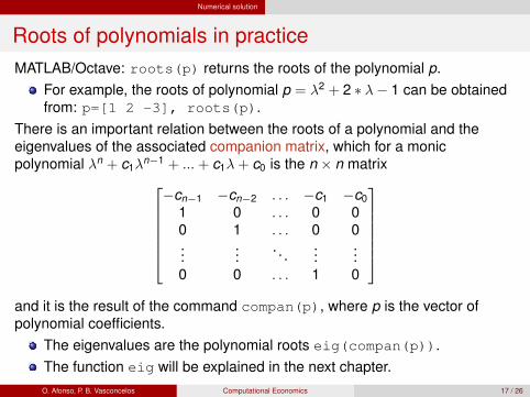
Roots of polynomials in practiceMATLAB/Octave: roots(p) returns the roots of the polynomial p.

For example, the roots of polynomial p = λ2 + 2 ∗ λ− 1 can be obtainedfrom: p=[1 2 -3], roots(p).

There is an important relation between the roots of a polynomial and theeigenvalues of the associated companion matrix, which for a monicpolynomial λn + c1λ

n−1 + ...+ c1λ+ c0 is the n × n matrix−cn−1 −cn−2 . . . −c1 −c0

1 0 . . . 0 00 1 . . . 0 0...

.... . .

......

0 0 . . . 1 0

and it is the result of the command compan(p), where p is the vector ofpolynomial coefficients.

The eigenvalues are the polynomial roots eig(compan(p)).The function eig will be explained in the next chapter.O. Afonso, P. B. Vasconcelos Computational Economics 17 / 26

Computational implementation

The following baseline values are considered:Qd = 1000, Qs = 250, a = 10 and b = 5.



Presentation and parameters

%% Cobweb model% Implemented by : P .B . Vasconcelos and O. Afonsoclear ; clc ;disp ( ’−−−−−−−−−−−−−−−−−−−−−−−−−−−−−−−−−−−−−−−−−−−−−−−−−−−−−−−−− ’ ) ;disp ( ’Cobweb model ’ ) ;disp ( ’−−−−−−−−−−−−−−−−−−−−−−−−−−−−−−−−−−−−−−−−−−−−−−−−−−−−−−−−− ’ ) ;

%% parametersa = 10; % s e n s i t i v i t y o f the demand to p r i ceb = 5; % s e n s i t i v i t y o f the supply to p r i ce

%% exogenous v a r i a b l e sQd_bar = 1000; % independent / autonomous q u a n t i t y demandedQs_bar = 250; % independent / autonomous q u a n t i t y o f f e red

%% modelf p r i n t f ( ’Qd, t = %g − %g∗Pt \ n ’ , Qd_bar , a ) % demandf p r i n t f ( ’Qs , t = %g + %g∗Pt−1 \ n ’ , Qs_bar , b ) % supplyf p r i n t f ( ’Qd, t = Qs, t \ n ’ )



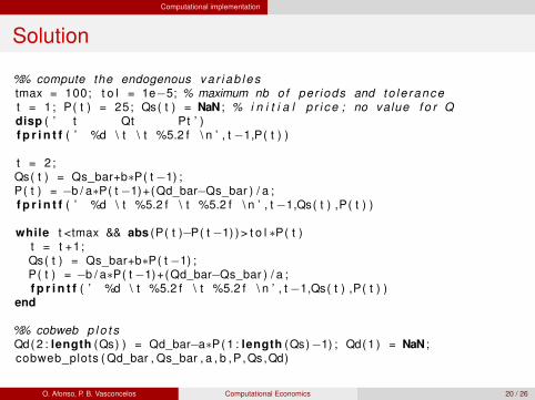
Solution

%% compute the endogenous va r i a b l e stmax = 100; t o l = 1e−5; % maximum nb of per iods and to le rancet = 1 ; P( t ) = 25; Qs( t ) = NaN ; % i n i t i a l p r i ce ; no value f o r Qdisp ( ’ t Qt Pt ’ )f p r i n t f ( ’ %d \ t \ t %5.2 f \ n ’ , t −1,P( t ) )

t = 2 ;Qs( t ) = Qs_bar+b∗P( t −1) ;P( t ) = −b / a∗P( t −1)+(Qd_bar−Qs_bar ) / a ;f p r i n t f ( ’ %d \ t %5.2 f \ t %5.2 f \ n ’ , t −1,Qs( t ) ,P( t ) )

while t <tmax && abs (P( t )−P( t −1) ) > t o l ∗P( t )t = t +1;Qs( t ) = Qs_bar+b∗P( t −1) ;P( t ) = −b / a∗P( t −1)+(Qd_bar−Qs_bar ) / a ;f p r i n t f ( ’ %d \ t %5.2 f \ t %5.2 f \ n ’ , t −1,Qs( t ) ,P( t ) )

end

%% cobweb p l o t sQd( 2 : length (Qs) ) = Qd_bar−a∗P( 1 : length (Qs)−1) ; Qd( 1 ) = NaN ;cobweb_plots ( Qd_bar , Qs_bar , a , b ,P, Qs,Qd)



Cobweb plots

function cobweb_plots ( Qd_bar , Qs_bar , a , b ,P, Qs,Qd)% Cobweb p l o t s : p r ice , q u a n t i t y cobweb p lo t , p r i ce phase diagram

% p l o t ax is l i m i t symin = min (P) ∗ . 95 ; ymax = max(P) ∗1.05 ;yy = [ ymin , ymax ] ;

% pr i cessubplot (2 ,2 ,1 )t = 0 : length (Qs)−1;plot ( t ,P) ; xlabel ( ’ t ’ ) ; ylabel ( ’P ’ ) ; y l im ( yy ) ;

% cobweb p l o tsubplot (2 ,2 ,2 )Pt = l inspace ( ymin , ymax , length (P) ) ’ ;plot ( [ Qd_bar−a∗Pt Qs_bar+b∗Pt ] , Pt , ’−− ’ ) ;xlabel ( ’Q ’ ) ; ylabel ( ’P ’ ) ; y l im ( yy ) ;hold on ;for t = 1 : length (P)−1

plot ( [ Qs_bar+b∗P( t ) , Qd_bar−a∗P( t ) ] , [ P( t ) ,P( t ) ] , ’ r ’ ) ;plot ( [ Qd_bar−a∗P( t ) , Qs_bar+b∗P( t +1) ] , [ P( t ) ,P( t +1) ] , ’ r ’ ) ;

endhold o f f



Cobweb plots

% phase diagram ( p r i ce )subplot (2 ,2 ,3 )plot ( [ 0 , ymax ] , [ 0 , ymax ] ) ;yy = [P( 1 ) ∗0.95 ,ymax ] ;hold on ;for t = 1 : length (P)−1

plot ( [ P( t ) ,P( t ) ] , [ P( t ) ,P( t +1) ] , ’ r ’ ) ;plot ( [ P( t ) ,P( t +1) ] , [ P( t +1) ,P( t +1) ] , ’ r ’ ) ;

endxlabel ( ’P_{ t } ’ ) ; ylabel ( ’P_{ t +1} ’ ) ;x l im ( yy ) ; y l im ( yy ) ;hold o f f

% q u a n t i t i e s demanded and supp l iedsubplot (2 ,2 ,4 )t = 0 : length (Qs)−1;plot (Qs , t , ’− ’ ,Qd, t , ’−− ’ ) ;xlabel ( ’Q ’ ) ; ylabel ( ’ t ’ ) ; legend ( ’Q_s ’ , ’Q_d ’ ) ;

end


Numerical results and simulation

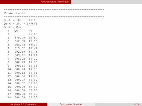
---------------------------------------------------------Cobweb model---------------------------------------------------------Qd,t = 1000 - 10*PtQs,t = 250 + 5*Pt-1Qd,t = Qs,tt Qt Pt0 25.001 375.00 62.502 562.50 43.753 468.75 53.124 515.62 48.445 492.19 50.786 503.91 49.617 498.05 50.208 500.98 49.909 499.51 50.0510 500.24 49.9811 499.88 50.0112 500.06 49.9913 499.97 50.0014 500.02 50.0015 499.99 50.0016 500.00 50.0017 500.00 50.0018 500.00 50.00


Numerical results and simulation

0 2 4 6 8 10 12 14 16 18

25

30

35

40

45

50

55

60

65

t

P

(a) price dynamics

400 450 500 550 600 650 700 750

25

30

35

40

45

50

55

60

65

Q

P

(b) Cobweb plot

25 30 35 40 45 50 55 60 65

25

30

35

40

45

50

55

60

65

Pt

Pt+

1

(c) price phase diagram

400 450 500 550 600 650 700 7500

2

4

6

8

10

12

14

16

18

Q

t

Qs

Qd

(d) quantity dynamics

Cobweb plots


Highlights

The cobweb is a dynamic model derived from the static supply–demandmodel.It assumes that supply reacts to price with a lag of one period of time,while demand depends on current price.It explains why prices might be subject to periodic fluctuations in certaintypes of markets.The market model with inventory relaxes the assumption that supply mustequal demand.Difference equations are introduced and specifications aboutconvergence are exposed.


Main references

A. C. Chiang, K. WainwrightFundamental methods of mathematical economics.McGraw-Hill, New York, 2005.

G. GandolfoEconomic dynamics.Springer, 2010.

B. P. PashigianCobweb theorem.In Lawrence Blume and Steven Durlauf, editors, The new Palgravedictionary of economics. Palgram Macmillan, 2008.


chapter 6 supply and demand dynamicss3-euw1-ap-pe-ws4-cws-documents.ri-prod.s3.amazonaws.com/... ·...

Documents