CHAPTER 6CHAPTER 6 Risk Aversion Risk Aversion and Capital and Capital Allocation to Allocation to Risky AssetsRisky Assets

6-2

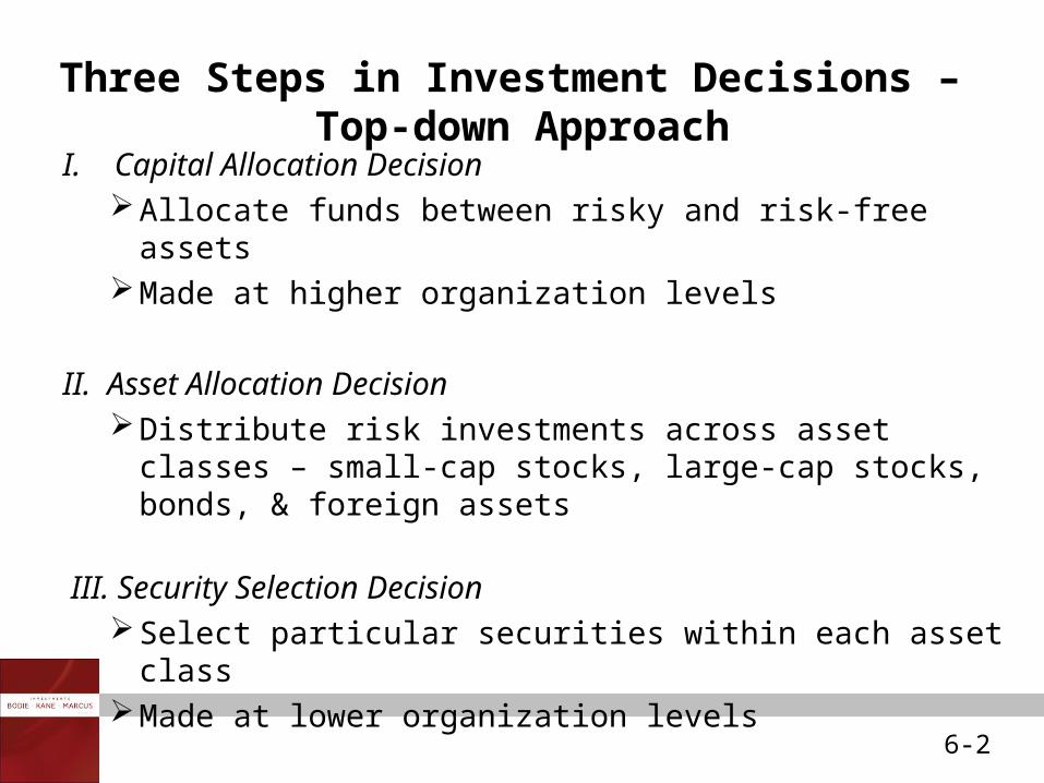
Three Steps in Investment Decisions – Top-down Approach

I. Capital Allocation DecisionAllocate funds between risky and risk-free assetsMade at higher organization levels 

II. Asset Allocation DecisionDistribute risk investments across asset classes – small-

cap stocks, large-cap stocks, bonds, & foreign assets

 III. Security Selection DecisionSelect particular securities within each asset classMade at lower organization levels

6-3

Risk and Risk Aversion

• Speculation– Considerable risk

• Sufficient to affect the decision

– Commensurate gain

• Gamble – Bet or wager on an uncertain outcome

6-4

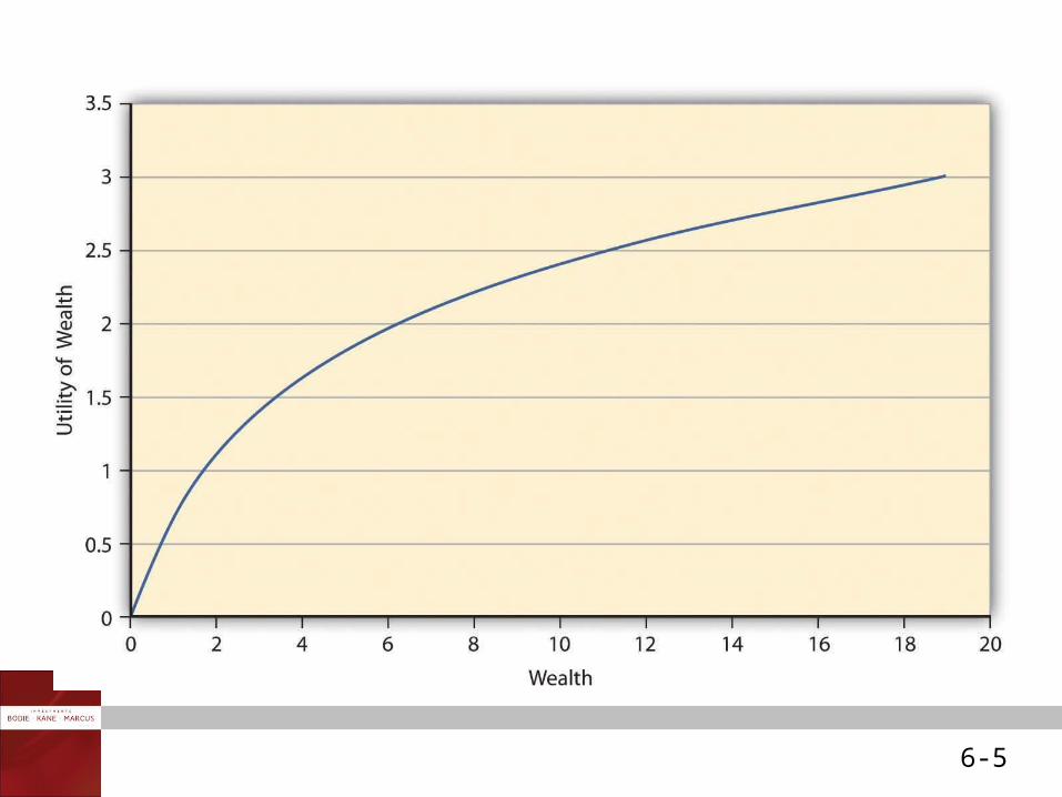
Risk Aversion and Utility Values

• Risk averse investors reject investment portfolios that are fair games or worse

• These investors are willing to consider only risk-free or speculative prospects with positive risk premiums

• Intuitively one would rank those portfolios as more attractive with higher expected returns

6-5

6-6

Table 6.1 Available Risky Portfolios (Risk-free Rate = 5%)

6-7

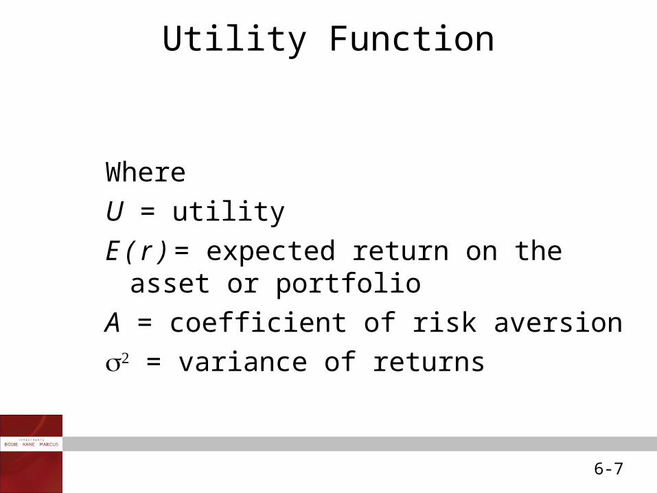
Utility Function

Where

U = utility

E ( r ) = expected return on the asset or portfolio

A = coefficient of risk aversion

= variance of returns

21( )

2U E r A

6-8

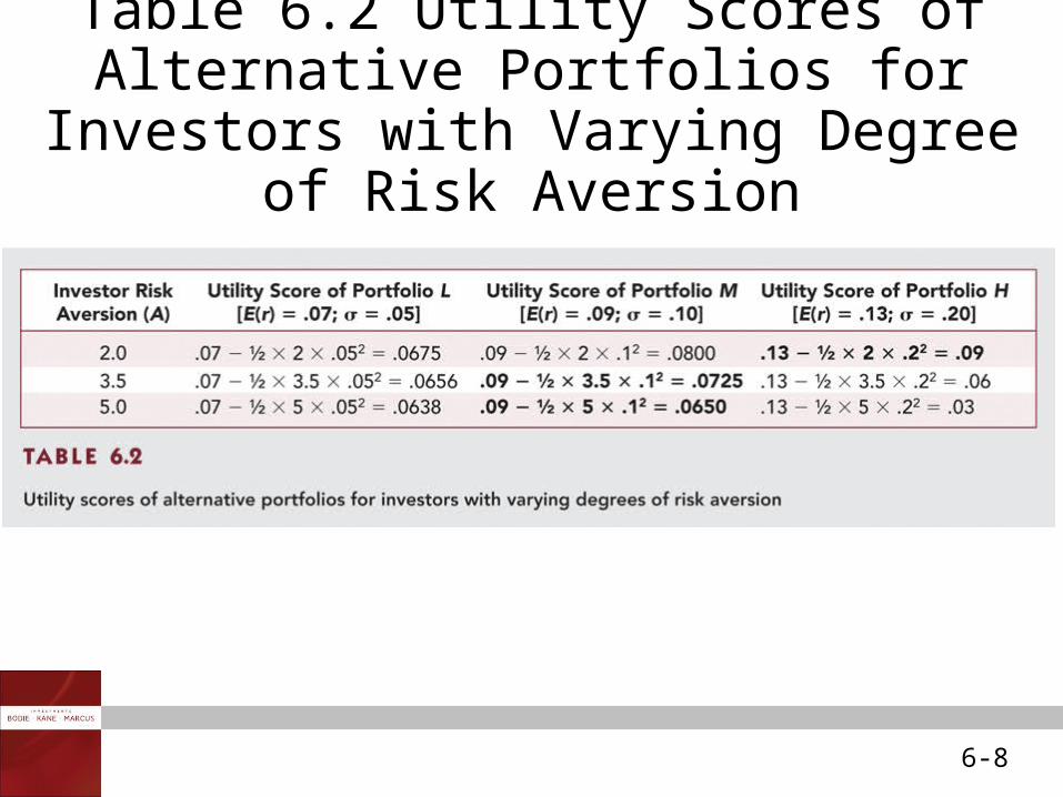
Table 6.2 Utility Scores of Alternative Portfolios for Investors with Varying

Degree of Risk Aversion

6-9

Estimating Risk Aversion

• Observe individuals’ decisions when confronted with risk

• Observe how much people are willing to pay to avoid risk

– Insurance against large losses

6-10

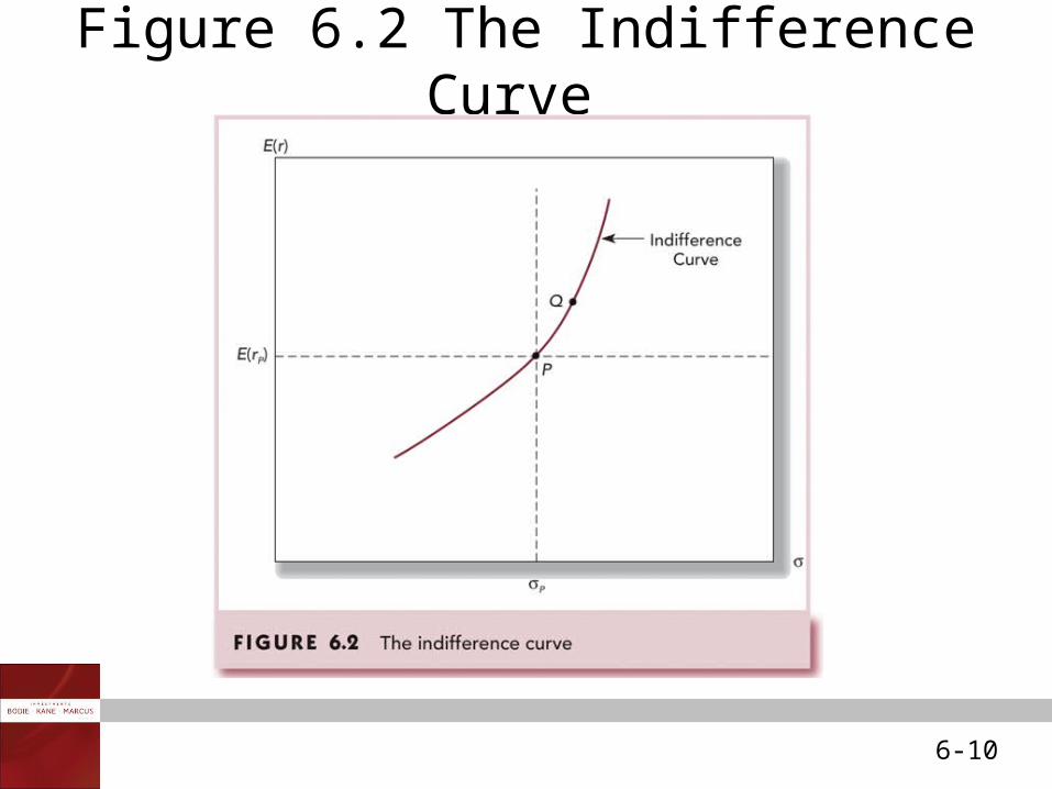
Figure 6.2 The Indifference Curve

6-11

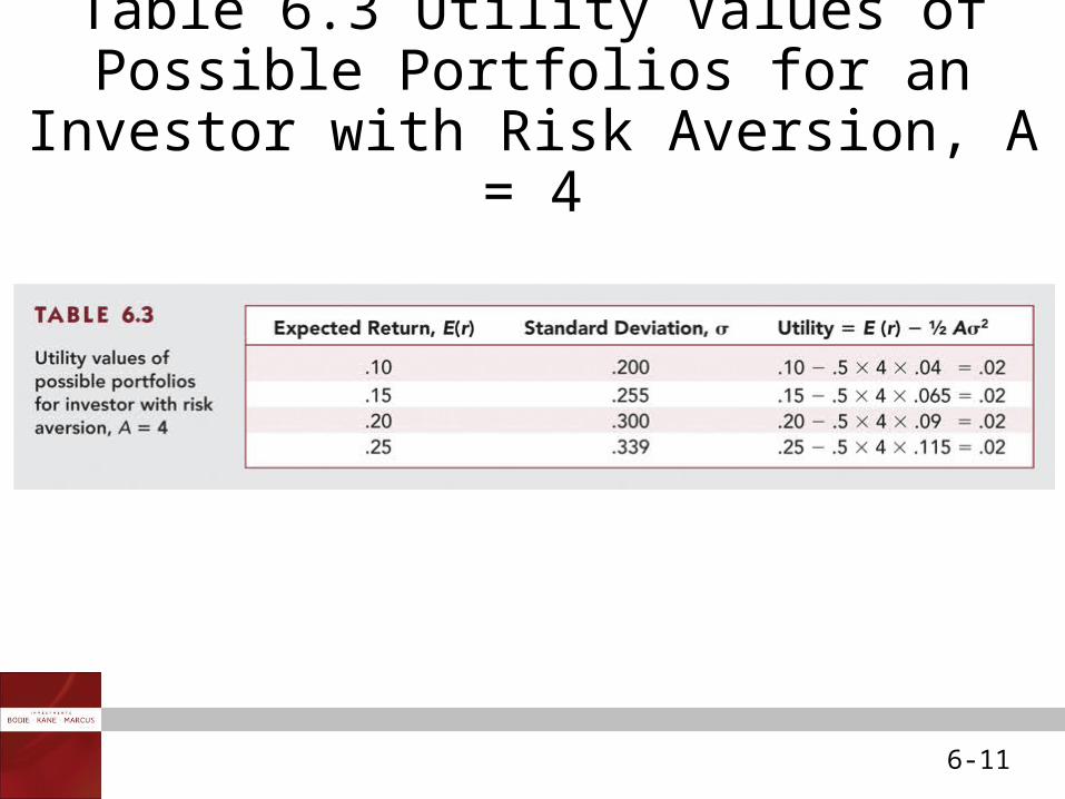
Table 6.3 Utility Values of Possible Portfolios for an Investor with Risk

Aversion, A = 4

6-12

Capital Allocation Across Risky and Risk-Free Portfolios

• Control risk

– Asset allocation choice

• Fraction of the portfolio invested in Treasury bills or other safe money market securities

6-13

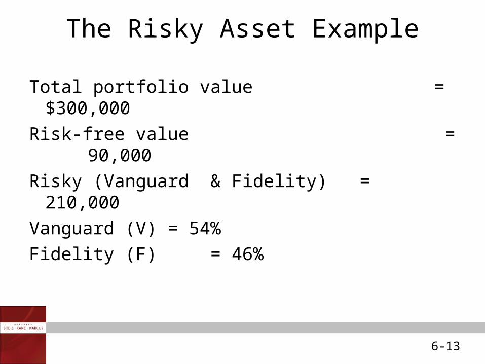
The Risky Asset Example

Total portfolio value = $300,000

Risk-free value = 90,000

Risky (Vanguard & Fidelity) = 210,000

Vanguard (V) = 54%

Fidelity (F) = 46%

6-14

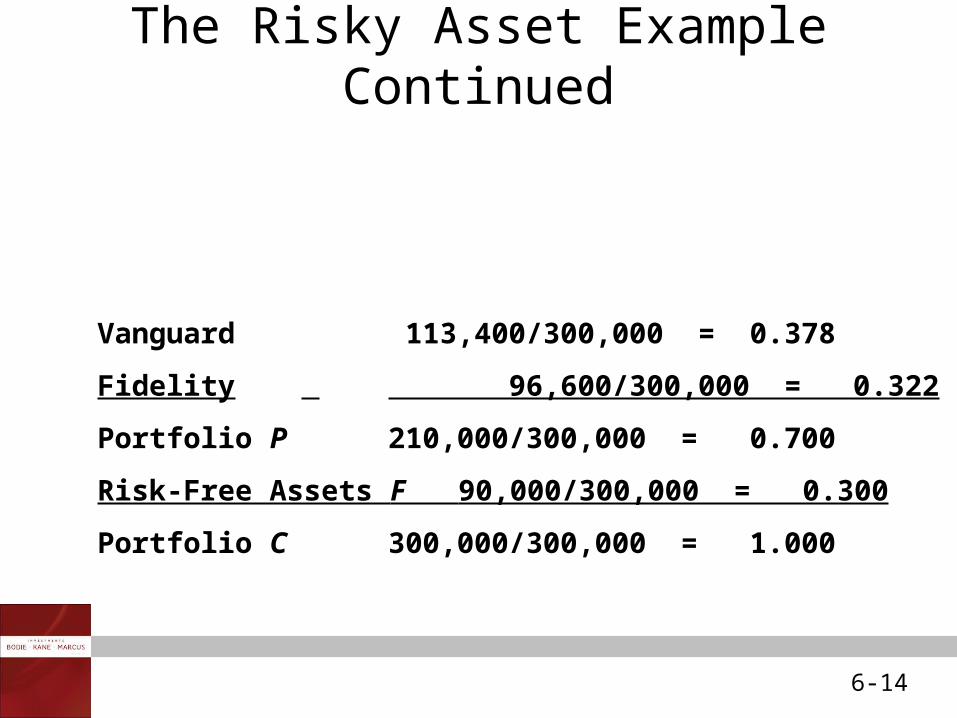
The Risky Asset Example Continued

Vanguard 113,400/300,000 = 0.378

Fidelity 96,600/300,000 = 0.322

Portfolio P 210,000/300,000 = 0.700

Risk-Free Assets F 90,000/300,000 = 0.300

Portfolio C 300,000/300,000 = 1.000

6-15

The Risk-Free Asset

• Only the government can issue default-free bonds

– Guaranteed real rate only if the duration of the bond is identical to the investor’s desire holding period

• T-bills viewed as the risk-free asset

– Less sensitive to interest rate fluctuations

6-16

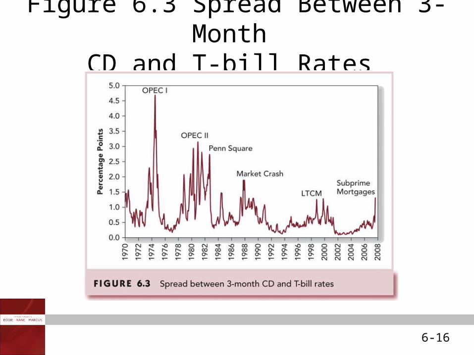
Figure 6.3 Spread Between 3-Month CD and T-bill Rates

6-17

• It’s possible to split investment funds between safe and risky assets.

• Risk free asset: proxy; T-bills

• Risky asset: stock (or a portfolio)

Portfolios of One Risky Asset and a Risk-Free Asset

6-18

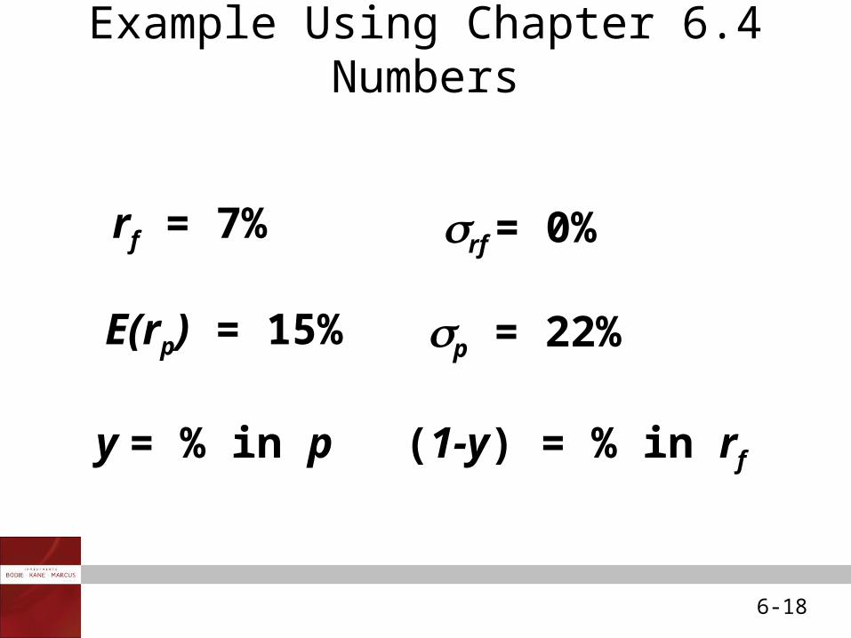
rf = 7% rf = 0%

E(rp) = 15% p = 22%

y = % in p (1-y) = % in rf

Example Using Chapter 6.4 Numbers

6-19

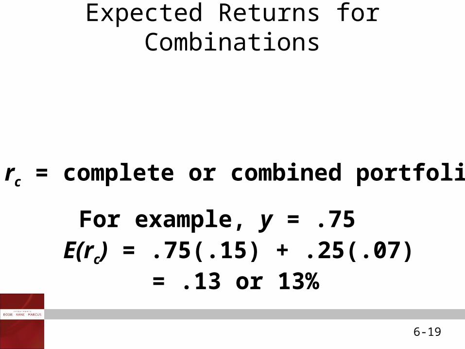
rc = complete or combined portfolio

For example, y = .75E(rc) = .75(.15) + .25(.07)

= .13 or 13%

Expected Returns for Combinations

( ) ( ) (1 )c p fE r yE r y r

6-20

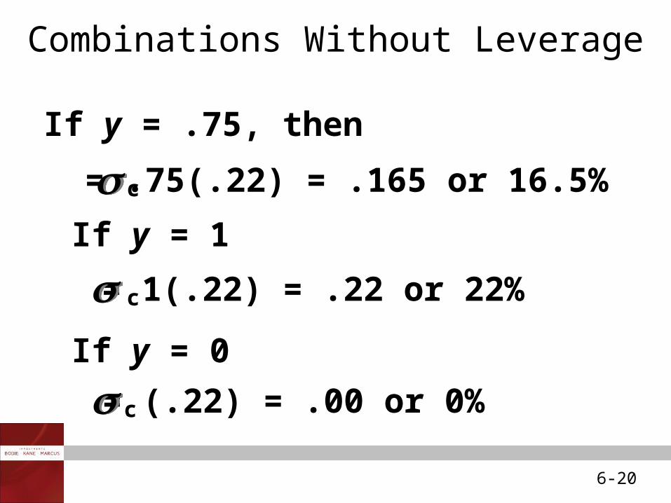
c = .75(.22) = .165 or 16.5%

If y = .75, then

c = 1(.22) = .22 or 22%

If y = 1

c = (.22) = .00 or 0%

If y = 0

Combinations Without Leverage

6-21

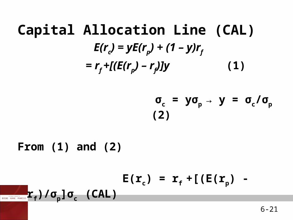
Capital Allocation Line (CAL) E(rc) = yE(rp) + (1 – y)rf

= rf +[(E(rp) – rf)]y (1)

σc = yσp → y = σc/σp (2)

From (1) and (2)

E(rc) = rf +[(E(rp) - rf)/σp]σc (CAL)

6-22

Figure 6.4 The Investment Opportunity Set with a Risky Asset and a Risk-free Asset in the

Expected Return-Standard Deviation Plane

6-23

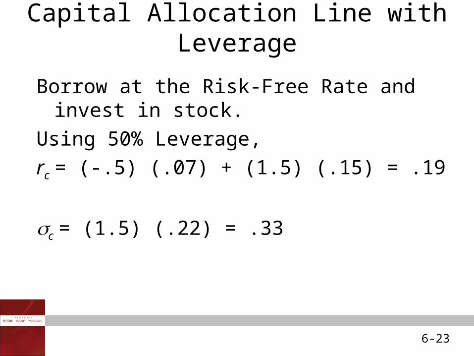
Borrow at the Risk-Free Rate and invest in stock.

Using 50% Leverage,

rc = (-.5) (.07) + (1.5) (.15) = .19

c = (1.5) (.22) = .33

Capital Allocation Line with Leverage

6-24

Figure 6.5 The Opportunity Set with Differential Borrowing and Lending Rates

6-25

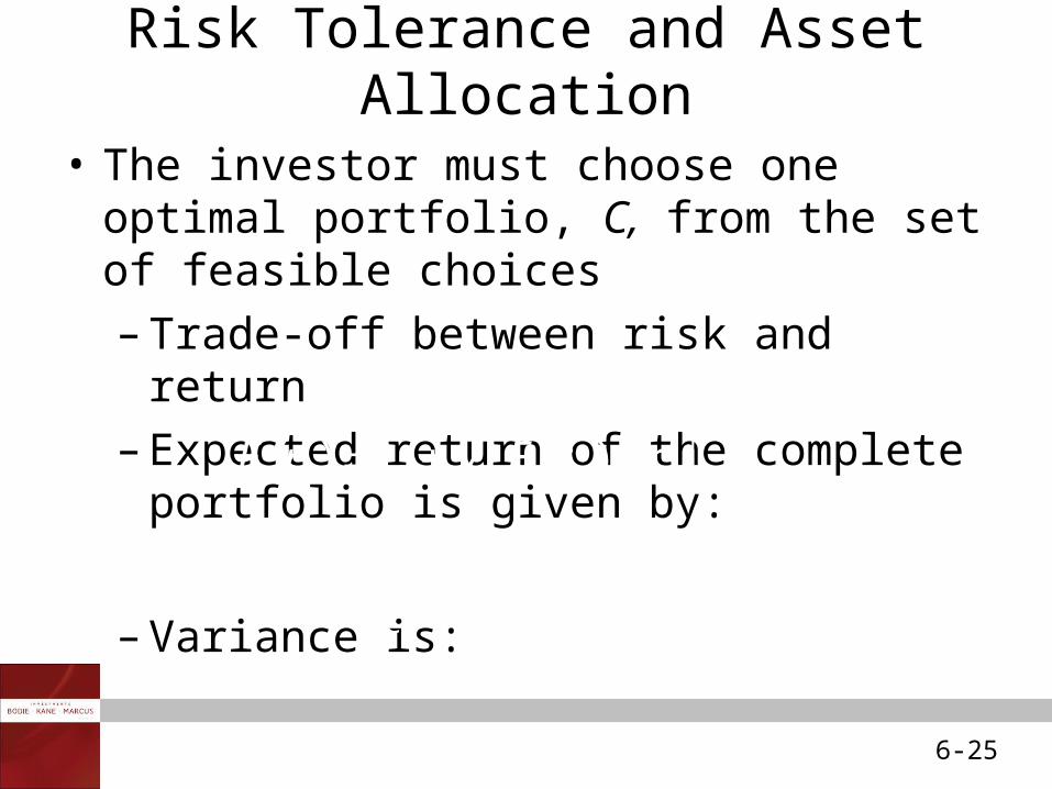
Risk Tolerance and Asset Allocation

• The investor must choose one optimal portfolio, C, from the set of feasible choices

– Trade-off between risk and return

– Expected return of the complete portfolio is given by:

– Variance is:

( ) ( )c f P fE r r y E r r

2 2 2C Py

6-26

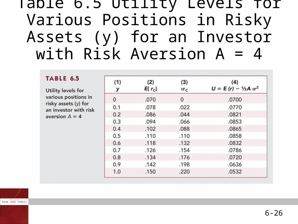
Table 6.5 Utility Levels for Various Positions in Risky Assets (y) for an Investor with Risk Aversion A = 4

6-27

Figure 6.6 Utility as a Function of Allocation to the Risky Asset, y

6-28

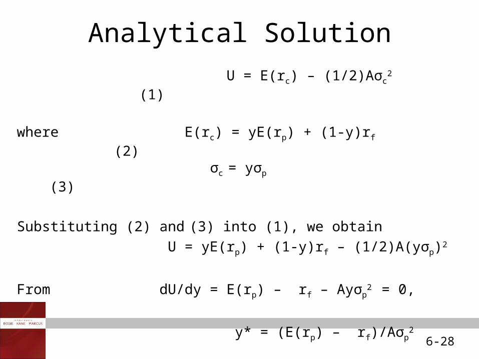
Analytical Solution

U = E(rc) – (1/2)Aσc2 (1)

where E(rc) = yE(rp) + (1-y)rf (2) σc = yσp

(3)

Substituting (2) and (3) into (1), we obtain

U = yE(rp) + (1-y)rf – (1/2)A(yσp)2

From dU/dy = E(rp) – rf – Ayσp2 = 0,

y* = (E(rp) – rf)/Aσp2

6-29

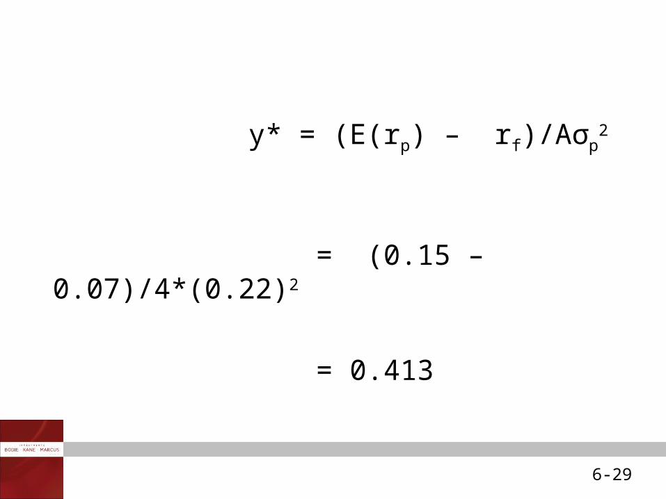
y* = (E(rp) – rf)/Aσp2

= (0.15 – 0.07)/4*(0.22)2

= 0.413

6-30

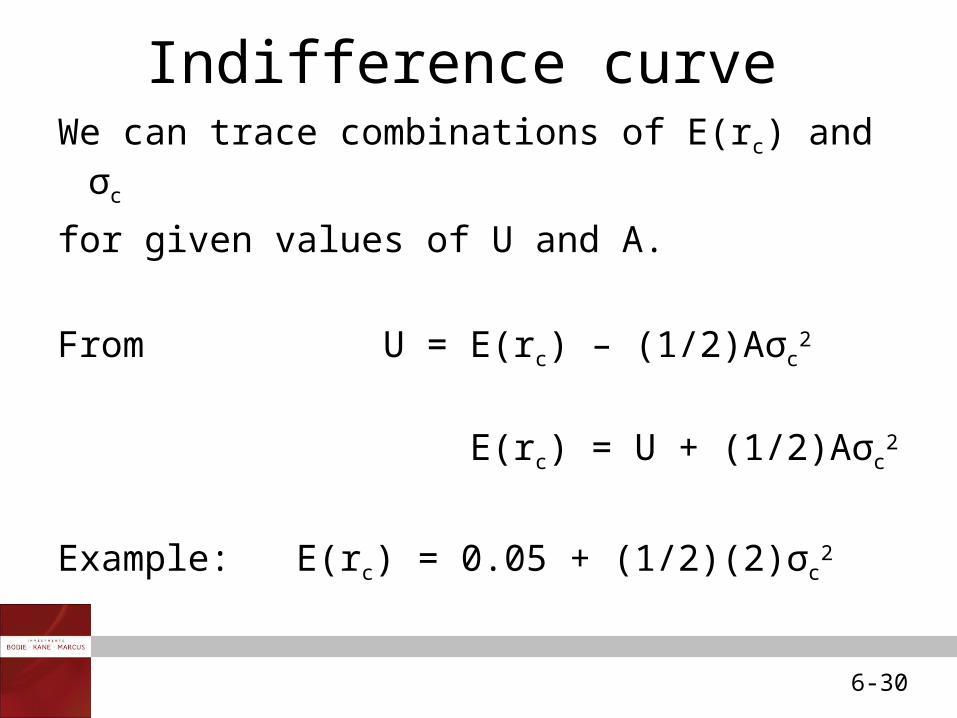
Indifference curve We can trace combinations of E(rc) and σc

for given values of U and A.

From U = E(rc) – (1/2)Aσc2

E(rc) = U + (1/2)Aσc2

Example: E(rc) = 0.05 + (1/2)(2)σc2

6-31

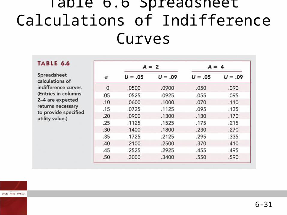
Table 6.6 Spreadsheet Calculations of Indifference Curves

6-32

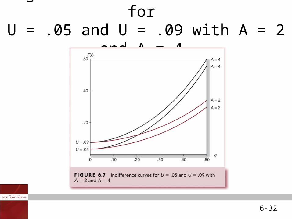
Figure 6.7 Indifference Curves for U = .05 and U = .09 with A = 2 and A = 4

6-33

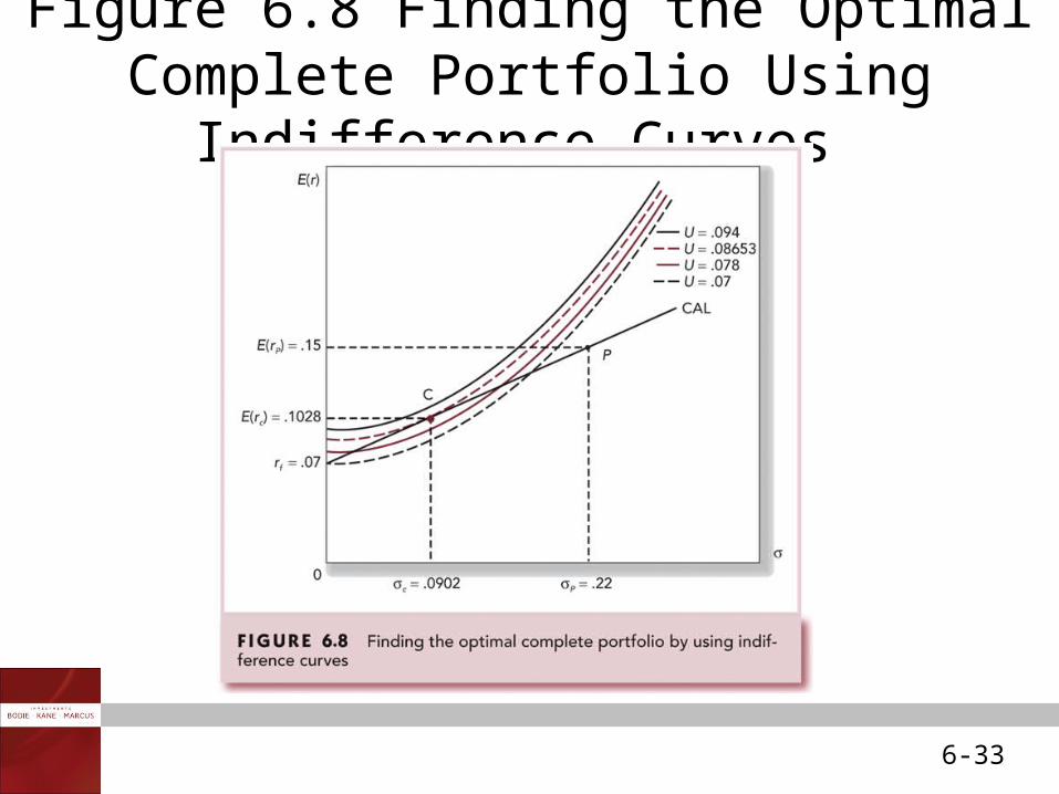
Figure 6.8 Finding the Optimal Complete Portfolio Using Indifference Curves

6-34

Passive Strategies: The Capital Market Line

• E(rc) = rf +[(E(rM) - rf)/σM]σc

• Passive strategy involves a decision that avoids any direct or indirect security analysis

• Supply and demand forces may make such a strategy a reasonable choice for many investors

6-35

Passive Strategies: The Capital Market Line Continued

• A natural candidate for a passively held risky asset would be a well-diversified portfolio of common stocks

• Because a passive strategy requires devoting no resources to acquiring information on any individual stock or group we must follow a “neutral” diversification strategy