chapter 6: models for count data - macquarie university€¦ · de jong and heller glms for...
TRANSCRIPT

De Jong and Heller GLMs for Insurance Data Chapter 6 Solutions
Chapter 6: Models for count data
6.1 Develop a statistical model for the number of claims, in the motor vehicle insurance dataset.
Frequency distribution of numclaims:
Cumulative Cumulative
numclaims Frequency Percent Frequency Percent
--------------------------------------------------------------
0 63232 93.19 63232 93.19
1 4333 6.39 67565 99.57
2 271 0.40 67836 99.97
3 18 0.03 67854 100.00
4 2 0.00 67856 100.00
As there are so few policies with numclaims>1, it is difficult to discern a trend in plotsor tables. Figure 1 shows the number of claims (logarithmic scale) plotted against vehiclevalue, with a spline curve. As this is clearly nonlinear, we use a banded form of vehiclevalue in the model, as well as vehicle value in quadratic form. (See comments and bandingscheme in Sections 4.12 and 7.3.)
0 5 10 15 20 25 30 35
Vehicle value in $10 000 units
Num
ber
of c
laim
s
12
34
0
Figure 1: Number of claims (logarithmic scale) plotted against vehicle value, with scatterplotsmoother
Using a Poisson model with log(exposure) as offset, we find that age, area, vehicle bodyand vehicle value (banded) are all significant in single regressions. Putting them together,we get the following model selection analysis:
January 9, 2008 1
De Jong and Heller GLMs for Insurance Data Chapter 6 Solutions
Model Deviance p AIC BIC
age 25415.33 6 25427.33 25482.08area 25491.52 6 25503.52 25558.27body 25469.41 13 25495.41 25614.04value (banded) 25485.33 6 25497.33 25552.08value 25484.60 2 25488.60 25506.85value + value2 25457.45 3 25463.45 25490.82age + area 25403.47 11 25425.47 25525.84age + body 25375.84 18 25411.84 25576.09age + value (banded) 25397.01 11 25419.01 25519.39area + body 25454.81 18 25490.81 25655.07area + value (banded) 25469.77 11 25491.77 25592.15body + value 25451.25 18 25487.25 25651.50age + body + value (banded) 25358.87 23 25404.87 25614.75age + area + body + value 25347.87 28 25403.87 25659.37age + body + value + value2 25329.61 20 25369.61 25552.11
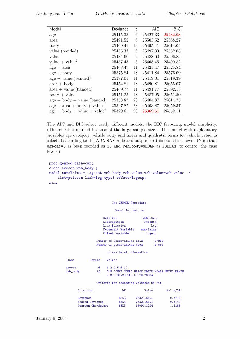
The AIC and BIC select vastly different models, the BIC favouring model simplicity.(This effect is marked because of the large sample size.) The model with explanatoryvariables age category, vehicle body and linear and quadratic terms for vehicle value, isselected according to the AIC. SAS code and output for this model is shown. (Note thatagecat=3 as been recoded as 10 and veh body=SEDAN as ZSEDAN, to control the baselevels.)
proc genmod data=car;class agecat veh_body ;model numclaims = agecat veh_body veh_value veh_value*veh_value /
dist=poisson link=log type3 offset=logexp;run;
The GENMOD Procedure
Model Information
Data Set WORK.CAR
Distribution Poisson
Link Function Log
Dependent Variable numclaims
Offset Variable logexp
Number of Observations Read 67856
Number of Observations Used 67856
Class Level Information
Class Levels Values
agecat 6 1 2 4 5 6 10
veh_body 13 BUS CONVT COUPE HBACK HDTOP MCARA MIBUS PANVN
RDSTR STNWG TRUCK UTE ZSEDA
Criteria For Assessing Goodness Of Fit
Criterion DF Value Value/DF
Deviance 68E3 25329.6101 0.3734
Scaled Deviance 68E3 25329.6101 0.3734
Pearson Chi-Square 68E3 96091.3294 1.4165
January 9, 2008 2
De Jong and Heller GLMs for Insurance Data Chapter 6 Solutions
Scaled Pearson X2 68E3 96091.3294 1.4165
Log Likelihood -17155.7039
Algorithm converged.
Analysis Of Parameter Estimates
Standard Wald 95% Chi-
Parameter DF Estimate Error Confidence Limits Square Pr > ChiSq
Intercept 1 -2.0694 0.0539 -2.1751 -1.9638 1473.09 <.0001
agecat 1 1 0.2333 0.0528 0.1297 0.3368 19.50 <.0001
agecat 2 1 0.0587 0.0430 -0.0255 0.1430 1.87 0.1718
agecat 4 1 -0.0274 0.0412 -0.1081 0.0533 0.44 0.5062
agecat 5 1 -0.2474 0.0490 -0.3435 -0.1514 25.50 <.0001
agecat 6 1 -0.2275 0.0589 -0.3430 -0.1121 14.91 0.0001
agecat 10 0 0.0000 0.0000 0.0000 0.0000 . .
veh_body BUS 1 0.8830 0.3174 0.2610 1.5050 7.74 0.0054
veh_body CONVT 1 -0.4276 0.5871 -1.5783 0.7231 0.53 0.4664
veh_body COUPE 1 0.3943 0.1186 0.1618 0.6269 11.05 0.0009
veh_body HBACK 1 -0.0170 0.0376 -0.0907 0.0567 0.20 0.6508
veh_body HDTOP 1 0.0063 0.0902 -0.1704 0.1830 0.00 0.9445
veh_body MCARA 1 0.4371 0.2603 -0.0732 0.9473 2.82 0.0932
veh_body MIBUS 1 -0.1510 0.1515 -0.4480 0.1460 0.99 0.3190
veh_body PANVN 1 0.0409 0.1240 -0.2021 0.2839 0.11 0.7416
veh_body RDSTR 1 0.3271 0.5802 -0.8100 1.4643 0.32 0.5728
veh_body STNWG 1 -0.0736 0.0423 -0.1565 0.0094 3.02 0.0822
veh_body TRUCK 1 -0.1211 0.0922 -0.3019 0.0597 1.72 0.1892
veh_body UTE 1 -0.2641 0.0661 -0.3936 -0.1346 15.97 <.0001
veh_body ZSEDA 0 0.0000 0.0000 0.0000 0.0000 . .
veh_value 1 0.2097 0.0358 0.1396 0.2798 34.40 <.0001
veh_value*veh_value 1 -0.0234 0.0056 -0.0344 -0.0124 17.43 <.0001
Scale 0 1.0000 0.0000 1.0000 1.0000
NOTE: The scale parameter was held fixed.
LR Statistics For Type 3 Analysis
Chi-
Source DF Square Pr > ChiSq
agecat 5 89.60 <.0001
veh_body 12 42.43 <.0001
veh_value 1 45.41 <.0001
veh_value*veh_value 1 28.34 <.0001
The estimated model is y ∼ P (µ), where
ln(µ) = lnn− 2.0694+0.2333x1 + . . .− 0.2275x5 (age)+0.8830x6 + . . .− 0.2641x17 (vehicle body)+0.2097x18 − 0.0234x2
18 (vehicle value) .
• The deviance (25329.6) is well below the degrees of freedom (67856-20=67836).
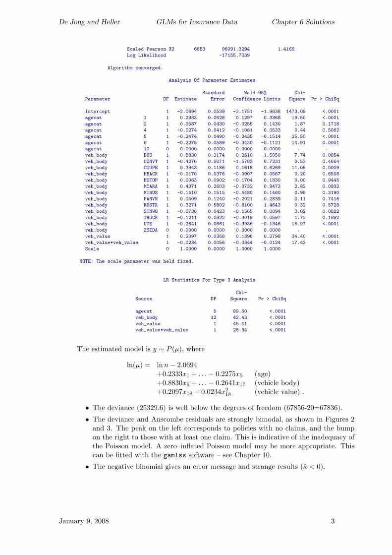
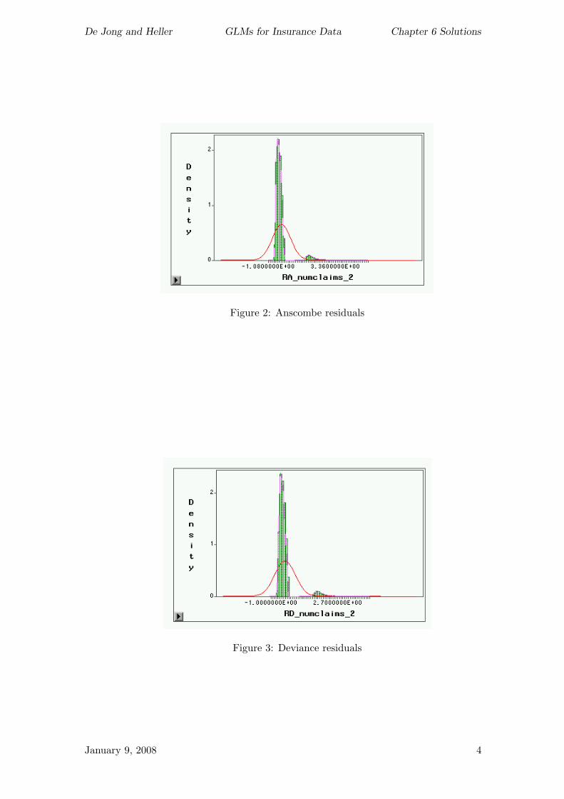
• The deviance and Anscombe residuals are strongly bimodal, as shown in Figures 2and 3. The peak on the left corresponds to policies with no claims, and the bumpon the right to those with at least one claim. This is indicative of the inadequacy ofthe Poisson model. A zero–inflated Poisson model may be more appropriate. Thiscan be fitted with the gamlss software – see Chapter 10.
• The negative binomial gives an error message and strange results (κ < 0).
January 9, 2008 3
De Jong and Heller GLMs for Insurance Data Chapter 6 Solutions
Figure 2: Anscombe residuals
Figure 3: Deviance residuals
January 9, 2008 4

De Jong and Heller GLMs for Insurance Data Chapter 6 Solutions
6.2 The SAS data file nswdeaths2002 contains all-cause mortality data for New South Wales,Australia in 2002, by age band and gender. Develop a statistical model for the number ofdeaths, using the AIC as a model selection criterion.
Death rates plotted by age and gender show a nonlinear (possibly exponential) relation-ship with age. Male death rates are higher than female death rates, at all ages. Whenlog(death rate) is plotted against age, by gender, the relationship appears linear. Also,the gender lines are roughly parallel, suggesting no age × gender interaction.
Deaths (all causes)
0
0.02
0.04
0.06
0.08
0.1
0.12
0.14
0.16
0.18
<25 25-34 35-44 45-54 55-64 65-74 75-84 85+
Age group
Rat
e Male
Female
Deaths (all causes)
-4
-3.5
-3
-2.5
-2
-1.5
-1
-0.5
0<25 25-34 35-44 45-54 55-64 65-74 75-84 85+
Age group
log
(Dea
th r
ate)
MaleFemale
Model for deaths (all causes) Start with a Poisson response distribution with loglink, and using log(population) as offset:
y ∼ P (µ) , ln µ = ln n + x′β
where y is the number of deaths due to all causes in an age-gender category.
The model with age (categorical) and gender has deviance of 261.3 on 7 d.f., indicat-ing overdispersion. (Check that no other Poisson model gives an adequate deviance.)Negative binomial model:
y ∼ NB(µ, k) , ln µ = lnn + x′β .
Models using age as a categorical covariate, and as a continuous covariate (with the mid-points of the age bands as the age values) are compared. Using the AIC, the preferredmodel has gender, age as a quadratic, and an age–gender interaction term.
Model ∆ df ` p AIC
age (cat) 16.3 8 344904.7 8 -689793.4gender 21.1 14 344872.1 2 -689740.3age (cat) + gender 17.2 7 344921.6 9 -689825.2age (cont) 16.5 14 344899.3 2 -689794.6age (cont) + gender 16.3 13 344903.8 3 -689801.6age (cont) + age (cont)2 + gender 16.8 12 344919.0 4 -689830.0age (cont) + age (cont)2 + gender +
age (cont)×gender 17.6 11 344923.0 5 -689836.0age (cont) + age (cont)2 + gender +
age (cont)×gender + age (cont)2×gender 17.6 10 344923.5 6 -689835.0
January 9, 2008 5
De Jong and Heller GLMs for Insurance Data Chapter 6 Solutions
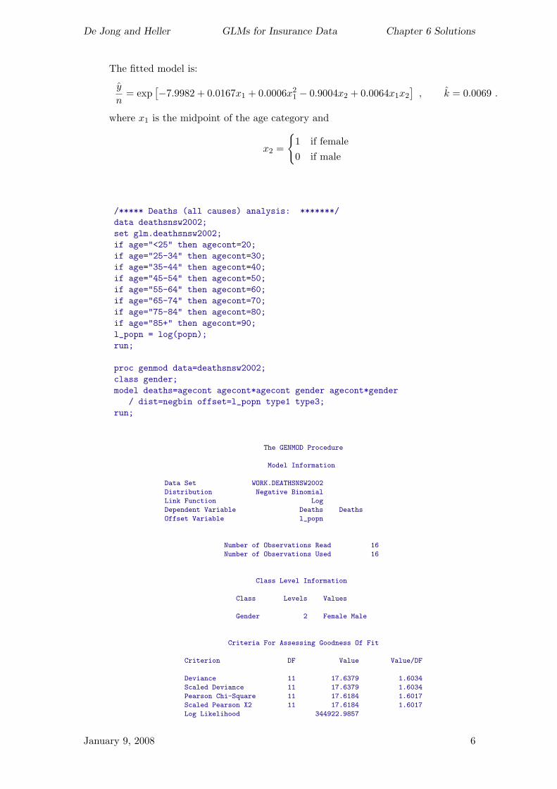
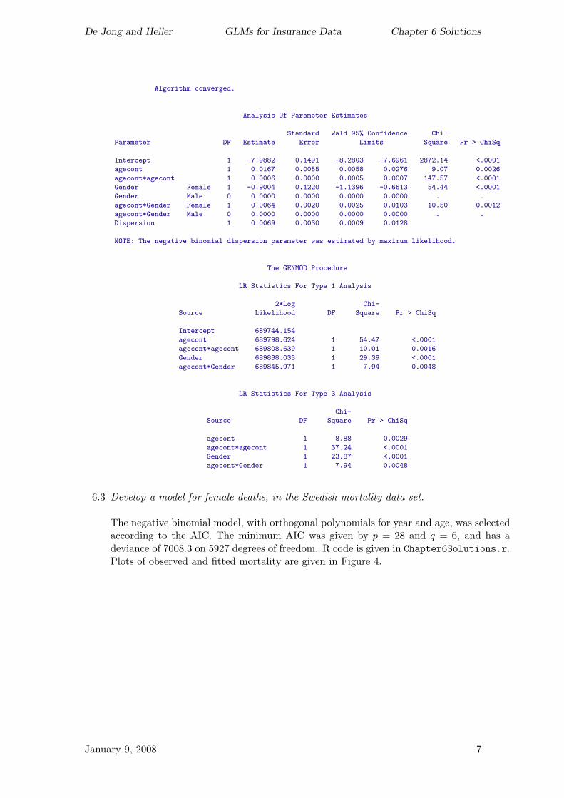
The fitted model is:
y
n= exp
[−7.9982 + 0.0167x1 + 0.0006x21 − 0.9004x2 + 0.0064x1x2
], k = 0.0069 .
where x1 is the midpoint of the age category and
x2 =
{1 if female0 if male
/***** Deaths (all causes) analysis: *******/data deathsnsw2002;set glm.deathsnsw2002;if age="<25" then agecont=20;if age="25-34" then agecont=30;if age="35-44" then agecont=40;if age="45-54" then agecont=50;if age="55-64" then agecont=60;if age="65-74" then agecont=70;if age="75-84" then agecont=80;if age="85+" then agecont=90;l_popn = log(popn);run;
proc genmod data=deathsnsw2002;class gender;model deaths=agecont agecont*agecont gender agecont*gender
/ dist=negbin offset=l_popn type1 type3;run;
The GENMOD Procedure
Model Information
Data Set WORK.DEATHSNSW2002
Distribution Negative Binomial
Link Function Log
Dependent Variable Deaths Deaths
Offset Variable l_popn
Number of Observations Read 16
Number of Observations Used 16
Class Level Information
Class Levels Values
Gender 2 Female Male
Criteria For Assessing Goodness Of Fit
Criterion DF Value Value/DF
Deviance 11 17.6379 1.6034
Scaled Deviance 11 17.6379 1.6034
Pearson Chi-Square 11 17.6184 1.6017
Scaled Pearson X2 11 17.6184 1.6017
Log Likelihood 344922.9857
January 9, 2008 6
De Jong and Heller GLMs for Insurance Data Chapter 6 Solutions
Algorithm converged.
Analysis Of Parameter Estimates
Standard Wald 95% Confidence Chi-
Parameter DF Estimate Error Limits Square Pr > ChiSq
Intercept 1 -7.9882 0.1491 -8.2803 -7.6961 2872.14 <.0001
agecont 1 0.0167 0.0055 0.0058 0.0276 9.07 0.0026
agecont*agecont 1 0.0006 0.0000 0.0005 0.0007 147.57 <.0001
Gender Female 1 -0.9004 0.1220 -1.1396 -0.6613 54.44 <.0001
Gender Male 0 0.0000 0.0000 0.0000 0.0000 . .
agecont*Gender Female 1 0.0064 0.0020 0.0025 0.0103 10.50 0.0012
agecont*Gender Male 0 0.0000 0.0000 0.0000 0.0000 . .
Dispersion 1 0.0069 0.0030 0.0009 0.0128
NOTE: The negative binomial dispersion parameter was estimated by maximum likelihood.
The GENMOD Procedure
LR Statistics For Type 1 Analysis
2*Log Chi-
Source Likelihood DF Square Pr > ChiSq
Intercept 689744.154
agecont 689798.624 1 54.47 <.0001
agecont*agecont 689808.639 1 10.01 0.0016
Gender 689838.033 1 29.39 <.0001
agecont*Gender 689845.971 1 7.94 0.0048
LR Statistics For Type 3 Analysis
Chi-
Source DF Square Pr > ChiSq
agecont 1 8.88 0.0029
agecont*agecont 1 37.24 <.0001
Gender 1 23.87 <.0001
agecont*Gender 1 7.94 0.0048
6.3 Develop a model for female deaths, in the Swedish mortality data set.
The negative binomial model, with orthogonal polynomials for year and age, was selectedaccording to the AIC. The minimum AIC was given by p = 28 and q = 6, and has adeviance of 7008.3 on 5927 degrees of freedom. R code is given in Chapter6Solutions.r.Plots of observed and fitted mortality are given in Figure 4.
January 9, 2008 7

De Jong and Heller GLMs for Insurance Data Chapter 6 Solutions
1960
19701980
19902000
0
20
40
60
80
100
−10
−8
−6
−4
−2
0
Year
Age
Log
deat
h ra
te
1960
19701980
19902000
0
20
40
60
80
100
−10
−8
−6
−4
−2
0
Year
Age
Log
deat
h ra
te
Figure 4: Observed and fitted Swedish female death rates
January 9, 2008 8