chapter 6 minds: architecture & design

Chapter 6

MINDS: ARCHITECTURE & DESIGN

Varun Chandola, Eric Eilertson, Levent Ert�oz, Gy�orgy Simon and Vipin KumarDepartment of Computer ScienceUniversity of Minnesota{chandola,eric,ertoz,gsimon,kumar}@cs.umn.edu

Abstract This chapter provides an overview of the Minnesota Intrusion Detection System(MINDS), which uses a suite of data mining based algorithms to address differentaspects of cyber security. The various components of MINDS such as the scandetector, anomaly detector and the pro�ling module detect different types of at-tacks and intrusions on a computer network. The scan detector aims at detectingscans which are the percusors to any network attack. The anomaly detection al-gorithm is very effective in detecting behavioral anomalies in the network traf�cwhich typically translate to malicious activities such as denial-of-service (DoS)traf�c, worms, policy violations and inside abuse. The pro�ling module helps anetwork analyst to understand the characteristics of the network traf�c and detectany deviations from the normal pro�le. Our analysis shows that the intrusionsdetected by MINDS are complementary to those of traditional signature based sys-tems, such as SNORT, which implies that they both can be combined to increaseoverall attack coverage. MINDS has shown great operational success in detectingnetwork intrusions in two live deployments at the University of Minnesota andas a part of the Interrogator architecture at the US Army Research Lab�s Centerfor Intrusion Monitoring and Protection (ARL-CIMP).

Keywords: network intrusion detection, anomaly detection, summarization, pro�ling, scandetection

The conventional approach to securing computer systems against cyber threatsis to design mechanisms such as �rewalls, authentication tools, and virtual pri-vate networks that create a protective shield. However, these mechanisms almostalways have vulnerabilities. They cannot ward off attacks that are continuallybeing adapted to exploit system weaknesses, which are often caused by carelessdesign and implementation �aws. This has created the need for intrusion detec-tion [6], security technology that complements conventional security approachesby monitoring systems and identifying computer attacks.

84 MINDS: Architecture & Design

Traditional intrusion detection methods are based on human experts' extensiveknowledge of attack signatures which are character strings in a message�s pay-load that indicate malicious content. Signatures have several limitations. Theycannot detect novel attacks, because someone must manually revise the signaturedatabase beforehand for each new type of intrusion discovered. Once someonediscovers a new attack and develops its signature, deploying that signature isoften delayed. These limitations have led to an increasing interest in intrusiondetection techniques based on data mining [12, 22, 2].

This chapter provides an overview of the Minnesota Intrusion Detection Sys-tem (MINDS1) which is a suite of different data mining based techniques to addressdifferent aspects of cyber security. In Section 1 we will discuss the overall archi-tecture of MINDS. In the subsequent sections we will brie�y discuss the differentcomponents of MINDS which aid in intrusion detection using various data miningapproaches.

1. MINDS - Minnesota INtrusion Detection System

DataCaptureDevice

Storage

Network

FilteringFeature

ExtractionKnown Attack

Detection

AnomalyDetection

AnomalyScores

AssociationPatternAnalysis

Summary ofanomalies

Detected knownattacks

Analyst

Labels

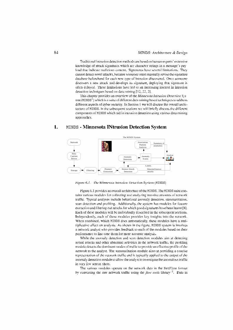
The MINDS System

Figure 6.1. The Minnesota Intrusion Detection System (MINDS)

Figure 6.1 provides an overall architecture of the MINDS. The MINDS suite con-tains various modules for collecting and analyzing massive amounts of networktraf�c. Typical analyses include behavioral anomaly detection, summarization,scan detection and pro�ling. Additionally, the system has modules for featureextraction and �ltering out attacks for which good signatures have been learnt [8].Each of these modules will be individually described in the subsequent sections.Independently, each of these modules provides key insights into the network.When combined, which MINDS does automatically, these modules have a mul-tiplicative affect on analysis. As shown in the �gure, MINDS system is involvesa network analyst who provides feedback to each of the modules based on theirperformance to �ne tune them for more accurate analysis.

While the anomaly detection and scan detection modules aim at detectingactual attacks and other abnormal activities in the network traf�c, the pro�lingmodule detects the dominant modes of traf�c to provide an effective pro�le of thenetwork to the analyst. The summarization module aims at providing a conciserepresentation of the network traf�c and is typically applied to the output of theanomaly detection module to allow the analyst to investigate the anomalous traf�cin very few screen-shots.

The various modules operate on the network data in the NetFlow formatby converting the raw network traf�c using the �ow-tools library 2. Data in

Anomaly Detection 85

NetFlow format is a collection of records, where each record corresponds to aunidirectional �ow of packets within a session. Thus each session (also referred toas a connection) between two hosts comprises of two �ows in opposite directions.These records are highly compact containing summary information extractedprimarily from the packet headers. This information includes source IP, sourceport, destination IP, destination port, number of packets, number of bytes andtimestamp. Various modules extract more features from these basic features andapply data mining algorithms on the data set de�ned over the set of basic as wellas derived features.

MINDS is deployed at the University of Minnesota, where several hundredmillion network �ows are recorded from a network of more than 40,000 computersevery day. MINDS is also part of the Interrogator [15] architecture at the US ArmyResearch Lab�s Center for Intrusion Monitoring and Protection (ARL-CIMP),where analysts collect and analyze network traf�c from dozens of Departmentof Defense sites [7]. MINDS is enjoying great operational success at both sites,routinely detecting brand new attacks that signature-based systems could not havefound. Additionally, it often discovers rogue communication channels and theex�ltration of data that other widely used tools such as SNORT [19] have haddif�culty identifying.

2. Anomaly DetectionAnomaly detection approaches build models of normal data and detect de-

viations from the normal model in observed data. Anomaly detection appliedto intrusion detection and computer security has been an active area of researchsince it was originally proposed by Denning [6]. Anomaly detection algorithmshave the advantage that they can detect emerging threats and attacks (which do nothave signatures or labeled data corresponding to them) as deviations from normalusage. Moreover, unlike misuse detection schemes (which build classi�cationmodels using labeled data and then classify an observation as normal or attack),anomaly detection algorithms do not require an explicitly labeled training dataset, which is very desirable, as labeled data is dif�cult to obtain in a real networksetting.

The MINDS anomaly detection module is a local outlier detection techniquebased on the local outlier factor (LOF) algorithm [3]. The LOF algorithm iseffective in detecting outliers in data which has regions of varying densities(such as network data) and has been found to provide competitive performancefor network traf�c analysis[13].

The input to the anomaly detection algorithm is NetFlow data as described inthe previous section. The algorithm extracts 8 derived features for each �ow [8].Figure 6.2 lists the set of features which are used to represent a network �ow inthe anomaly detection algorithm. Note that all of these features are either presentin the NetFlow data or can be extracted from it without requiring to look at thepacket contents.

Applying the LOF algorithm to network data involves computation of similar-ity between a pair of �ows that contain a combination of categorical and numericalfeatures. The anomaly detection algorithm uses a novel data-driven technique forcalculating the distance between points in a high-dimensional space. Notably,this technique enables meaningful calculation of the similarity between recordscontaining a mixture of categorical and numerical features shown in Figure 6.2.


BasicSource IPSource PortDestination IPDestination PortProtocolDurationPackets SentBytes per Packet Sent

Derived (Time-window Based)count-dest Number of �ows to unique destina-

tion IP addresses inside the networkin the last T seconds from the samesource

count-src Number of �ows from uniquesource IP addresses inside the net-work in the last T seconds to thesame destination

count-serv-src Number of �ows from the source IPto the same destination port in thelast T seconds

count-serv-dest Number of �ows to the destinationIP address using same source port inthe last T seconds

Derived (Connection Based)count-dest-conn Number of �ows to unique destina-

tion IP addresses inside the networkin the last N �ows from the samesource

count-src-conn Number of �ows from uniquesource IP addresses inside the net-work in the lastN �ows to the samedestination

count-serv-src-conn Number of �ows from the source IPto the same destination port in thelast N �ows

count-serv-dest-conn Number of �ows to the destinationIP address using same source port inthe last N �ows

Figure 6.2. The set of features used by the MINDS anomaly detection algorithm

LOF requires the neighborhood around all data points be constructed. Thisinvolves calculating pairwise distances between all data points, which is anO(n2)process, which makes it computationally infeasible for a large number of datapoints. To address this problem, we sample a training set from the data andcompare all data points to this small set, which reduces the complexity toO(n∗m)where n is the size of the data and m is the size of the sample. Apart fromachieving computational ef�ciency, sampling also improves the quality of theanomaly detector output. The normal �ows are very frequent and the anomalous�ows are rare in the actual data. Hence the training data (which is drawn uniformlyfrom the actual data) is more likely to contain several similar normal �ows andfar less likely to contain a substantial number of similar anomalous �ows. Thusan anomalous �ow will be unable to �nd similar anomalous neighbors in thetraining data and will have a high LOF score. The normal �ows on the other handwill �nd enough similar normal �ows in the training data and will have a lowLOF score.

Summarization 87

Thus the MINDS anomaly detection algorithm takes as input a set of network�ows3 and extracts a random sample as the training set. For each �ow in theinput data, it then computes its nearest neighbors in the training set. Using thenearest neighbor set it then computes the LOF score (referred to as the AnomalyScore) for that particular �ow. The �ows are then sorted based on their anomalyscores and presented to the analyst in a format described in the next section.

Output of Anomaly Detection Algorithm. The output of theMINDS anomaly detector is in plain text format with each input �ow described ina single line. The �ows are sorted according to their anomaly scores such that thetop �ow corresponds to the most anomalous �ow (and hence most interesting forthe analyst) according to the algorithm. For each �ow, its anomaly score and thebasic features describing that �ow are displayed. Additionally, the contributionof each feature towards the anomaly score is also shown. The contribution of aparticular feature signi�es how different that �ow was from its neighbors in thatfeature. This allows the analyst to understand the cause of the anomaly in termsof these features.

Table 6.1 is a screen-shot of the output generated by the MINDS anomalydetector from its live operation at the University of Minnesota. This output isfor January 25, 2003 data which is one day after the Slammer worm hit theInternet. All the top 23 �ows shown in Table 6.1 actually correspond to theworm related traf�c generated by an external host to different U of M machineson destination port 1434 (which corresponds to the Slammer worm). The �rstentry in each line denotes the anomaly score of that �ow. The very high anomalyscore for the top �ows(the normal �ows are assigned a score close to 1), illustratesthe strength of the anomaly detection module in separating the anomalous traf�cfrom the normal. Entries 2�7 show the basic features for each �ow while the lastentry lists all the features which had a signi�cant contribution to the anomalyscore. Thus we observe that the anomaly detector detects all worm related traf�cas the top anomalies. The contribution vector for each of the �ow signi�es thatthese anomalies were caused due to the feature � count src conn. The anomalydue to this particular feature translates to the fact that the external source wastalking to an abnormally high number of inside hosts during a window of certainnumber of connections.

Table 6.2 shows another output screen-shot from the University of Minnesotanetwork traf�c for January 26, 2003 data (48 hours after the Slammer wormhit the Internet). By this time, the effect of the worm attack was reduced due topreventive measures taken by the network administrators. Table 6.2 shows thetop 32 anomalous �ows as ranked by the anomaly detector. Thus while most ofthe top anomalous �ows still correspond to the worm traf�c originating from anexternal host to different U of M machines on destination port 1434, there are twoother type of anomalous �ows which are highly ranked by the anomaly detector

1 Anomalous �ows that correspond to a ping scan by an external host (Bold rows in Table6.2)

2 Anomalous �ows corresponding to U of M machines connecting to half-life game servers(Italicized rows in Table 6.2)

88 MINDS: Architecture & Designsc

ore

srcIP

sPor

tds

tIP

dPor

tpr

oto

pkts

bytes

cont

ribut

ion

2082

6.69

128.

171.

X.62

1042

160.

94.X

.101

1434

tcp[0

,2)

[387

,126

4)countsrcconn

=1.

0020

344.

8312

8.17

1.X.

6210

4216

0.94

.X.1

1014

34tcp

[0,2

)[3

87,1

264)

countsrcconn

=1.

0019

295.

8212

8.17

1.X.

6210

4216

0.94

.X.7

914

34tcp

[0,2

)[3

87,1

264)

countsrcconn

=1.

0018

717.

112

8.17

1.X.

6210

4216

0.94

.X.4

714

34tcp

[0,2

)[3

87,1

264)

countsrcconn

=1.

0018

147.

1612

8.17

1.X.

6210

4216

0.94

.X.1

8314

34tcp

[0,2

)[3

87,1

264)

countsrcconn

=1.

0017

484.

1312

8.17

1.X.

6210

4216

0.94

.X.1

0114

34tcp

[0,2

)[3

87,1

264)

countsrcconn

=1.

0016

715.

6112

8.17

1.X.

6210

4216

0.94

.X.1

6614

34tcp

[0,2

)[3

87,1

264)

countsrcconn

=1.

0015

973.

2612

8.17

1.X.

6210

4216

0.94

.X.1

0214

34tcp

[0,2

)[3

87,1

264)

countsrcconn

=1.

0013

084.

2512

8.17

1.X.

6210

4216

0.94

.X.5

414

34tcp

[0,2

)[3

87,1

264)

countsrcconn

=1.

0012

797.

7312

8.17

1.X.

6210

4216

0.94

.X.1

8914

34tcp

[0,2

)[3

87,1

264)

countsrcconn

=1.

0012

428.

4512

8.17

1.X.

6210

4216

0.94

.X.2

4714

34tcp

[0,2

)[3

87,1

264)

countsrcconn

=1.

0011

245.

2112

8.17

1.X.

6210

4216

0.94

.X.5

814

34tcp

[0,2

)[3

87,1

264)

countsrcconn

=1.

0093

27.9

812

8.17

1.X.

6210

4216

0.94

.X.1

3514

34tcp

[0,2

)[3

87,1

264)

countsrcconn

=1.

0074

68.5

212

8.17

1.X.

6210

4216

0.94

.X.9

114

34tcp

[0,2

)[3

87,1

264)

countsrcconn

=1.

0054

89.6

912

8.17

1.X.

6210

4216

0.94

.X.3

014

34tcp

[0,2

)[3

87,1

264)

countsrcconn

=1.

0050

70.5

128.

171.

X.62

1042

160.

94.X

.233

1434

tcp[0

,2)

[387

,126

4)countsrcconn

=1.

0045

58.7

212

8.17

1.X.

6210

4216

0.94

.X.1

1434

tcp[0

,2)

[387

,126

4)countsrcconn

=1.

0042

25.0

912

8.17

1.X.

6210

4216

0.94

.X.1

4314

34tcp

[0,2

)[3

87,1

264)

countsrcconn

=1.

0041

70.7

212

8.17

1.X.

6210

4216

0.94

.X.2

2514

34tcp

[0,2

)[3

87,1

264)

countsrcconn

=1.

0029

37.4

212

8.17

1.X.

6210

4216

0.94

.X.7

514

34tcp

[0,2

)[3

87,1

264)

countsrcconn

=1.

0024

58.6

112

8.17

1.X.

6210

4216

0.94

.X.1

5014

34tcp

[0,2

)[3

87,1

264)

countsrcconn

=1.

0011

16.4

112

8.17

1.X.

6210

4216

0.94

.X.2

5514

34tcp

[0,2

)[3

87,1

264)

countsrcconn

=1.

0010

35.1

712

8.17

1.X.

6210

4216

0.94

.X.5

014

34tcp

[0,2

)[3

87,1

264)

countsrcconn

=1.

00

Tabl

e6.1

.Sc

reen

-shot

ofMINDS

anom

alyde

tectio

nalg

orith

mou

tput

forU

ofM

data

forJ

anuary25,2003

.The

third

octet

ofth

eIPs

isan

onym

ized

forp

rivac

ypr

eser

vatio

n.

Summarization 89sc

ore

srcIP

sPor

tds

tIP

dPor

tpr

oto

pkts

bytes

cont

ribut

ion

3767

4.69

63.1

50.X

.253

1161

128.

101.

X.29

1434

tcp[0

,2)

[0,1

829)

countsrcconn

=0.

66,countdstconn

=0.

3426

676.

6263

.150

.X.2

5311

6116

0.94

.X.1

3414

34tcp

[0,2

)[0

,182

9)countsrcconn

=0.

66,countdstconn

=0.

3424

323.

5563

.150

.X.2

5311

6112

8.10

1.X.

185

1434

tcp[0

,2)

[0,1

829)

countsrcconn

=0.

66,countdstconn

=0.

3421

169.

4963

.150

.X.2

5311

6116

0.94

.X.7

114

34tcp

[0,2

)[0

,182

9)countsrcconn

=0.

66,countdstconn

=0.

3419

525.

3163

.150

.X.2

5311

6116

0.94

.X.1

914

34tcp

[0,2

)[0

,182

9)countsrcconn

=0.

66,countdstconn

=0.

3419

235.

3963

.150

.X.2

5311

6116

0.94

.X.8

014

34tcp

[0,2

)[0

,182

9)countsrcconn

=0.

66,countdstconn

=0.

3417

679.

163

.150

.X.2

5311

6116

0.94

.X.2

2014

34tcp

[0,2

)[0

,182

9)countsrcconn

=0.

66,countdstconn

=0.

3481

83.5

863

.150

.X.2

5311

6112

8.10

1.X.

108

1434

tcp[0

,2)

[0,1

829)

countsrcconn

=0.

66,countdstconn

=0.

3471

42.9

863

.150

.X.2

5311

6112

8.10

1.X.

223

1434

tcp[0

,2)

[0,1

829)

countsrcconn

=0.

66,countdstconn

=0.

3451

39.0

163

.150

.X.2

5311

6112

8.10

1.X.

142

1434

tcp[0

,2)

[0,1

829)

countsrcconn

=0.

66,countdstconn

=0.

3440

48.4

914

2.15

0.X.

101

012

8.10

1.X.

127

2048

icmp

[2,4

)[0

,182

9)countsrcconn

=0.

69,countdstconn

=0.

3140

08.3

520

0.25

0.Z.

2027

016

128.

101.

X.11

646

29tc

p[2

,4)

[0,1

829)

countdst

=1.

0036

57.2

320

2.17

5.Z.

237

2701

612

8.10

1.X.

116

4148

tcp

[2,4

)[0

,182

9)countdst

=1.

0034

50.9

63.1

50.X

.253

1161

128.

101.

X.62

1434

tcp[0

,2)

[0,1

829)

countsrcconn

=0.

66,countdstconn

=0.

3433

27.9

863

.150

.X.2

5311

6116

0.94

.X.2

2314

34tcp

[0,2

)[0

,182

9)countsrcconn

=0.

66,countdstconn

=0.

3427

96.1

363

.150

.X.2

5311

6112

8.10

1.X.

241

1434

tcp[0

,2)

[0,1

829)

countsrcconn

=0.

66,countdstconn

=0.

3426

93.8

814

2.15

0.X.

101

012

8.10

1.X.

168

2048

icmp

[2,4

)[0

,182

9)countsrcconn

=0.

69,countdstconn

=0.

3126

83.0

563

.150

.X.2

5311

6116

0.94

.X.4

314

34tcp

[0,2

)[0

,182

9)countsrcconn

=0.

66,countdstconn

=0.

3424

44.1

614

2.15

0.X.

236

012

8.10

1.X.

240

2048

icmp

[2,4

)[0

,182

9)countsrcconn

=0.

69,countdstconn

=0.

3123

85.4

214

2.15

0.X.

101

012

8.10

1.X.

4520

48icm

p[0

,2)

[0,1

829)

countsrcconn

=0.

69,countdstconn

=0.

3121

14.4

163

.150

.X.2

5311

6116

0.94

.X.1

8314

34tcp

[0,2

)[0

,182

9)countsrcconn

=0.

66,countdstconn

=0.

3420

57.1

514

2.15

0.X.

101

012

8.10

1.X.

161

2048

icmp

[0,2

)[0

,182

9)countsrcconn

=0.

69,countdstconn

=0.

3119

19.5

414

2.15

0.X.

101

012

8.10

1.X.

9920

48icm

p[2

,4)

[0,1

829)

countsrcconn

=0.

69,countdstconn

=0.

3116

34.3

814

2.15

0.X.

101

012

8.10

1.X.

219

2048

icmp

[2,4

)[0

,182

9)countsrcconn

=0.

69,countdstconn

=0.

3115

96.2

663

.150

.X.2

5311

6112

8.10

1.X.

160

1434

tcp[0

,2)

[0,1

829)

countsrcconn

=0.

66,countdstconn

=0.

3415

13.9

614

2.15

0.X.

107

012

8.10

1.X.

220

48icm

p[0

,2)

[0,1

829)

countsrcconn

=0.

69,countdstconn

=0.

3113

89.0

963

.150

.X.2

5311

6112

8.10

1.X.

3014

34tcp

[0,2

)[0

,182

9)countsrcconn

=0.

66,countdstconn

=0.

3413

15.8

863

.150

.X.2

5311

6112

8.10

1.X.

4014

34tcp

[0,2

)[0

,182

9)countsrcconn

=0.

66,countdstconn

=0.

3412

79.7

514

2.15

0.X.

103

012

8.10

1.X.

202

2048

icmp

[0,2

)[0

,182

9)countsrcconn

=0.

69,countdstconn

=0.

3112

37.9

763

.150

.X.2

5311

6116

0.94

.X.3

214

34tcp

[0,2

)[0

,182

9)countsrcconn

=0.

66,countdstconn

=0.

3411

80.8

263

.150

.X.2

5311

6112

8.10

1.X.

6114

34tcp

[0,2

)[0

,182

9)countsrcconn

=0.

66,countdstconn

=0.

3411

07.7

863

.150

.X.2

5311

6116

0.94

.X.1

5414

34tcp

[0,2

)[0

,182

9)countsrcconn

=0.

66,countdstconn

=0.

34

Tabl

e6.2

.Sc

reen

-shot

ofMINDS

anom

alyde

tectio

nalg

orith

mou

tput

forU

ofM

data

forJ

anuary26,2003

.The

third

octet

ofth

eIPs

isan

onym

ized

forp

rivac

ypr

eser

vatio

n.


3. SummarizationThe ability to summarize large amounts of network traf�c can be highly valu-

able for network security analysts who must often deal with large amounts ofdata. For example, when analysts use the MINDS anomaly detection algorithm toscore several million network �ows in a typical window of data, several hundredhighly ranked �ows might require attention. But due to the limited time available,analysts often can look only at the �rst few pages of results covering the top fewdozen most anomalous �ows. A careful look at the tables 6.1 and 6.2 shows thatmany of the anomalous �ows are almost identical. If these similar �ows can becondensed into a single line, it will enable the analyst to analyze a much larger setof anomalous �ows. For example, the top 32 anomalous �ows shown in Table 6.2can be represented as a three line summary as shown in Table 6.3. We observethat every �ow is represented in the summary. The �rst summary represents�ows corresponding to the slammer worm traf�c coming from a single externalhost and targeting several internal hosts. The second summary represents con-nections made to half-life game servers by an internal host. The third summarycorresponds to ping scans by different external hosts. Thus an analyst gets afairly informative picture in just three lines. In general, such summarization hasthe potential to reduce the size of the data by several orders of magnitude. This

avg Score cnt src IP sPort dst IP dPort proto pkts bytes

15102 21 63.150.X.253 1161 *** 1434 tcp [0,2) [0,1829)3833 2 *** 27016 128.101.X.116 *** tcp [2,4) [0,1829)3371 11 *** 0 *** 2048 icmp *** [0,1829)

Table 6.3. A three line summary of the 32 anomalous �ows in Table 6.2. The column countindicates the number of �ows represented by a line. �***� indicates that the set of �owsrepresented by the line had several distinct values for this feature.

motivates the need to summarize the network �ows into a smaller but meaningfulrepresentation. We have formulated a methodology for summarizing informationin a database of transactions with categorical features as an optimization problem[4]. We formulate the problem of summarization of transactions that contain cat-egorical data, as a dual-optimization problem and characterize a good summaryusing two metrics � compaction gain and information loss. Compaction gainsigni�es the amount of reduction done in the transformation from the actual datato a summary. Information loss is de�ned as the total amount of informationmissing over all original data transactions in the summary. We have developedseveral heurisitic algorithms which use frequent itemsets from the associationanalysis domain [1] as the candidate set for individual summaries and select asubset of these frequent itemsets to represent the original set of transactions.

The MINDS summarization module [8] is one such heuristic-based algorithmbased on the above optimization framework. The input to the summarizationmodule is the set of network �ows which are scored by the anomaly detector.The summarization algorithm �rst generates frequent itemsets from these network�ows (treating each �ow as a transaction). It then greedily searches for a subsetof these frequent itemsets such that the information loss incurred by the �ows

Pro�ling Network Traf�c Using Clustering 91

in the resulting summary is minimal. The summarization algorithm is furtherextended in MINDS by incorporating the ranks associated with the �ows (basedon the anomaly score). The underlying idea is that the highly ranked �ows shouldincur very little loss, while the low ranked �ows can be summarized in a morelossy manner. Furthermore, summaries that represent many anomalous �ows(high scores) but few normal �ows (low scores) are preferred. This is a desirablefeature for the network analysts while summarizing the anomalous �ows.

The summarization algorithm enables the analyst to better understand thenature of cyberattacks as well as create new signature rules for intrusion detec-tion systems. Speci�cally, the MINDS summarization component compresses theanomaly detection output into a compact representation, so analysts can investi-gate numerous anomalous activities in a single screen-shot. Table 6.4 illustratesa typical MINDS output after anomaly detection and summarization. Each linecontains the average anomaly score, the number of anomalous and normal �owsrepresented by the line, eight basic �ow features, and the relative contributionof each basic and derived anomaly detection feature. For example, the secondline in Table 6.4 represents a total of 150 connections, of which 138 are highlyanomalous. From this summary, analysts can easily infer that this is a backscatterfrom a denial-of-service attack on a computer that is outside the network beingexamined. Note that if an analyst looks at any one of these �ows individually,it will be hard to infer that the �ow belongs to back scatter even if the anomalyscore is available. Similarily, lines 7, 17, 18, 19 together represent a total of 215anomalous and 13 normal �ows that represent summaries of FTP scans of the Uof M network by an external host (200.75.X.2). Line 10 is a summary of IDENTlookups, where a remote computer is trying to get the user name of an accounton an internal machine. Such inference is hard to make from individual �owseven if the anomaly detection module ranks them highly.

4. Pro�ling Network Traf�c Using ClusteringClustering is a widely used data mining technique [10, 24] which groups sim-

ilar items, to obtain meaningful groups/clusters of data items in a data set. Theseclusters represent the dominant modes of behavior of the data objects determinedusing a similarity measure. A data analyst can get a high level understanding ofthe characteristics of the data set by analyzing the clusters. Clustering providesan effective solution to discover the expected and unexpected modes of behaviorand to obtain a high level understanding of the network traf�c.

The pro�ling module of MINDS essentially performs clustering, to �nd relatednetwork connections and thus discover dominant modes of behavior. MINDS usesthe Shared Nearest Neighbor (SNN) clustering algorithm [9], which can �ndclusters of varying shapes, sizes and densities, even in the presence of noise andoutliers. The algorithm can also handle data of high dimensionalities, and canautomatically determine the number of clusters. Thus SNN is well-suited fornetwork data. SNN is highly computationally intensive � of the order O(n2),where n is the number of network connections. We have developed a parallelformulation of the SNN clustering algorithm for behavior modeling, making itfeasible to analyze massive amounts of network data.

An experiment we ran on a real network illustrates this approach as well asthe computational power required to run SNN clustering on network data at aDoD site [7]. The data consisted of 850,000 connections collected over one

92 MINDS: Architecture & Designsc

ore

c 1c 2

srcIP

sPor

tds

tIP

dPor

tpr

otoc

pkts

bytes

Aver

ageC

ontri

butio

nVe

ctor...

131

.17

--

218.

19.X

.168

5002

134.

84.X

.129

4182

tcp[5

,6)

[0,2

045)

00.

010.

010.

03...

23.

0413

812

64.1

56.X

.74

***

xx.x

x.xx

.xx

***

xxx

[0,2

)[0

,204

5)0.

120.

480.

260.

58...

215

.41

--

218.

19.X

.168

5002

134.

84.X

.129

4896

tcp[5

,6)

[0,2

045)

0.01

0.01

0.01

0.06

...

414

.44

--

134.

84.X

.129

4770

218.

19.X

.168

5002

tcp[5

,6)

[0,2

045)

0.01

0.01

0.05

0.01

...

57.

81-

-13

4.84

.X.1

2938

9021

8.19

.X.1

6850

02tcp

[5,6

)[0

,204

5)0.

010.

020.

090.

02...

63.

094

1xx

.xx.

xx.x

x47

29xx

.xx.

xx.x

x**

*tcp

***

***

0.14

0.33

0.17

0.47

...

72.

4164

8xx

.xx.

xx.x

x**

*20

0.75

.X.2

***

xxx

***

[0,2

045)

0.33

0.27

0.21

0.49

...

86.

64-

-21

8.19

.X.1

6850

0213

4.84

.X.1

2936

76tcp

[5,6

)[0

,204

5)0.

030.

030.

030.

15...

95.

6-

-21

8.19

.X.1

6850

0213

4.84

.X.1

2946

26tcp

[5,6

)[0

,204

5)0.

030.

030.

030.

17...

102.

712

0xx

.xx.

xx.x

x**

*xx

.xx.

xx.x

x11

3tcp

[0,2

)[0

,204

5)0.

250.

090.

150.

15...

114.

39-

-21

8.19

.X.1

6850

0213

4.84

.X.1

2945

71tcp

[5,6

)[0

,204

5)0.

040.

050.

050.

26...

124.

34-

-21

8.19

.X.1

6850

0213

4.84

.X.1

2945

72tcp

[5,6

)[0

,204

5)0.

040.

050.

050.

23...

134.

078

016

0.94

.X.1

1451

827

64.8

.X.6

011

9tcp

[483

,-)[8

424,

-)0.

090.

260.

160.

24...

143.

49-

-21

8.19

.X.1

6850

0213

4.84

.X.1

2945

25tcp

[5,6

)[0

,204

5)0.

060.

060.

060.

35...

153.

48-

-21

8.19

.X.1

6850

0213

4.84

.X.1

2945

24tcp

[5,6

)[0

,204

5)0.

060.

060.

070.

35...

163.

34-

-21

8.19

.X.1

6850

0213

4.84

.X.1

2941

59tcp

[5,6

)[0

,204

5)0.

060.

070.

070.

37...

172.

4651

020

0.75

.X.2

***

xx.x

x.xx

.xx

21tcp

***

[0,2

045)

0.19

0.64

0.35

0.32

...

182.

3742

5xx

.xx.

xx.x

x21

200.

75.X

.2**

*tcp

***

[0,2

045)

0.35

0.31

0.22

0.57

...

192.

4558

020

0.75

.X.2

***

xx.x

x.xx

.xx

21tcp

***

[0,2

045)

0.19

0.63

0.35

0.32

...

Tabl

e6.4

.Ou

tput

ofth

eMINDS

sum

mar

izatio

nm

odul

e.Ea

chlin

econ

tains

anan

omaly

scor

e,th

enum

bero

fano

malo

usan

dno

rmal

�ows

that

thel

ine

repr

esen

ts,an

dsev

eral

othe

rpiec

esof

info

rmati

onth

athe

lpth

eana

lyst

geta

quick

pictu

re.T

he�r

stco

lum

n(sc

ore)

repr

esen

tsth

eave

rage

ofth

eano

maly

scor

esof

the�

owsr

epre

sent

edby

each

row.

Thes

econ

dand

third

colu

mns

(c1

andc

2)r

epre

sent

then

umbe

rofa

nom

alous

andn

orm

al�o

ws,r

espe

ctive

ly.(-,

-)va

lues

ofc 1

andc 2

indi

cate

that

thel

iner

epre

sent

sasin

gle�

ow.T

hene

xt8

colu

mns

repr

esen

tthe

valu

esof

corre

spon

ding

net�

owfe

ature

s.�*

**�

deno

testh

atth

eco

rresp

ondi

ngfe

ature

does

noth

ave

iden

tical

valu

esfo

rthe

mul

tiple

�ows

repr

esen

tedby

the

line.

The

last1

6co

lum

nsre

pres

entt

here

lativ

econ

tribu

tion

ofth

e8ba

sican

d8

deriv

edfe

ature

sto

thea

nom

alysc

ore(

cont

ribut

ions

foro

nly�

rstf

ourf

eatu

resa

resh

own

duet

ola

ckof

spac

e).

Pro�ling Network Traf�c Using Clustering 93

Start Time Duration Src IP Src Port Dst IP Dst Port Proto Pkt Bytes10:00:10.428036 0:00:00 A 4125 B 8200 tcp 5 24810:00:40.685520 0:00:03 A 4127 B 8200 tcp 5 24810:00:58.748920 0:00:00 A 4138 B 8200 tcp 5 24810:01:44.138057 0:00:00 A 4141 B 8200 tcp 5 24810:01:59.267932 0:00:00 A 4143 B 8200 tcp 5 24810:02:44.937575 0:00:01 A 4149 B 8200 tcp 5 24810:04:00.717395 0:00:00 A 4163 B 8200 tcp 5 24810:04:30.976627 0:00:01 A 4172 B 8200 tcp 5 24810:04:46.106233 0:00:00 A 4173 B 8200 tcp 5 24810:05:46.715539 0:00:00 A 4178 B 8200 tcp 5 24810:06:16.975202 0:00:01 A 4180 B 8200 tcp 5 24810:06:32.105013 0:00:00 A 4181 B 8200 tcp 5 24810:07:32.624600 0:00:00 A 4185 B 8200 tcp 5 248

(a)

Start Time Duration Src IP Src Port Dst IP Dst Port Proto Pkt Bytes10:01:00.181261 0:00:00 A 1176 B 161 udp 1 9510:01:23.183183 0:00:00 A -1 B -1 icmp 1 8410:02:54.182861 0:00:00 A 1514 B 161 udp 1 9510:03:03.196850 0:00:00 A -1 B -1 icmp 1 8410:04:45.179841 0:00:00 A -1 B -1 icmp 1 8410:06:27.180037 0:00:00 A -1 B -1 icmp 1 8410:09:48.420365 0:00:00 A -1 B -1 icmp 1 8410:11:04.420353 0:00:00 A 3013 B 161 udp 1 9510:11:30.420766 0:00:00 A -1 B -1 icmp 1 8410:12:47.421054 0:00:00 A 3329 B 161 udp 1 9510:13:12.423653 0:00:00 A -1 B -1 icmp 1 8410:14:53.420635 0:00:00 A -1 B -1 icmp 1 8410:16:33.420625 0:00:00 A -1 B -1 icmp 1 8410:18:15.423915 0:00:00 A -1 B -1 icmp 1 8410:19:57.421333 0:00:00 A -1 B -1 icmp 1 8410:21:38.421085 0:00:00 A -1 B -1 icmp 1 8410:21:57.422743 0:00:00 A 1049 B 161 udp 1 168

(b)

Start Time Duration Src IP Src Port Dst IP Dst Port Proto Pkt Bytes10:10:57.097108 0:00:00 A 3004 B 21 tcp 7 31810:11:27.113230 0:00:00 A 3007 B 21 tcp 7 31810:11:37.111176 0:00:00 A 3008 B 21 tcp 7 31810:11:57.118231 0:00:00 A 3011 B 21 tcp 7 31810:12:17.125220 0:00:00 A 3013 B 21 tcp 7 31810:12:37.132428 0:00:00 A 3015 B 21 tcp 7 31810:13:17.146391 0:00:00 A 3020 B 21 tcp 7 31810:13:37.153713 0:00:00 A 3022 B 21 tcp 7 31810:14:47.178228 0:00:00 A 3031 B 21 tcp 7 31810:15:47.199100 0:00:00 A 3040 B 21 tcp 7 318

(c)

Table 6.5. Clusters obtained from network traf�c at a US Army Fort, representing (a) connec-tions to GoToMyPC.com, (b) mis-con�gured computers subjected to SNMP surveillance and (c)a mis-con�gured computer trying to contact Microsoft


hour. On a 16-CPU cluster, the SNN algorithm took 10 hours to run and required100 Mbytes of memory at each node to calculate distances between points. The�nal clustering step required 500 Mbytes of memory at one node. The algorithmproduced 3,135 clusters ranging in size from 10 to 500 records. Most largeclusters correspond to normal behavior modes, such as virtual private networktraf�c. However, several smaller clusters correspond to deviant behavior modesthat highlight miscon�gured computers, insider abuse, and policy violations thatare dif�cult to detect by manual inspection of network traf�c.

Table 6.5 shows three such clusters obtained from this experiment. Clus-ter in Table 6.5(a) represents connections from inside machines to a site calledGoToMyPC.com, which allows users (or attackers) to control desktops remotely.This is a policy violation in the organization for which this data was being ana-lyzed. Cluster in Table 6.5(b) represents mysterious ping and SNMP traf�c wherea mis-con�gured internal machine is subjected to SNMP surveillance. Cluster inTable 6.5(c) represents traf�c involving suspicious repeated ftp sessions. In thiscase, further investigations revealed that a mis-con�gured internal machine wastrying to contact Microsoft. Such clusters give analysts information they can acton immediately and can help them understand their network traf�c behavior.

Table 6.6 shows a sample of interesting clusters obtained by performing asimilar experiment on a sample of 7500 network �ows sampled from the Univer-sity of Minnesota network data. The �rst two clusters (Tables 6.6(a) and 6.6(b))represent Kazaa (P2P) traf�c between a UofM machine and different externalP2P clients. Since Kazaa usage is not allowed in the university, this clusterbrings forth an anomalous pro�le for the network analyst to investigate. Clusterin Table 6.6(c) represents traf�c involving bulk data transfers between internaland external hosts; i.e. this cluster covers traf�c in which the number of packetsand bytes are much larger than the normal values for the involved IPs and ports.Cluster in Table 6.6(d) represents traf�c between different U of M hosts andHotmail servers (characterized by the port 1863). Cluster in Table 6.6(e) repre-sents ftp traf�c in which the data transferred is low. This cluster has differentmachines connecting to different ftp servers all of which are transferring muchlower amount of data than the usual values for ftp traf�c. A key observation tobe made is that the clustering algorithm automatically determines the dimensionsof interest in different clusters. In clusters of Table 6.6(a),6.6(b), the protocol,source port and the number of bytes are similar. In cluster of Table 6.6(c) the onlycommon characteristic is large number of bytes. The common characteristics incluster of Table 6.6(d) are the protocol and the source port. In cluster of Table6.6(e) the common features are the protocol, source port and the low number ofpackets transferred.

5. Scan DetectionA precursor to many attacks on networks is often a reconnaissance operation,

more commonly referred to as a scan. Identifying what attackers are scanningfor can alert a system administrator or security analyst to what services or typesof computers are being targeted. Knowing what services are being targetedbefore an attack allows an administrator to take preventative measures to protectthe resources e.g. installing patches, �rewalling services from the outside, orremoving services on machines which do not need to be running them.

Scan Detection 95

Start Time Duration Src IP Src Port Dst IP Dst Port Proto Pkt Bytes03:49:24.854 0:14:44 128.101.X.46 3531 69.3.X.173 3015 tcp 20 85703:49:37.167 0:14:54 128.101.X.46 3531 62.201.X.143 4184 tcp 19 80403:49:57.223 0:14:17 128.101.X.46 3531 24.197.X.13 10272 tcp 17 70103:49:57.224 0:17:00 128.101.X.46 3531 209.204.X.46 4238 tcp 20 83503:52:07.707 0:13:33 128.101.X.46 3531 24.153.X.185 2008 tcp 15 620

(a) Cluster representing Kazaa traf�c between a UofM host and external machines

Start Time Duration Src IP Src Port Dst IP Dst Port Proto Pkt Bytes03:49:34.399 0:14:08 128.101.X.139 3531 66.68.X.95 2422 tcp 19 80403:49:39.215 0:15:07 128.101.X.139 3531 24.81.X.107 56782 tcp 19 81403:49:44.975 0:15:05 128.101.X.139 3531 65.100.X.201 62654 tcp 22 99803:49:49.447 0:12:06 128.101.X.139 3531 212.126.X.39 1125 tcp 19 81403:49:52.759 0:14:44 128.101.X.139 3531 68.165.X.144 3208 tcp 17 706

(b) Cluster representing Kazaa traf�c between a UofM host and external machines

Start Time Duration Src IP Src Port Dst IP Dst Port Proto Pkt Bytes03:36:53.116 0:31:07 160.94.X.7 2819 61.104.X.142 4242 tcp 3154 12949003:43:43.575 0:20:24 66.163.X.112 5100 134.84.X.91 1224 tcp 2196 121766803:49:20.880 0:18:42 81.129.X.96 6881 134.84.X.14 1594 tcp 3200 439925403:50:21.403 0:15:08 211.180.X.131 4670 160.94.X.7 21 tcp 2571 333075003:52:49.530 0:10:20 195.29.X.70 27568 160.94.X.50 63144 tcp 2842 11368003:54:32.854 0:09:00 24.147.X.216 6881 128.101.X.1191 5371 tcp 2677 115353

(c) Cluster representing bulk data transfer between different hosts

Start Time Duration Src IP Src Port Dst IP Dst Port Proto Pkt Bytes03:58:56.069 00:00:00 207.46.106.183 1863 128.101.169.37 3969 tcp 1 4103:59:18.521 00:00:30 207.46.108.59 1863 128.101.248.166 1462 tcp 4 18904:00:04.001 00:00:00 207.46.106.151 1863 134.84.5.26 3963 tcp 1 4104:00:36.910 00:00:00 207.46.107.39 1863 134.84.255.18 4493 tcp 1 4104:00:59.570 00:00:00 207.46.106.3 1863 128.101.169.165 2869 tcp 1 9204:02:56.103 00:00:00 207.46.106.188 1863 134.84.255.22 4715 tcp 1 4104:03:39.646 00:00:00 207.46.106.151 1863 134.84.5.26 3963 tcp 1 47504:03:59.178 00:00:50 207.46.106.97 1863 128.101.35.20 1102 tcp 4 176

(d) Cluster representing traf�c between U of M hosts and Hotmail servers

Start Time Duration Src IP Src Port Dst IP Dst Port Proto Pkt Bytes03:58:32.117 00:00:02 128.101.36.204 21 155.210.211.122 1280 tcp 13 104604:00:02.326 00:00:05 128.101.36.204 21 12.255.198.216 34781 tcp 18 153204:00:53.726 00:00:11 128.101.25.35 21 62.101.126.201 9305 tcp 13 118504:02:54.718 00:00:00 128.101.36.204 21 62.101.126.217 27408 tcp 2 14404:05:31.784 00:00:10 128.101.36.204 21 213.170.40.147 10029 tcp 3 14404:07:00.800 00:00:01 38.117.149.172 21 134.84.191.5 2968 tcp 10 64904:07:03.440 00:00:03 128.101.36.204 21 210.162.100.225 7512 tcp 13 99804:08:05.649 00:00:00 66.187.224.51 21 134.84.64.243 45607 tcp 4 227

(e) Cluster representing FTP traf�c with small payload

Table 6.6. Five clusters obtained from University of Minnesota network traf�c


Given its importance, the problem of scan detection has been given a lot ofattention by a large number of researchers in the network security community.Initial solutions simply counted the number of destination IPs that a source IPmade connection attempts to on each destination port and declared every source IPa scanner whose count exceeded a threshold [19]. Many enhancements have beenproposed recently [23, 11, 18, 14, 17, 16], but despite the vast amount of expertknowledge spent on these methods, current, state-of-the-art solutions still sufferfrom high percentage of false alarms or low ratio of scan detection. For example, arecently developed scheme by Jung [11] has better performance than many earliermethods, but its performance is dependent on the selection of the thresholds. Ifa high threshold is selected, TRW will report only very few false alarms, butits coverage will not be satisfactory. Decreasing the threshold will increasethe coverage, but only at the cost of introducing false alarms. P2P traf�c andbackscatter have patterns that are similar to scans, as such traf�c results in manyunsuccessful connection attempts from the same source to several destinations.Hence such traf�c leads to false alarms by many existing scan detection schemes.

MINDS uses a data-mining-based approach to scan detection. Here we presentan overview of this scheme and show that an off-the-shelf classi�er, Ripper [5],can achieve outstanding performance both in terms of missing only very fewscanners and also in terms of very low false alarm rate. Additional details areavailable in [20, 21].

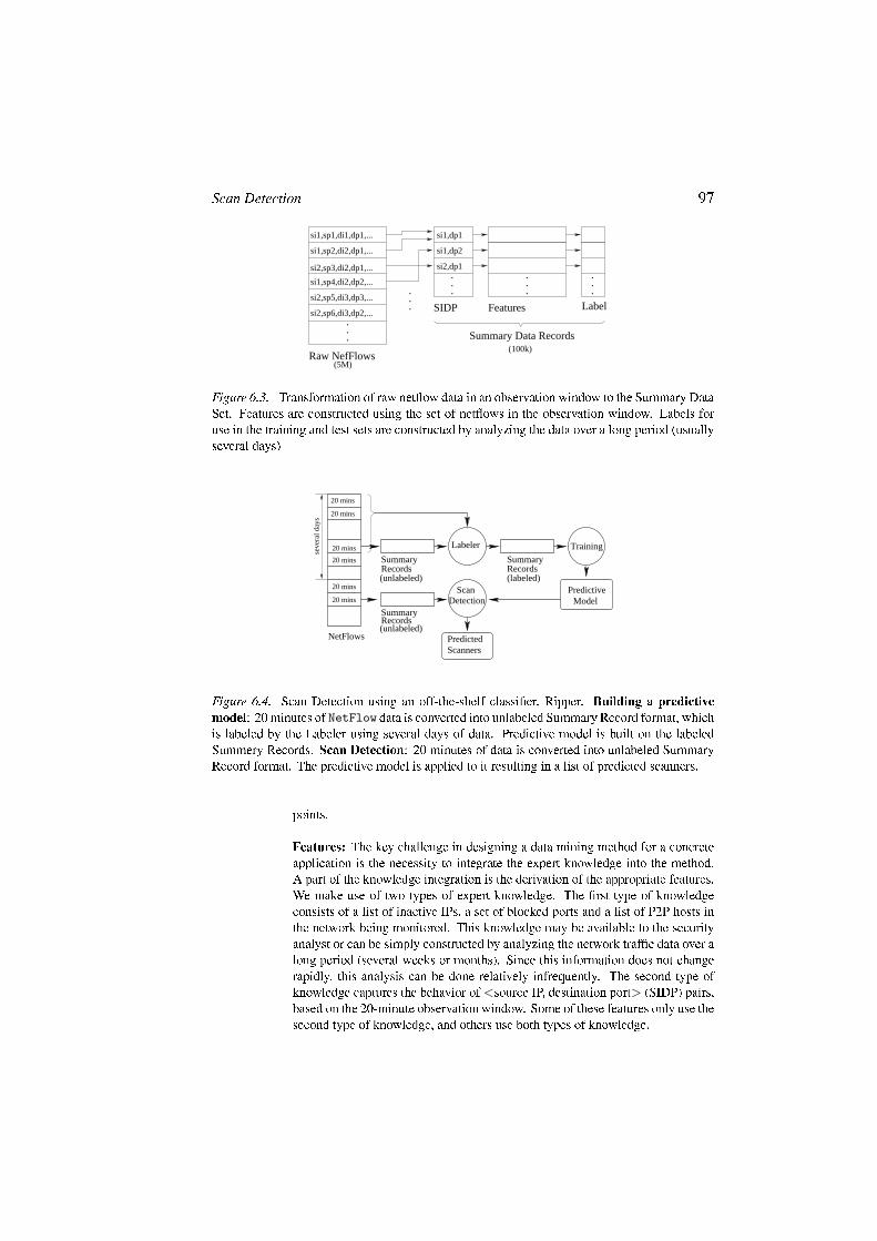
Methodology. Currently our solution is a batch-mode implementationthat analyzes data in windows of 20 minutes. For each 20-minute observationperiod, we transform the NetFlow data into a summary data set. Figure 6.3depicts this process. With our focus on incoming scans, each new summaryrecord corresponds to a potential scanner�that is pair of external source IPand destination port (SIDP). For each SIDP, the summary record contains a setof features constructed from the raw net�ows available during the observationwindow. Observation window size of 20 minutes is somewhat arbitrary. It needsto be large enough to generate features that have reliable values, but short enoughso that the construction of summary records does not take too much time ormemory.

Given a set of summary data records corresponding to an observation period,scan detection can be viewed as a classi�cation problem [24] in which each SIDP,whose source IP is external to the network being observed, is labeled as scannerif it was found scanning or non-scanner otherwise. This classi�cation problemcan be solved using predictive modeling techniques developed in the data miningand machine learning community if class labels (scanner/non-scanner) areavailable for a set of SIDPs that can be used as a training set.

Figure 6.4 depicts the overall paradigm. Each SIDP in the summary dataset for an observation period (typically 20 minutes) is labeled by analyzing thebehavior of the source IPs over a period of several days. Once a training setis constructed, a predictive model is built using Ripper. The Ripper generatedmodel can now be used on any summary data set to produce labels of SIDPs.

The success of this method depends on (1) whether we can label the dataaccurately and (2) whether we have derived the right set of features that facilitatethe extraction of knowledge. In the following sections, we will elaborate on these

Scan Detection 97

si1,sp1,di1,dp1,...

.

.

.

si1,sp4,di2,dp2,...

si2,sp3,di2,dp1,...

si1,sp2,di2,dp1,...

si2,sp5,di3,dp3,...

si2,sp6,di3,dp2,...

si2,dp1

si1,dp2

si1,dp1

.

.

.

.

.

.

.

.

.

SIDP Features Label

Raw NefFlows

Summary Data Records

.

.

.

(5M)

(100k)

Figure 6.3. Transformation of raw net�ow data in an observation window to the Summary DataSet. Features are constructed using the set of net�ows in the observation window. Labels foruse in the training and test sets are constructed by analyzing the data over a long period (usuallyseveral days)

ModelPredictive

Labeler

PredictedScanners

NetFlows

20 mins

20 mins

20 mins

20 mins

20 mins

20 mins

SummaryRecords(unlabeled)

SummaryRecords(labeled)

SummaryRecords(unlabeled)

Training

DetectionScan

seve

ral d

ays

Figure 6.4. Scan Detection using an off-the-shelf classi�er, Ripper. Building a predictivemodel: 20 minutes of NetFlow data is converted into unlabeled Summary Record format, whichis labeled by the Labeler using several days of data. Predictive model is built on the labeledSummery Records. Scan Detection: 20 minutes of data is converted into unlabeled SummaryRecord format. The predictive model is applied to it resulting in a list of predicted scanners.

points.

Features: The key challenge in designing a data mining method for a concreteapplication is the necessity to integrate the expert knowledge into the method.A part of the knowledge integration is the derivation of the appropriate features.We make use of two types of expert knowledge. The �rst type of knowledgeconsists of a list of inactive IPs, a set of blocked ports and a list of P2P hosts inthe network being monitored. This knowledge may be available to the securityanalyst or can be simply constructed by analyzing the network traf�c data over along period (several weeks or months). Since this information does not changerapidly, this analysis can be done relatively infrequently. The second type ofknowledge captures the behavior of <source IP, destination port> (SIDP) pairs,based on the 20-minute observation window. Some of these features only use thesecond type of knowledge, and others use both types of knowledge.


Labeling the Data Set: The goal of labeling is to generate a data set that can beused as training data set for Ripper. Given a set of summarized records corre-sponding to 20-minutes of observation with unknown labels (unknown scanningstatuses), the goal is to determine the actual labels with very high con�dence.The problem of computing the labels is very similar to the problem of scan de-tection except that we have the �exibility to observe the behavior of an SIDPover a long period. This makes it possible to declare certain SIDPs as scanneror non-scanner with great con�dence in many cases. For example, if a sourceIP s ip makes a few failed connection attempts on a speci�c port in a shorttime window, it may be hard to declare it a scanner. But if the behavior of s ipcan be observed over a long period of time (e.g. few days), it can be labeledas non-scanner (if it mostly makes successful connections on this port) orscanner (if most of its connection attempts are to destinations that never offeredservice on this port). However, there will situations, in which the above analysisdoes not offer any clear-cut evidence one way or the other. In such cases, welabel the SIDP as dontknow. For additional details on the labeling method, thereader is referred to [20].

Evaluation. For our experiments, we used real-world network trace datacollected at the University of Minnesota between the 1st and the 22nd March,2005. The University of Minnesota network consists of 5 class-B networks withmany autonomous subnetworks. Most of the IP space is allocated, but manysubnetworks have inactive IPs. We collected information about inactive IPsand P2P hosts over 22 days, and we used �ows in 20 minute windows during03/21/2005 (Mon.) and 03/22/2005 (Tue.) for constructing summary records forthe experiments. We took samples of 20-minute duration every 3 hours startingat midnight on March 21. A model was built for each of the 13 periods and testedon the remaining 12 periods. This allowed us to reduce possible dependence ona certain time of the day, and performed our experiments on each sample.

Table 6.7 describes the traf�c in terms of number of <source IP, destinationport> (SIDP) combinations pertaining to scanning-, P2P-, normal- and backscat-ter traf�c.

In our experimental evaluation, we provide comparison to TRW [11], as itis one of the state-of-the-art schemes. With the purpose of applying TRW forscanning worm containment, Weaver et al. [25] proposed a number of simpli�-cations so that TRW can be implemented in hardware. One of the simpli�cationsthey applied�without signi�cant loss of quality�is to perform the sequentialhypothesis testing in logarithmic space. TRW then can be modeled as count-ing: a counter is assigned to each source IP and this counter is incrementedupon a failed connection attempt and decremented upon a successful connectionestablishment.

Our implementation of TRW used in this paper for comparative evaluationdraws from the above ideas. If the count exceeds a certain positive threshold,we declare the source to be scanner, and if the counter falls below a negativethreshold, we declare the source to be normal.

The performance of a classi�er is measured in terms of precision, recall andF-measure. For a contingency table of

Scan Detection 99

Table 6.7. The distribution of (source IP, destination ports) (SIDPs) over the various traf�c typesfor each traf�c sample produced by our labeling method

ID Day.Time Total scan p2p normal backscatter dont-know01 0321.0000 67522 3984 28911 6971 4431 2322502 0321.0300 53333 5112 19442 9190 1544 1804503 0321.0600 56242 5263 19485 8357 2521 2061604 0321.0900 78713 5126 32573 10590 5115 2530905 0321.1200 93557 4473 38980 12354 4053 3369706 0321.1500 85343 3884 36358 10191 5383 2952707 0321.1800 92284 4723 39738 10488 5876 3145908 0321.2100 82941 4273 39372 8816 1074 2940609 0322.0000 69894 4480 33077 5848 1371 2511810 0322.0300 63621 4953 26859 4885 4993 2193111 0322.0600 60703 5629 25436 4467 3241 2193012 0322.0900 78608 4968 33783 7520 4535 2780213 0322.1200 91741 4130 43473 6319 4187 33632

classi�ed as classi�ed asScanner not Scanner

actual Scanner TP FNactual not Scanner FP TN

precision =TP

TP + FP

recall =TP

TP + FN

F−measure =2 ∗ prec ∗ recall

prec + recall.

Less formally, precision measures the percentage of scanning (source IP, des-tination port)-pairs (SIDPs) among the SIDPs that got declared scanners; recallmeasures the percentage of the actual scanners that were discovered; F-measurebalances between precision and recall.

To obtain a high-level view of the performance of our scheme, we built amodel on the 0321.0000 data set (ID 1) and tested it on the remaining 12 datasets. Figure 6.5 depicts the performance of our proposed scheme and that ofTRW on the same data sets 4.

One can see that not only does our proposed scheme outperform TRW by awide margin, it is also more stable: the performance varies less from data set todata set (the boxes in Figure 6.5 appear much smaller).

Figure 6.6 shows the actual values of precision, recall and F-measure for thedifferent data sets. The performance in terms of F-measure is consistently above90% with very high precision, which is important, because high false alarm ratescan rapidly deteriorate the usability of a system. The only jitter occurs on dataset # 7 and it was caused by a single source IP that scanned a single destinationhost on 614(!) different destination ports meanwhile touching only 4 blockedports. This source IP got misclassi�ed as P2P, since touching many destination


Prec Rec F−m Prec Rec F−m0

0.2

0.4

0.6

0.8

1

Ripper TRW

Performance Comparison

Figure 6.5. Performance comparison between the proposed scheme and TRW. From left toright, the six box plots correspond to the precision, recall and F-measure of our proposed schemeand the precision, recall and F-measure of TRW. Each box plot has three lines corresponding(from top downwards) to the upper quartile, median and lower quartile of the performance valuesobtained over the 13 data sets. The whiskers depict the best and worst performance.

3 5 7 9 11 130

0.2

0.4

0.6

0.8

1

Test Set ID

Performance of Ripper

Precision

Recall

F−measure

Figure 6.6. The performance of the proposed scheme on the 13 data sets in terms of precision(topmost line), F-measure (middle line) and recall (bottom line). The model was built on dataset ID 1.

ports (on a number of IPs) is characteristic of P2P. This single misclassi�cationintroduced 614 false negatives (recall that we are classifying SIDPs not sourceIPs). The reason for the misclassi�cation is that there were no vertical scannersin the training set � the highest number of destination ports scanned by a singlesource IP was 8, and this source IP touched over 47 destination IPs making itprimarily a horizontal scanner.

6. ConclusionMINDS is a suite of data mining algorithms which can be used as a tool by net-

work analysts to defend the network against attacks and emerging cyber threats.The various components of MINDS such as the scan detector, anomaly detectorand the pro�ling module detect different types of attacks and intrusions on acomputer network. The scan detector aims at detecting scans which are the per-

Acknowledgements 101

cusors to any network attack. The anomaly detection algorithm is very effectivein detecting behavioral anomalies in the network traf�c which typically translateto malicious activities such as dos traf�c, worms, policy violations and insideabuse. The pro�ling module helps a network analyst to understand the charac-teristics of the network traf�c and detect any deviations from the normal pro�le.Our analysis shows that the intrusions detected by MINDS are complementary tothose of traditional signature based systems, such as SNORT, which implies thatthey both can be combined to increase overall attack coverage. MINDS has showngreat operational success in detecting network intrusions in two live deploymentsat the University of Minnesota and as a part of the Interrogator [15] architectureat the US Army Research Lab�s Center for Intrusion Monitoring and Protection(ARL-CIMP).

7. AcknowledgementsThis work is supported by ARDA grant AR/F30602-03-C-0243, NSF grants

IIS-0308264 and ACI-0325949, and the US Army High Performance ComputingResearch Center under contract DAAD19-01-2-0014. The research reportedin this article was performed in collaboration with Paul Dokas, Yongdae Kim,Aleksandar Lazarevic, Haiyang Liu, Mark Shaneck, Jaideep Srivastava, MichaelSteinbach, Pang-Ning Tan, and Zhi-li Zhang. Access to computing facilities wasprovided by the AHPCRC and the Minnesota Supercomputing Institute.

Notes1. www.cs.umn.edu/research/minds2. www.splintered.net/sw/�ow-tools3. Typically, for a large sized network such as the University of Minnesota, data for a

10 minute long window is analyzed together4. The authors of TRW recommend a threshold of 4. In our experiments, we found,

that TRW can achieve better performance (in terms of F-measure) when we set the thresholdto 2, this is the threshold that was used in Figure 6.5, too.

References[1] Rakesh Agrawal, Tomasz Imieliski, and Arun Swami. Mining association

rules between sets of items in large databases. In Proceedings of the 1993ACM SIGMOD international conference on Management of data, pages207�216. ACM Press, 1993.

[2] Daniel Barbara and Sushil Jajodia, editors. Applications of Data Miningin Computer Security. Kluwer Academic Publishers, Norwell, MA, USA,2002.

[3] Markus M. Breunig, Hans-Peter Kriegel, Raymond T. Ng, and J Sander.Lof: identifying density-based local outliers. In Proceedings of the 2000ACM SIGMOD international conference on Management of data, pages93�104. ACM Press, 2000.

[4] Varun Chandola and Vipin Kumar. Summarization � compressing data intoan informative representation. In Fifth IEEE International Conference on


Data Mining, pages 98�105, Houston, TX, November 2005.[5] William W. Cohen. Fast effective rule induction. In International Confer-

ence on Machine Learning (ICML), 1995.[6] Dorothy E. Denning. An intrusion-detection model. IEEE Trans. Softw.

Eng., 13(2):222�232, 1987.[7] Eric Eilertson, Levent Ert�oz, Vipin Kumar, and Kerry Long. Minds � a

new approach to the information security process. In 24th Army ScienceConference. US Army, 2004.

[8] Levent Ert�oz, Eric Eilertson, Aleksander Lazarevic, Pang-Ning Tan, VipinKumar, Jaideep Srivastava, and Paul Dokas. MINDS - Minnesota IntrusionDetection System. In Data Mining - Next Generation Challenges and FutureDirections. MIT Press, 2004.

[9] Levent Ertoz, Michael Steinbach, and Vipin Kumar. Finding clusters ofdifferent sizes, shapes, and densities in noisy, high dimensional data. InProceedings of 3rd SIAM International Conference on Data Mining, May2003.

[10] Anil K. Jain and Richard C. Dubes. Algorithms for Clustering Data.Prentice-Hall, Inc., 1988.

[11] Jaeyeon Jung, Vern Paxson, Arthur W. Berger, and Hari Balakrishnan. Fastportscan detection using sequential hypothesis testing. In IEEE Symposiumon Security and Privacy, 2004.

[12] Vipin Kumar, Jaideep Srivastava, and Aleksander Lazarevic, editors. Man-aging Cyber Threats�Issues, Approaches and Challenges. Springer Verlag,May 2005.

[13] Aleksandar Lazarevic, Levent Ert�oz, Vipin Kumar, Aysel Ozgur, andJaideep Srivastava. A comparative study of anomaly detection schemes innetwork intrusion detection. In SIAM Conference on Data Mining (SDM),2003.

[14] C. Lickie and R. Kotagiri. A probabilistic approach to detecting networkscans. In Eighth IEEE Network Operations and Management, 2002.

[15] Kerry Long. Catching the cyber-spy, arl's interrogator. In 24th ArmyScience Conference. US Army, 2004.

[16] V. Paxon. Bro: a system for detecting network intruders in real-time. InEighth IEEE Network Operators and Management Symposium (NOMS),2002.

[17] Phillip A. Porras and Alfonso Valdes. Live traf�c analysis of tcp/ip gate-ways. In NDSS, 1998.

[18] Seth Robertson, Eric V. Siegel, Matt Miller, and Salvatore J. Stolfo.Surveillance detection in high bandwidth environments. In DARPA DIS-CEX III Conference, 2003.

[19] Martin Roesch. Snort: Lightweight intrusion detection for networks. InLISA, pages 229�238, 1999.

Acknowledgements 103

[20] Gyorgy Simon, Hui Xiong, Eric Eilertson, and Vipin Kumar. Scan detec-tion: A data mining approach. Technical Report AHPCRC 038, Universityof Minnesota � Twin Cities, 2005.

[21] Gyorgy Simon, Hui Xiong, Eric Eilertson, and Vipin Kumar. Scan detec-tion: A data mining approach. In Proceedings of SIAM Conference on DataMining (SDM), 2006.

[22] Anoop Singhal and Sushil Jajodia. Data mining for intrusion detection.In Data Mining and Knowledge Discovery Handbook, pages 1225�1237.Springer, 2005.

[23] Stuart Staniford, James A. Hoagland, and Joseph M. McAlerney. Practicalautomated detection of stealthy portscans. Journal of Computer Security,10(1/2):105�136, 2002.

[24] Pang-Ning Tan, Michael Steinbach, and Vipin Kumar. Introduction toData Mining. Addison-Wesley, May 2005.

[25] Nicholas Weaver, Stuart Staniford, and Vern Paxson. Very fast contain-ment of scanning worms. In 13th USENIX Security Symposium, 2004.

chapter 6 minds: architecture & design

Documents