chapter 6 graph algorithms - uni-freiburg.deac.informatik.uni-freiburg.de/teaching/ws18_19/... ·...

Chapter 6

Graph Algorithms

Algorithm TheoryWS 2018/19

Fabian Kuhn

Algorithm Theory, WS 2018/19 Fabian Kuhn 2

Example: Flow Network

𝑠 𝑡

𝑢

𝑣

20

20

10

10

30


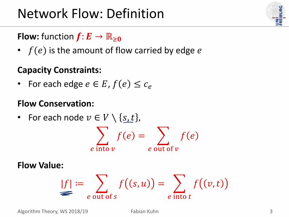
Network Flow: Definition

Flow: function 𝒇: 𝑬 → ℝ≥𝟎

• 𝑓(𝑒) is the amount of flow carried by edge 𝑒

Capacity Constraints:

• For each edge 𝑒 ∈ 𝐸, 𝑓 𝑒 ≤ 𝑐𝑒

Flow Conservation:

• For each node 𝑣 ∈ 𝑉 ∖ 𝑠, 𝑡 ,

𝑒 into 𝑣

𝑓 𝑒 =

𝑒 out of 𝑣

𝑓 𝑒

Flow Value:

|𝑓| ≔

𝑒 out of 𝑠

𝑓 𝑠, 𝑢 =

𝑒 into 𝑡

𝑓 𝑣, 𝑡


The Maximum-Flow Problem

Maximum Flow:

Given a flow network, find a flow of maximum possible value

• Classical graph optimization problem

• Many applications (also beyond the obvious ones)

• Requires new algorithmic techniques


Residual Graph

Given a flow network 𝐺 = 𝑉, 𝐸 with capacities 𝑐𝑒 (for 𝑒 ∈ 𝐸)

For a flow 𝑓 on 𝐺, define directed graph 𝐺𝑓 = (𝑉𝑓 , 𝐸𝑓) as follows:

• Node set 𝑉𝑓 = 𝑉

• For each edge 𝑒 = (𝑢, 𝑣) in 𝐸, there are two edges in 𝐸𝑓:

– forward edge 𝑒 = (𝑢, 𝑣) with residual capacity 𝑐𝑒 − 𝑓(𝑒)

– backward edge 𝑒′ = (𝑣, 𝑢) with residual capacity 𝑓(𝑒)

𝑠 𝑡

𝑢

𝑣

20

20

10

10

30

𝟐𝟎

𝟐𝟎

𝟐𝟎


Residual Graph: Example

𝑠

𝑥

𝑢

𝑦

𝑣

𝑤

𝑞

𝑧

𝑡

1520

20

15

10

10

20

15

20

15

15

15

10

5

20

20



Flow 𝒇

𝑠

𝑥

𝑢

𝑦

𝑣

𝑤

𝑞

𝑧

𝑡

1520

20

15

10

10

20

15

20

15

15

15

10

5

20

20𝟏𝟎

𝟓

𝟏𝟎

𝟓

𝟏𝟓

𝟓

𝟏𝟎

𝟏𝟎

𝟏𝟎

𝟐𝟎

𝟏𝟎

𝟏𝟎

𝟏𝟎

𝟏𝟎

510 15

5

0

15



Residual Graph 𝑮𝒇

𝑠

𝑥

𝑢

𝑦

𝑣

𝑤

𝑞

𝑧

𝑡

510 15

5

0

15

100

0 5

0

1015

15

0

10

10

05

20

10

10

10

1010 10

10

10

0

5 5

5


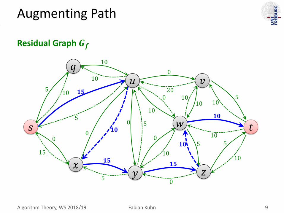
Augmenting Path

Residual Graph 𝑮𝒇

𝑠

𝑥

𝑢

𝑦

𝑣

𝑤

𝑞

𝑧

𝑡

510 𝟏𝟓

5

0

15

𝟏𝟎0

0 5

0

10𝟏𝟓

𝟏𝟓

0

10

10

05

20

𝟏𝟎

10

10

1010 10

10

𝟏𝟎

0

5 5

5


Augmenting Path

Augmenting Path

𝑠

𝑥

𝑢

𝑦

𝑣

𝑤

𝑞

𝑧

𝑡

1520

20

15

10

10

20

15

20

15

15

15

10

5

20

20𝟏𝟎

𝟓

𝟏𝟎

𝟓

𝟏𝟓

𝟓

𝟏𝟎

𝟏𝟎

𝟏𝟎

𝟐𝟎

𝟏𝟎

𝟏𝟎

𝟏𝟎

𝟏𝟎


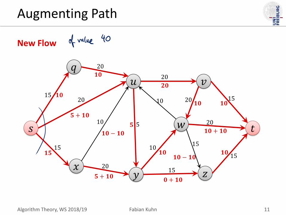
Augmenting Path

New Flow

𝑠

𝑥

𝑢

𝑦

𝑣

𝑤

𝑞

𝑧

𝑡

1520

20

15

10

10

20

15

20

15

15

15

10

5

20

20𝟏𝟎

𝟓 + 𝟏𝟎

𝟏𝟎 − 𝟏𝟎

𝟓 + 𝟏𝟎

𝟏𝟓

𝟓

𝟏𝟎

𝟏𝟎 + 𝟏𝟎

𝟏𝟎

𝟐𝟎

𝟏𝟎

𝟏𝟎 − 𝟏𝟎

𝟏𝟎

𝟏𝟎

𝟎 + 𝟏𝟎


Augmenting Path

Definition:An augmenting path 𝑃 is a (simple) 𝑠-𝑡-path on the residual graph 𝐺𝑓 on which each edge has residual capacity > 0.

bottleneck(𝑃, 𝑓): minimum residual capacity on any edge of theaugmenting path 𝑃

Augment flow 𝒇 to get flow 𝒇′:

• For every forward edge (𝑢, 𝑣) on 𝑃:

𝒇′ 𝒖, 𝒗 ≔ 𝒇 𝒖, 𝒗 + 𝐛𝐨𝐭𝐭𝐥𝐞𝐧𝐞𝐜𝐤 𝑷, 𝒇

• For every backward edge (𝑢, 𝑣) on 𝑃:

𝒇′ 𝒗, 𝒖 ≔ 𝒇 𝒗, 𝒖 − 𝐛𝐨𝐭𝐭𝐥𝐞𝐧𝐞𝐜𝐤(𝑷, 𝒇)


Augmented Flow

Lemma: Given a flow 𝑓 and an augmenting path 𝑃, the resulting augmented flow 𝑓′ is legal and its value is

𝒇′ = 𝒇 + 𝐛𝐨𝐭𝐭𝐥𝐞𝐧𝐞𝐜𝐤 𝑷, 𝒇 .

Proof:


Ford-Fulkerson Algorithm

• Improve flow using an augmenting path as long as possible:

1. Initially, 𝑓 𝑒 = 0 for all edges 𝑒 ∈ 𝐸, 𝐺𝑓 = 𝐺

2. while there is an augmenting 𝑠-𝑡-path 𝑃 in 𝐺𝑓 do

3. Let 𝑃 be an augmenting 𝑠-𝑡-path in 𝐺𝑓;

4. 𝑓′ ≔ augment(𝑓, 𝑃);

5. update 𝑓 to be 𝑓′;

6. update the residual graph 𝐺𝑓

7. end;


Ford-Fulkerson Running Time

Theorem: If all edge capacities are integers, the Ford-Fulkerson algorithm terminates after at most 𝐶 iterations, where

𝐶 = "max flow value" ≤

𝑒 out of 𝑠

𝑐𝑒 .

Proof:


Ford-Fulkerson Running Time

Theorem: If all edge capacities are integers, the Ford-Fulkerson algorithm can be implemented to run in 𝑂(𝑚𝐶) time.

Proof:


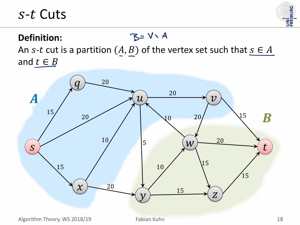
𝑠-𝑡 Cuts

Definition:An 𝑠-𝑡 cut is a partition (𝐴, 𝐵) of the vertex set such that 𝑠 ∈ 𝐴and 𝑡 ∈ 𝐵

𝑠

𝑥

𝑢

𝑦

𝑣

𝑤

𝑞

𝑧

𝑡

1520

20

15

10

10

20

15

20

15

15

15

10

5

20

20

𝑨

𝑩


Cut Capacity

Definition:The capacity 𝑐 𝐴, 𝐵 of an 𝑠-𝑡-cut (𝐴, 𝐵) is defined as

𝒄 𝑨,𝑩 ≔

𝒆 𝐨𝐮𝐭 𝐨𝐟 𝑨

𝒄𝒆 .

𝑠

𝑥

𝑢

𝑦

𝑣

𝑤

𝑞

𝑧

𝑡

1520

20

15

10

10

20

𝟏𝟓

20

15

15

15

10

𝟓

𝟐𝟎

𝟐𝟎

𝑨

𝑩


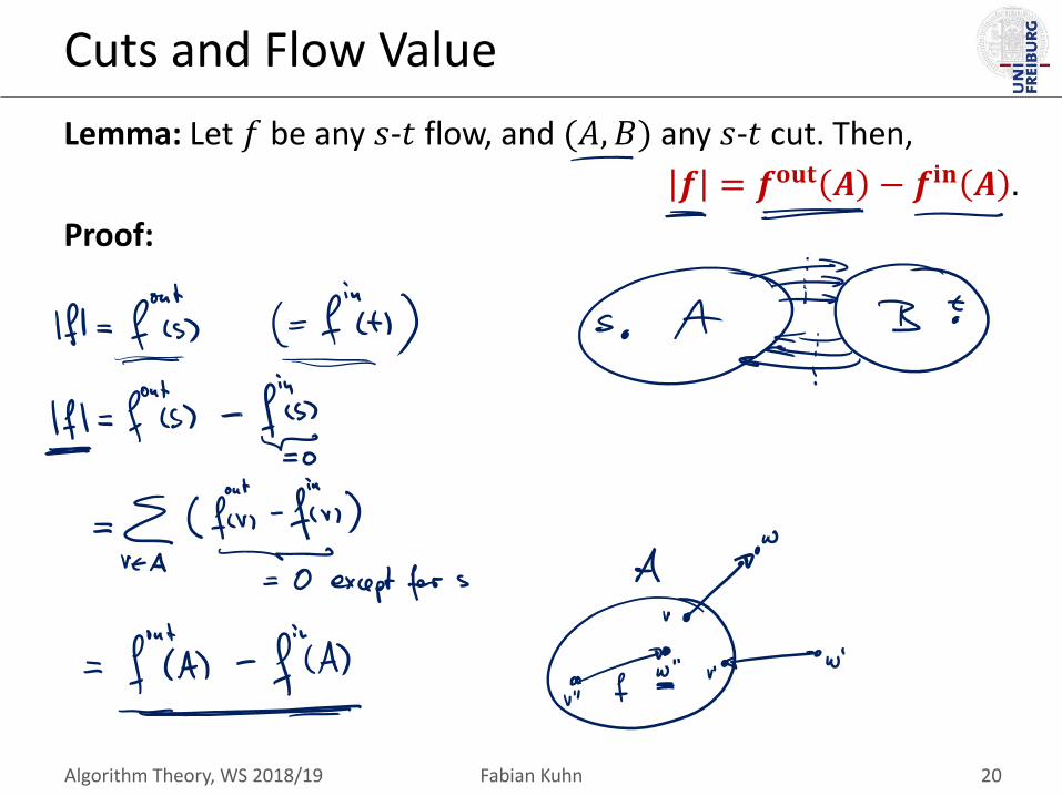
Cuts and Flow Value

Lemma: Let 𝑓 be any 𝑠-𝑡 flow, and (𝐴, 𝐵) any 𝑠-𝑡 cut. Then,

𝒇 = 𝒇𝐨𝐮𝐭 𝑨 − 𝒇𝐢𝐧 𝑨 .

Proof:


Cuts and Flow Value


𝒇 = 𝒇𝐨𝐮𝐭 𝑨 − 𝒇𝐢𝐧 𝑨 .


𝒇 = 𝒇𝐢𝐧 𝑩 − 𝒇𝐨𝐮𝐭 𝑩 .

Proof:


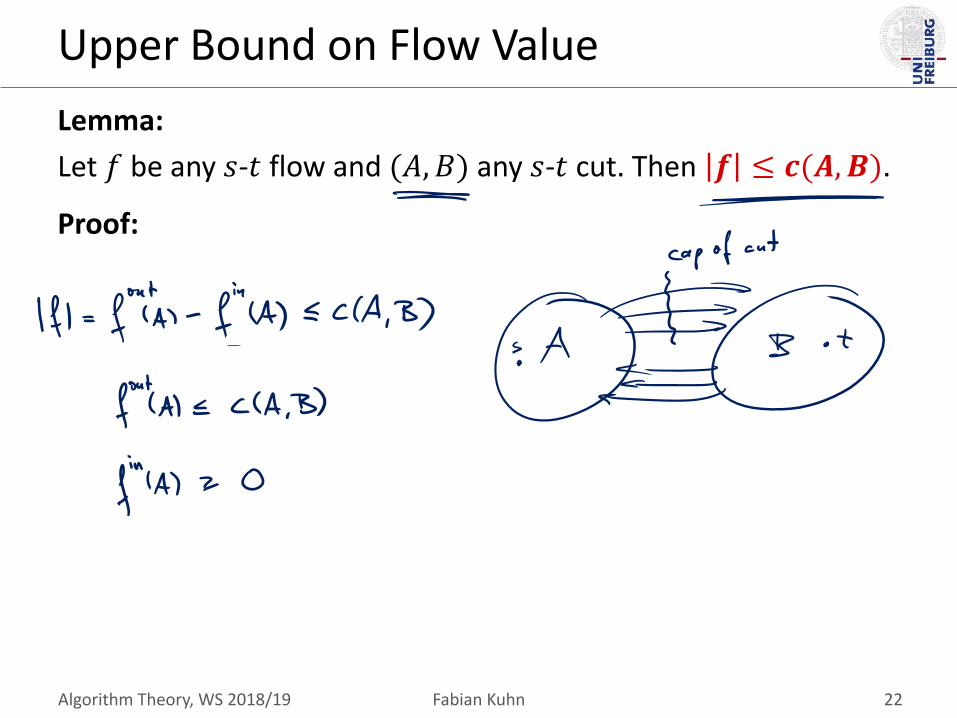
Upper Bound on Flow Value

Lemma:

Let 𝑓 be any 𝑠-𝑡 flow and (𝐴, 𝐵) any 𝑠-𝑡 cut. Then 𝒇 ≤ 𝒄(𝑨,𝑩).

Proof:


Ford-Fulkerson Gives Optimal Solution

Lemma: If 𝑓 is an 𝑠-𝑡 flow such that there is no augmenting path in 𝐺𝑓, then there is an 𝑠-𝑡 cut (𝐴∗, 𝐵∗) in 𝐺 for which

𝒇 = 𝒄 𝑨∗, 𝑩∗ .

Proof:

• Define 𝑨∗: set of nodes that can be reached from 𝑠 on a path with positive residual capacities in 𝐺𝑓:

• For 𝐵∗ = 𝑉 ∖ 𝐴∗, (𝐴∗, 𝐵∗) is an 𝑠-𝑡 cut– By definition 𝑠 ∈ 𝐴∗ and 𝑡 ∉ 𝐴∗




𝒇 = 𝒄 𝑨∗, 𝑩∗ .

Proof:



Theorem: The flow returned by the Ford-Fulkerson algorithm is a maximum flow.

Proof:


Min-Cut Algorithm

Ford-Fulkerson also gives a min-cut algorithm:

Theorem: Given a flow 𝑓 of maximum value, we can compute an 𝑠-𝑡 cut of minimum capacity in 𝑂(𝑚) time.

Proof:


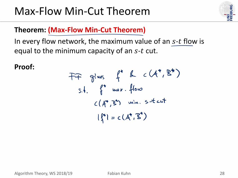
Max-Flow Min-Cut Theorem

Theorem: (Max-Flow Min-Cut Theorem)

In every flow network, the maximum value of an 𝑠-𝑡 flow is equal to the minimum capacity of an 𝑠-𝑡 cut.

Proof:


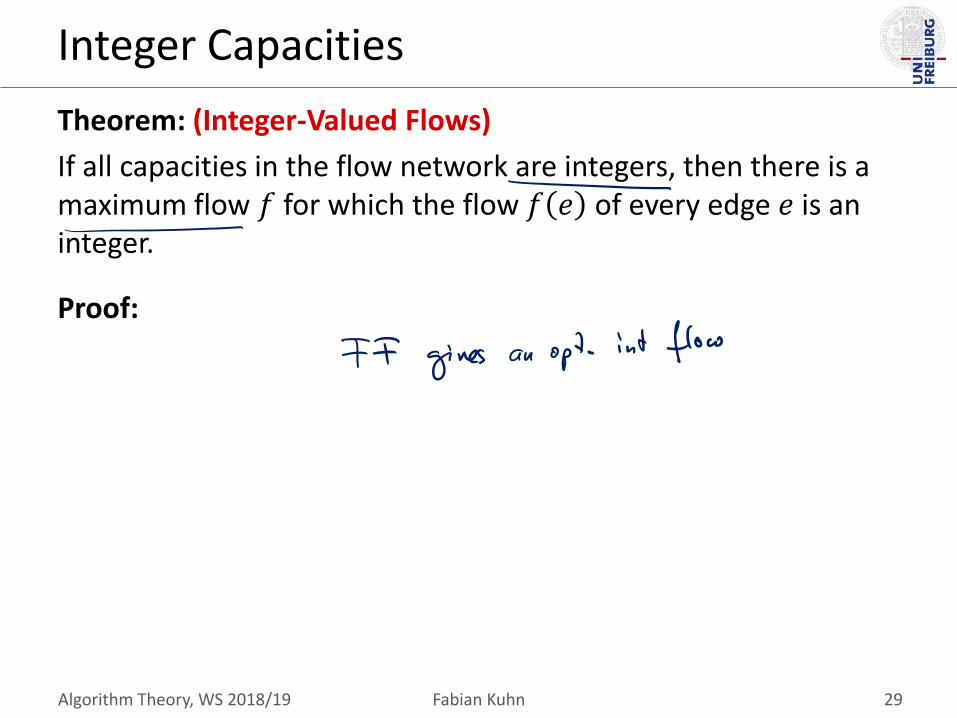
Integer Capacities

Theorem: (Integer-Valued Flows)

If all capacities in the flow network are integers, then there is a maximum flow 𝑓 for which the flow 𝑓 𝑒 of every edge 𝑒 is an integer.

Proof:


Non-Integer Capacities

What if capacities are not integers?

• rational capacities:– can be turned into integers by multiplying them with large enough integer

– algorithm still works correctly

• real (non-rational) capacities:– not clear whether the algorithm always terminates

• even for integer capacities, time can linearly depend on the value of the maximum flow


Slow Execution

• Number of iterations: 2000 (value of max. flow)

𝑠 𝑡

𝑢

𝑣

1000

1000

1000

1000

1

𝟏

𝟏

𝟏

𝟏

𝟏

𝟎

𝟐𝟐

𝟐 𝟐


Improved Algorithm

Idea: Find the best augmenting path in each step

• best: path 𝑃 with maximum bottleneck(𝑃, 𝑓)

• Best path might be rather expensive to find find almost best path

• Scaling parameter 𝚫: (initially, Δ = "max 𝑐𝑒 rounded down to next power of 2")

• As long as there is an augmenting path that improves the flow by at least Δ, augment using such a path

• If there is no such path: Δ ≔ ΤΔ 2


Scaling Parameter Analysis

Lemma: If all capacities are integers, number of different scaling parameters used is ≤ 1 + ⌊log2 𝐶⌋.

• 𝚫-scaling phase: Time during which scaling parameter is Δ


Length of a Scaling Phase

Lemma: If 𝑓 is the flow at the end of the Δ-scaling phase, the maximum flow in the network has value at most 𝑓 + 𝑚Δ.


Length of a Scaling Phase

Lemma: The number of augmentation in each scaling phase is at most 2𝑚.


Running Time: Scaling Max Flow Alg.

Theorem: The number of augmentations of the algorithm with scaling parameter and integer capacities is at most 𝑂(𝑚 log 𝐶). The algorithm can be implemented in time 𝑂 𝑚2 log 𝐶 .


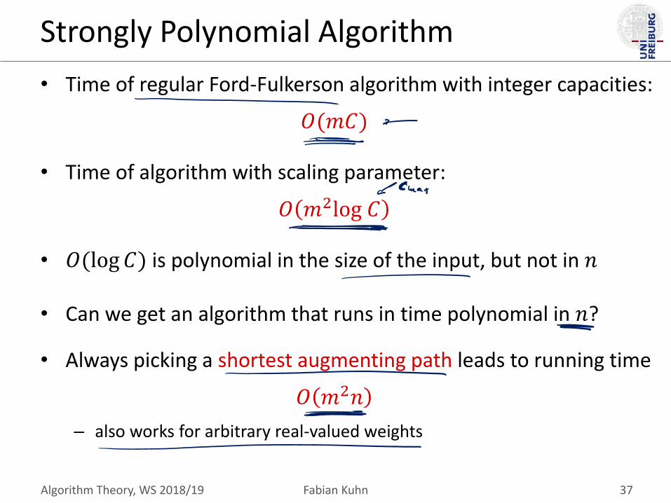
Strongly Polynomial Algorithm

• Time of regular Ford-Fulkerson algorithm with integer capacities:

𝑂(𝑚𝐶)

• Time of algorithm with scaling parameter:

𝑂 𝑚2log 𝐶

• 𝑂(log 𝐶) is polynomial in the size of the input, but not in 𝑛

• Can we get an algorithm that runs in time polynomial in 𝑛?

• Always picking a shortest augmenting path leads to running time

𝑂 𝑚2𝑛

– also works for arbitrary real-valued weights


Other Algorithms

• There are many other algorithms to solve the maximum flow problem, for example:

• Preflow-push algorithm:– Maintains a preflow (∀ nodes: inflow ≥ outflow)

– Alg. guarantees: As soon as we have a flow, it is optimal

– Detailed discussion in 2012/13 lecture

– Running time of basic algorithm: 𝑂 𝑚 ⋅ 𝑛2

– Doing steps in the “right” order: 𝑂 𝑛3

• Current best known complexity: 𝑶 𝒎 ⋅ 𝒏– For graphs with 𝑚 ≥ 𝑛1+𝜖 [King,Rao,Tarjan 1992/1994]

(for every constant 𝜖 > 0)

– For sparse graphs with 𝑚 ≤ 𝑛 Τ16 15−𝛿 [Orlin, 2013]

chapter 6 graph algorithms - uni-freiburg.deac.informatik.uni-freiburg.de/teaching/ws18_19/... ·...

Documents