chapter 6 examples: growth modeling and survival analysis - mplus
TRANSCRIPT

Examples: Growth, Survival, And N=1 Time Series Analysis
113
CHAPTER 6
EXAMPLES: GROWTH
MODELING, SURVIVAL
ANALYSIS, AND N=1 TIME
SERIES ANALYSIS
Growth models examine the development of individuals on one or more
outcome variables over time. These outcome variables can be observed
variables or continuous latent variables. Observed outcome variables
can be continuous, censored, binary, ordered categorical (ordinal),
counts, or combinations of these variable types if more than one growth
process is being modeled. In growth modeling, random effects are used
to capture individual differences in development. In a latent variable
modeling framework, the random effects are reconceptualized as
continuous latent variables, that is, growth factors.
Mplus takes a multivariate approach to growth modeling such that an
outcome variable measured at four occasions gives rise to a four-variate
outcome vector. In contrast, multilevel modeling typically takes a
univariate approach to growth modeling where an outcome variable
measured at four occasions gives rise to a single outcome for which
observations at the different occasions are nested within individuals,
resulting in two-level data. Due to the use of the multivariate approach,
Mplus does not consider a growth model to be a two-level model as in
multilevel modeling but a single-level model. With longitudinal data,
the number of levels in Mplus is one less than the number of levels in
conventional multilevel modeling. The multivariate approach allows
flexible modeling of the outcomes such as differences in residual
variances over time, correlated residuals over time, and regressions
among the outcomes over time.
In Mplus, there are two options for handling the relationship between the
outcome and time. One approach allows time scores to be parameters in
the model so that the growth function can be estimated. This is the
approach used in structural equation modeling. The second approach
allows time to be a variable that reflects individually-varying times of

CHAPTER 6
114
observations. This variable has a random slope. This is the approach
used in multilevel modeling. Random effects in the form of random
slopes are also used to represent individual variation in the influence of
time-varying covariates on outcomes.
Growth modeling in Mplus allows the analysis of multiple processes,
both parallel and sequential; regressions among growth factors and
random effects; growth modeling of factors measured by multiple
indicators; and growth modeling as part of a larger latent variable model.
Survival modeling in Mplus includes both discrete-time and continuous-
time analyses. Both types of analyses consider the time to an event.
Discrete-time survival analysis is used when the outcome is recorded
infrequently such as monthly or annually, typically leading to a limited
number of measurements. Continuous-time survival analysis is used
when the outcome is recorded more frequently such as hourly or daily,
typically leading to a large number of measurements. Survival modeling
is integrated into the general latent variable modeling framework so that
it can be part of a larger model.
N=1 time series analysis is used to analyze intensive longitudinal data
such as those obtained with ecological momentary assessments,
experience sampling methods, daily diary methods, and ambulatory
assessments for a single person. Such data typically have a large number
of time points, for example, twenty to two hundred. The measurements
are typically closely spaced in time. In Mplus, univariate autoregressive,
regression, cross-lagged, confirmatory factor analysis, Item Response
Theory, and structural equation models can be estimated for continuous,
binary, ordered categorical (ordinal), or combinations of these variable
types. Multilevel extensions of these models can be found in Chapter 9.
All growth and survival models can be estimated using the following
special features:
Single or multiple group analysis
Missing data
Complex survey data
Latent variable interactions and non-linear factor analysis using
maximum likelihood
Random slopes
Individually-varying times of observations

Examples: Growth, Survival, And N=1 Time Series Analysis
115
Linear and non-linear parameter constraints
Indirect effects including specific paths
Maximum likelihood estimation for all outcome types
Bootstrap standard errors and confidence intervals
Wald chi-square test of parameter equalities
For continuous, censored with weighted least squares estimation, binary,
and ordered categorical (ordinal) outcomes, multiple group analysis is
specified by using the GROUPING option of the VARIABLE command
for individual data or the NGROUPS option of the DATA command for
summary data. For censored with maximum likelihood estimation,
unordered categorical (nominal), and count outcomes, multiple group
analysis is specified using the KNOWNCLASS option of the
VARIABLE command in conjunction with the TYPE=MIXTURE
option of the ANALYSIS command. The default is to estimate the
model under missing data theory using all available data. The
LISTWISE option of the DATA command can be used to delete all
observations from the analysis that have missing values on one or more
of the analysis variables. Corrections to the standard errors and chi-
square test of model fit that take into account stratification, non-
independence of observations, and unequal probability of selection are
obtained by using the TYPE=COMPLEX option of the ANALYSIS
command in conjunction with the STRATIFICATION, CLUSTER, and
WEIGHT options of the VARIABLE command. The
SUBPOPULATION option is used to select observations for an analysis
when a subpopulation (domain) is analyzed. Latent variable interactions
are specified by using the | symbol of the MODEL command in
conjunction with the XWITH option of the MODEL command. Random
slopes are specified by using the | symbol of the MODEL command in
conjunction with the ON option of the MODEL command. Individually-
varying times of observations are specified by using the | symbol of the
MODEL command in conjunction with the AT option of the MODEL
command and the TSCORES option of the VARIABLE command.
Linear and non-linear parameter constraints are specified by using the
MODEL CONSTRAINT command. Indirect effects are specified by
using the MODEL INDIRECT command. Maximum likelihood
estimation is specified by using the ESTIMATOR option of the
ANALYSIS command. Bootstrap standard errors are obtained by using
the BOOTSTRAP option of the ANALYSIS command. Bootstrap
confidence intervals are obtained by using the BOOTSTRAP option of
the ANALYSIS command in conjunction with the CINTERVAL option

CHAPTER 6
116
of the OUTPUT command. The MODEL TEST command is used to test
linear restrictions on the parameters in the MODEL and MODEL
CONSTRAINT commands using the Wald chi-square test.
Graphical displays of observed data and analysis results can be obtained
using the PLOT command in conjunction with a post-processing
graphics module. The PLOT command provides histograms,
scatterplots, plots of individual observed and estimated values, and plots
of sample and estimated means and proportions/probabilities. These are
available for the total sample, by group, by class, and adjusted for
covariates. The PLOT command includes a display showing a set of
descriptive statistics for each variable. The graphical displays can be
edited and exported as a DIB, EMF, or JPEG file. In addition, the data
for each graphical display can be saved in an external file for use by
another graphics program.
Following is the set of growth modeling examples included in this
chapter:
6.1: Linear growth model for a continuous outcome
6.2: Linear growth model for a censored outcome using a censored
model*
6.3: Linear growth model for a censored outcome using a censored-
inflated model*
6.4: Linear growth model for a categorical outcome
6.5: Linear growth model for a categorical outcome using the Theta
parameterization
6.6: Linear growth model for a count outcome using a Poisson
model*
6.7: Linear growth model for a count outcome using a zero-inflated
Poisson model*
6.8: Growth model for a continuous outcome with estimated time
scores
6.9: Quadratic growth model for a continuous outcome
6.10: Linear growth model for a continuous outcome with time-
invariant and time-varying covariates
6.11: Piecewise growth model for a continuous outcome
6.12: Growth model with individually-varying times of observation
and a random slope for time-varying covariates for a continuous
outcome

Examples: Growth, Survival, And N=1 Time Series Analysis
117
6.13: Growth model for two parallel processes for continuous
outcomes with regressions among the random effects
6.14: Multiple indicator linear growth model for continuous
outcomes
6.15: Multiple indicator linear growth model for categorical
outcomes
6.16: Two-part (semicontinuous) growth model for a continuous
outcome*
6.17: Linear growth model for a continuous outcome with first-
order auto correlated residuals using non-linear constraints
6.18: Multiple group multiple cohort growth model
Following is the set of survival analysis examples included in this
chapter:
6.19: Discrete-time survival analysis
6.20: Continuous-time survival analysis using the Cox regression
model
6.21: Continuous-time survival analysis using a parametric
proportional hazards model
6.22: Continuous-time survival analysis using a parametric
proportional hazards model with a factor influencing survival*
Following is the set of N=1 time series analysis examples included in
this chapter:
6.23: N=1 time series analysis with a univariate first-order
autoregressive AR(1) model for a continuous dependent variable
6.24: N=1 time series analysis with a univariate first-order
autoregressive AR(1) model for a continuous dependent variable
with a covariate
6.25: N=1 time series analysis with a bivariate cross-lagged model
for continuous dependent variables
6.26: N=1 time series analysis with a first-order autoregressive
AR(1) confirmatory factor analysis (CFA) model with continuous
factor indicators
6.27: N=1 time series analysis with a first-order autoregressive
AR(1) IRT model with binary factor indicators
6.28: N=1 time series analysis with a bivariate cross-lagged model
with two factors and continuous factor indicators
CHAPTER 6
118
* Example uses numerical integration in the estimation of the model.
This can be computationally demanding depending on the size of the
problem.
EXAMPLE 6.1: LINEAR GROWTH MODEL FOR A
CONTINUOUS OUTCOME
TITLE: this is an example of a linear growth
model for a continuous outcome
DATA: FILE IS ex6.1.dat;
VARIABLE: NAMES ARE y11-y14 x1 x2 x31-x34;
USEVARIABLES ARE y11-y14;
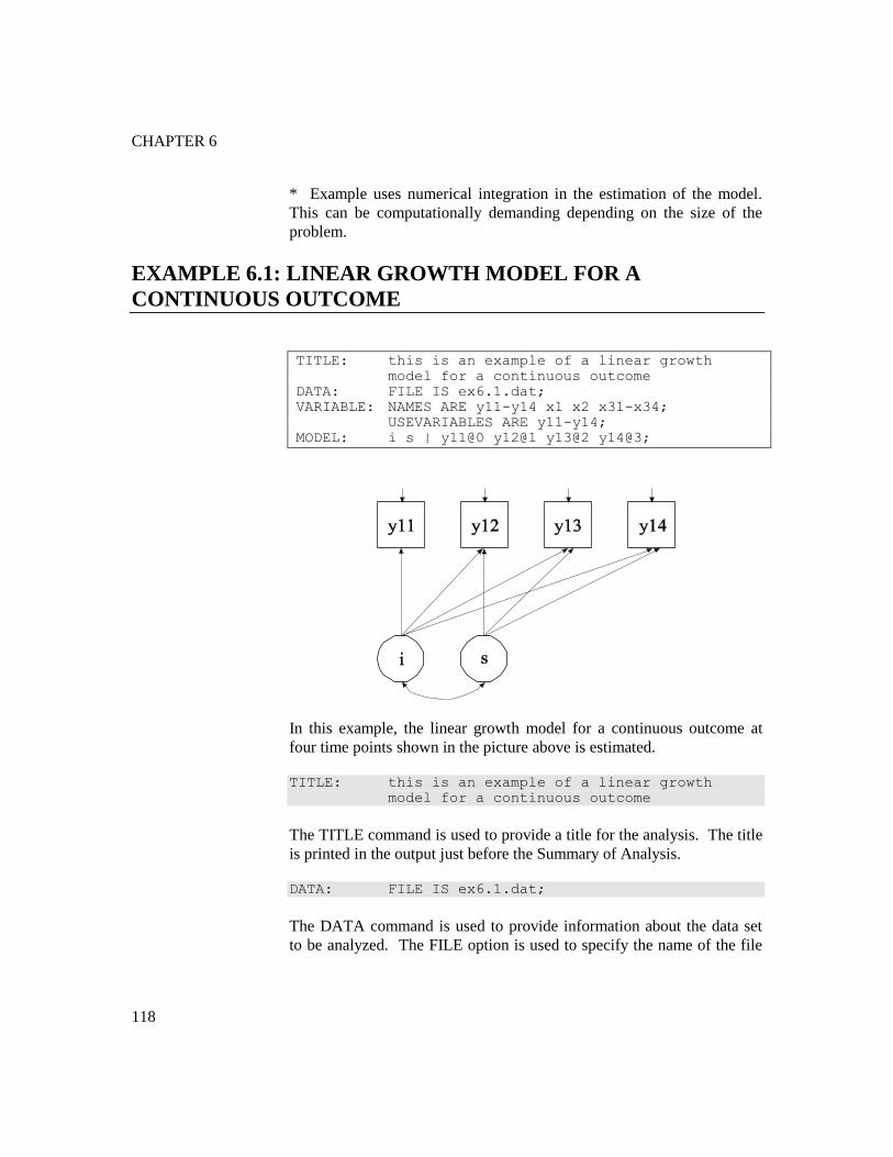
MODEL: i s | y11@0 y12@1 y13@2 y14@3;
In this example, the linear growth model for a continuous outcome at
four time points shown in the picture above is estimated.
TITLE: this is an example of a linear growth
model for a continuous outcome
The TITLE command is used to provide a title for the analysis. The title
is printed in the output just before the Summary of Analysis.
DATA: FILE IS ex6.1.dat;
The DATA command is used to provide information about the data set
to be analyzed. The FILE option is used to specify the name of the file

Examples: Growth, Survival, And N=1 Time Series Analysis
119
that contains the data to be analyzed, ex6.1.dat. Because the data set is
in free format, the default, a FORMAT statement is not required.
VARIABLE: NAMES ARE y11-y14 x1 x2 x31-x34;
USEVARIABLES ARE y11-y14;
The VARIABLE command is used to provide information about the
variables in the data set to be analyzed. The NAMES option is used to
assign names to the variables in the data set. The data set in this
example contains ten variables: y11, y12, y13, y14, x1, x2, x31, x32,
x33, and x34. Note that the hyphen can be used as a convenience feature
in order to generate a list of names. If not all of the variables in the data
set are used in the analysis, the USEVARIABLES option can be used to
select a subset of variables for analysis. Here the variables y11, y12,
y13, and y14 have been selected for analysis. They represent the
outcome measured at four equidistant occasions.
MODEL: i s | y11@0 y12@1 y13@2 y14@3;
The MODEL command is used to describe the model to be estimated.
The | symbol is used to name and define the intercept and slope factors
in a growth model. The names i and s on the left-hand side of the |
symbol are the names of the intercept and slope growth factors,
respectively. The statement on the right-hand side of the | symbol
specifies the outcome and the time scores for the growth model. The
time scores for the slope growth factor are fixed at 0, 1, 2, and 3 to
define a linear growth model with equidistant time points. The zero time
score for the slope growth factor at time point one defines the intercept
growth factor as an initial status factor. The coefficients of the intercept
growth factor are fixed at one as part of the growth model
parameterization. The residual variances of the outcome variables are
estimated and allowed to be different across time and the residuals are
not correlated as the default.
In the parameterization of the growth model shown here, the intercepts
of the outcome variables at the four time points are fixed at zero as the
default. The means and variances of the growth factors are estimated as
the default, and the growth factor covariance is estimated as the default
because the growth factors are independent (exogenous) variables. The
default estimator for this type of analysis is maximum likelihood. The
ESTIMATOR option of the ANALYSIS command can be used to select
a different estimator.

CHAPTER 6
120
EXAMPLE 6.2: LINEAR GROWTH MODEL FOR A
CENSORED OUTCOME USING A CENSORED MODEL
TITLE: this is an example of a linear growth
model for a censored outcome using a
censored model
DATA: FILE IS ex6.2.dat;
VARIABLE: NAMES ARE y11-y14 x1 x2 x31-x34;
USEVARIABLES ARE y11-y14;
CENSORED ARE y11-y14 (b);
ANALYSIS: ESTIMATOR = MLR;
MODEL: i s | y11@0 y12@1 y13@2 y14@3;
OUTPUT: TECH1 TECH8;
The difference between this example and Example 6.1 is that the
outcome variable is a censored variable instead of a continuous variable.
The CENSORED option is used to specify which dependent variables
are treated as censored variables in the model and its estimation, whether
they are censored from above or below, and whether a censored or
censored-inflated model will be estimated. In the example above, y11,
y12, y13, and y14 are censored variables. They represent the outcome
variable measured at four equidistant occasions. The b in parentheses
following y11-y14 indicates that y11, y12, y13, and y14 are censored
from below, that is, have floor effects, and that the model is a censored
regression model. The censoring limit is determined from the data. The
residual variances of the outcome variables are estimated and allowed to
be different across time and the residuals are not correlated as the
default.
The default estimator for this type of analysis is a robust weighted least
squares estimator. By specifying ESTIMATOR=MLR, maximum
likelihood estimation with robust standard errors using a numerical
integration algorithm is used. Note that numerical integration becomes
increasingly more computationally demanding as the number of factors
and the sample size increase. In this example, two dimensions of
integration are used with a total of 225 integration points. The
ESTIMATOR option of the ANALYSIS command can be used to select
a different estimator.
In the parameterization of the growth model shown here, the intercepts
of the outcome variables at the four time points are fixed at zero as the
Examples: Growth, Survival, And N=1 Time Series Analysis
121
default. The means and variances of the growth factors are estimated as
the default, and the growth factor covariance is estimated as the default
because the growth factors are independent (exogenous) variables. The
OUTPUT command is used to request additional output not included as
the default. The TECH1 option is used to request the arrays containing
parameter specifications and starting values for all free parameters in the
model. The TECH8 option is used to request that the optimization
history in estimating the model be printed in the output. TECH8 is
printed to the screen during the computations as the default. TECH8
screen printing is useful for determining how long the analysis takes. An
explanation of the other commands can be found in Example 6.1.
EXAMPLE 6.3: LINEAR GROWTH MODEL FOR A
CENSORED OUTCOME USING A CENSORED-INFLATED
MODEL
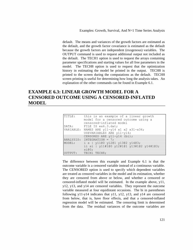
TITLE: this is an example of a linear growth
model for a censored outcome using a
censored-inflated model
DATA: FILE IS ex6.3.dat;
VARIABLE: NAMES ARE y11-y14 x1 x2 x31-x34;
USEVARIABLES ARE y11-y14;
CENSORED ARE y11-y14 (bi);
ANALYSIS: INTEGRATION = 7;
MODEL: i s | y11@0 y12@1 y13@2 y14@3;
ii si | y11#1@0 y12#1@1 y13#1@2 y14#1@3;
si@0;
OUTPUT: TECH1 TECH8;
The difference between this example and Example 6.1 is that the
outcome variable is a censored variable instead of a continuous variable.
The CENSORED option is used to specify which dependent variables
are treated as censored variables in the model and its estimation, whether
they are censored from above or below, and whether a censored or
censored-inflated model will be estimated. In the example above, y11,
y12, y13, and y14 are censored variables. They represent the outcome
variable measured at four equidistant occasions. The bi in parentheses
following y11-y14 indicates that y11, y12, y13, and y14 are censored
from below, that is, have floor effects, and that a censored-inflated
regression model will be estimated. The censoring limit is determined
from the data. The residual variances of the outcome variables are

CHAPTER 6
122
estimated and allowed to be different across time and the residuals are
not correlated as the default.
With a censored-inflated model, two growth models are estimated. The
first | statement describes the growth model for the continuous part of
the outcome for individuals who are able to assume values of the
censoring point and above. The residual variances of the outcome
variables are estimated and allowed to be different across time and the
residuals are not correlated as the default. The second | statement
describes the growth model for the inflation part of the outcome, the
probability of being unable to assume any value except the censoring
point. The binary latent inflation variable is referred to by adding to the
name of the censored variable the number sign (#) followed by the
number 1.
In the parameterization of the growth model for the continuous part of
the outcome, the intercepts of the outcome variables at the four time
points are fixed at zero as the default. The means and variances of the
growth factors are estimated as the default, and the growth factor
covariance is estimated as the default because the growth factors are
independent (exogenous) variables.
In the parameterization of the growth model for the inflation part of the
outcome, the intercepts of the outcome variable at the four time points
are held equal as the default. The mean of the intercept growth factor is
fixed at zero. The mean of the slope growth factor and the variances of
the intercept and slope growth factors are estimated as the default, and
the growth factor covariance is estimated as the default because the
growth factors are independent (exogenous) variables.
In this example, the variance of the slope growth factor si for the
inflation part of the outcome is fixed at zero. Because of this, the
covariances among si and all of the other growth factors are fixed at zero
as the default. The covariances among the remaining three growth
factors are estimated as the default.
The default estimator for this type of analysis is maximum likelihood
with robust standard errors using a numerical integration algorithm.
Note that numerical integration becomes increasingly more
computationally demanding as the number of factors and the sample size
increase. In this example, three dimensions of integration are used with
Examples: Growth, Survival, And N=1 Time Series Analysis
123
a total of 343 integration points. The INTEGRATION option of the
ANALYSIS command is used to change the number of integration points
per dimension from the default of 15 to 7. The ESTIMATOR option of
the ANALYSIS command can be used to select a different estimator.
The OUTPUT command is used to request additional output not
included as the default. The TECH1 option is used to request the arrays
containing parameter specifications and starting values for all free
parameters in the model. The TECH8 option is used to request that the
optimization history in estimating the model be printed in the output.
TECH8 is printed to the screen during the computations as the default.
TECH8 screen printing is useful for determining how long the analysis
takes. An explanation of the other commands can be found in Example
6.1.
EXAMPLE 6.4: LINEAR GROWTH MODEL FOR A
CATEGORICAL OUTCOME
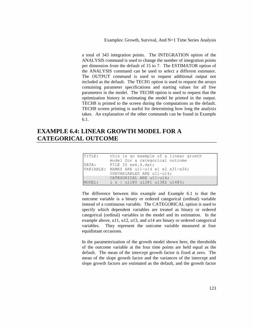
TITLE: this is an example of a linear growth
model for a categorical outcome
DATA: FILE IS ex6.4.dat;
VARIABLE: NAMES ARE u11-u14 x1 x2 x31-x34;
USEVARIABLES ARE u11-u14;
CATEGORICAL ARE u11-u14;
MODEL: i s | u11@0 u12@1 u13@2 u14@3;
The difference between this example and Example 6.1 is that the
outcome variable is a binary or ordered categorical (ordinal) variable
instead of a continuous variable. The CATEGORICAL option is used to
specify which dependent variables are treated as binary or ordered
categorical (ordinal) variables in the model and its estimation. In the
example above, u11, u12, u13, and u14 are binary or ordered categorical
variables. They represent the outcome variable measured at four
equidistant occasions.
In the parameterization of the growth model shown here, the thresholds
of the outcome variable at the four time points are held equal as the
default. The mean of the intercept growth factor is fixed at zero. The
mean of the slope growth factor and the variances of the intercept and
slope growth factors are estimated as the default, and the growth factor

CHAPTER 6
124
covariance is estimated as the default because the growth factors are
independent (exogenous) variables.
The default estimator for this type of analysis is a robust weighted least
squares estimator. The ESTIMATOR option of the ANALYSIS
command can be used to select a different estimator. With the weighted
least squares estimator, the probit model and the default Delta
parameterization for categorical outcomes are used. The scale factor for
the latent response variable of the categorical outcome at the first time
point is fixed at one as the default, while the scale factors for the latent
response variables at the other time points are free to be estimated. If a
maximum likelihood estimator is used, the logistic model for categorical
outcomes with a numerical integration algorithm is used (Hedeker &
Gibbons, 1994). Note that numerical integration becomes increasingly
more computationally demanding as the number of factors and the
sample size increase. An explanation of the other commands can be
found in Example 6.1.
EXAMPLE 6.5: LINEAR GROWTH MODEL FOR A
CATEGORICAL OUTCOME USING THE THETA
PARAMETERIZATION
TITLE: this is an example of a linear growth
model for a categorical outcome using the
Theta parameterization
DATA: FILE IS ex6.5.dat;
VARIABLE: NAMES ARE u11-u14 x1 x2 x31-x34;
USEVARIABLES ARE u11-u14;
CATEGORICAL ARE u11-u14;
ANALYSIS: PARAMETERIZATION = THETA;
MODEL: i s | u11@0 u12@1 u13@2 u14@3;
The difference between this example and Example 6.4 is that the Theta
parameterization instead of the default Delta parameterization is used.
In the Delta parameterization, scale factors for the latent response
variables of the observed categorical outcomes are allowed to be
parameters in the model, but residual variances for the latent response
variables are not. In the Theta parameterization, residual variances for
latent response variables are allowed to be parameters in the model, but
scale factors are not. Because the Theta parameterization is used, the

Examples: Growth, Survival, And N=1 Time Series Analysis
125
residual variance for the latent response variable at the first time point is
fixed at one as the default, while the residual variances for the latent
response variables at the other time points are free to be estimated. An
explanation of the other commands can be found in Examples 6.1 and
6.4.
EXAMPLE 6.6: LINEAR GROWTH MODEL FOR A COUNT
OUTCOME USING A POISSON MODEL
TITLE: this is an example of a linear growth
model for a count outcome using a Poisson
model
DATA: FILE IS ex6.6.dat;
VARIABLE: NAMES ARE u11-u14 x1 x2 x31-x34;
USEVARIABLES ARE u11-u14;
COUNT ARE u11-u14;
MODEL: i s | u11@0 u12@1 u13@2 u14@3;
OUTPUT: TECH1 TECH8;
The difference between this example and Example 6.1 is that the
outcome variable is a count variable instead of a continuous variable.
The COUNT option is used to specify which dependent variables are
treated as count variables in the model and its estimation and whether a
Poisson or zero-inflated Poisson model will be estimated. In the
example above, u11, u12, u13, and u14 are count variables. They
represent the outcome variable measured at four equidistant occasions.
In the parameterization of the growth model shown here, the intercepts
of the outcome variables at the four time points are fixed at zero as the
default. The means and variances of the growth factors are estimated as
the default, and the growth factor covariance is estimated as the default
because the growth factors are independent (exogenous) variables. The
default estimator for this type of analysis is maximum likelihood with
robust standard errors using a numerical integration algorithm. Note that
numerical integration becomes increasingly more computationally
demanding as the number of factors and the sample size increase. In this
example, two dimensions of integration are used with a total of 225
integration points. The ESTIMATOR option of the ANALYSIS
command can be used to select a different estimator. The OUTPUT
command is used to request additional output not included as the default.
The TECH1 option is used to request the arrays containing parameter
CHAPTER 6
126
specifications and starting values for all free parameters in the model.
The TECH8 option is used to request that the optimization history in
estimating the model be printed in the output. TECH8 is printed to the
screen during the computations as the default. TECH8 screen printing is
useful for determining how long the analysis takes. An explanation of
the other commands can be found in Example 6.1.
EXAMPLE 6.7: LINEAR GROWTH MODEL FOR A COUNT
OUTCOME USING A ZERO-INFLATED POISSON MODEL
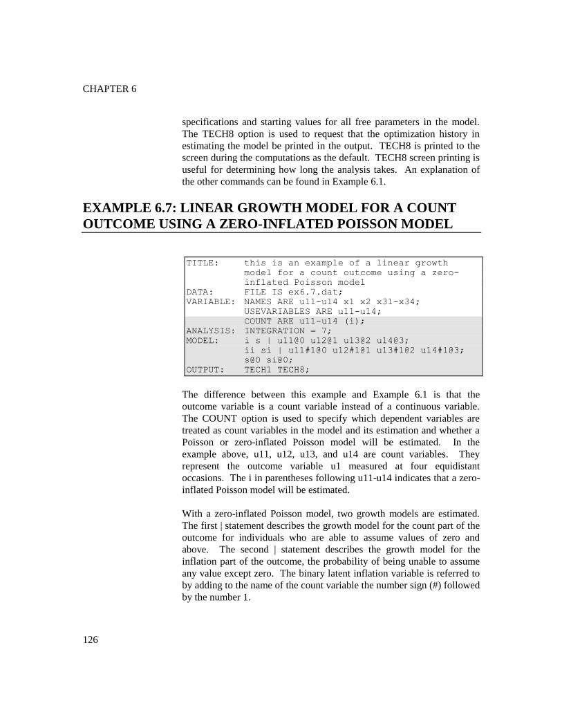
TITLE: this is an example of a linear growth
model for a count outcome using a zero-
inflated Poisson model
DATA: FILE IS ex6.7.dat;
VARIABLE: NAMES ARE u11-u14 x1 x2 x31-x34;
USEVARIABLES ARE u11-u14;
COUNT ARE u11-u14 (i);
ANALYSIS: INTEGRATION = 7;
MODEL: i s | u11@0 u12@1 u13@2 u14@3;
ii si | u11#1@0 u12#1@1 u13#1@2 u14#1@3;
s@0 si@0;
OUTPUT: TECH1 TECH8;
The difference between this example and Example 6.1 is that the
outcome variable is a count variable instead of a continuous variable.
The COUNT option is used to specify which dependent variables are
treated as count variables in the model and its estimation and whether a
Poisson or zero-inflated Poisson model will be estimated. In the
example above, u11, u12, u13, and u14 are count variables. They
represent the outcome variable u1 measured at four equidistant
occasions. The i in parentheses following u11-u14 indicates that a zero-
inflated Poisson model will be estimated.
With a zero-inflated Poisson model, two growth models are estimated.
The first | statement describes the growth model for the count part of the
outcome for individuals who are able to assume values of zero and
above. The second | statement describes the growth model for the
inflation part of the outcome, the probability of being unable to assume
any value except zero. The binary latent inflation variable is referred to
by adding to the name of the count variable the number sign (#) followed
by the number 1.

Examples: Growth, Survival, And N=1 Time Series Analysis
127
In the parameterization of the growth model for the count part of the
outcome, the intercepts of the outcome variables at the four time points
are fixed at zero as the default. The means and variances of the growth
factors are estimated as the default, and the growth factor covariance is
estimated as the default because the growth factors are independent
(exogenous) variables.
In the parameterization of the growth model for the inflation part of the
outcome, the intercepts of the outcome variable at the four time points
are held equal as the default. The mean of the intercept growth factor is
fixed at zero. The mean of the slope growth factor and the variances of
the intercept and slope growth factors are estimated as the default, and
the growth factor covariance is estimated as the default because the
growth factors are independent (exogenous) variables.
In this example, the variance of the slope growth factor s for the count
part and the slope growth factor si for the inflation part of the outcome
are fixed at zero. Because of this, the covariances among s, si, and the
other growth factors are fixed at zero as the default. The covariance
between the i and ii intercept growth factors is estimated as the default.
The default estimator for this type of analysis is maximum likelihood
with robust standard errors using a numerical integration algorithm.
Note that numerical integration becomes increasingly more
computationally demanding as the number of factors and the sample size
increase. In this example, two dimensions of integration are used with a
total of 49 integration points. The INTEGRATION option of the
ANALYSIS command is used to change the number of integration points
per dimension from the default of 15 to 7. The ESTIMATOR option of
the ANALYSIS command can be used to select a different estimator.
The OUTPUT command is used to request additional output not
included as the default. The TECH1 option is used to request the arrays
containing parameter specifications and starting values for all free
parameters in the model. The TECH8 option is used to request that the
optimization history in estimating the model be printed in the output.
TECH8 is printed to the screen during the computations as the default.
TECH8 screen printing is useful for determining how long the analysis
takes. An explanation of the other commands can be found in Example
6.1.

CHAPTER 6
128
EXAMPLE 6.8: GROWTH MODEL FOR A CONTINUOUS
OUTCOME WITH ESTIMATED TIME SCORES
TITLE: this is an example of a growth model for a
continuous outcome with estimated time
scores
DATA: FILE IS ex6.8.dat;
VARIABLE: NAMES ARE y11-y14 x1 x2 x31-x34;
USEVARIABLES ARE y11-y14;
MODEL: i s | y11@0 y12@1 y13*2 y14*3;
The difference between this example and Example 6.1 is that two of the
time scores are estimated. The | statement highlighted above shows how
to specify free time scores by using the asterisk (*) to designate a free
parameter. Starting values are specified as the value following the
asterisk (*). For purposes of model identification, two time scores must
be fixed for a growth model with two growth factors. In the example
above, the first two time scores are fixed at zero and one, respectively.
The third and fourth time scores are free to be estimated at starting
values of 2 and 3, respectively. The default estimator for this type of
analysis is maximum likelihood. The ESTIMATOR option of the
ANALYSIS command can be used to select a different estimator. An
explanation of the other commands can be found in Example 6.1.
EXAMPLE 6.9: QUADRATIC GROWTH MODEL FOR A
CONTINUOUS OUTCOME
TITLE: this is an example of a quadratic growth
model for a continuous outcome
DATA: FILE IS ex6.9.dat;
VARIABLE: NAMES ARE y11-y14 x1 x2 x31-x34;
USEVARIABLES ARE y11-y14;
MODEL: i s q | y11@0 y12@1 y13@2 y14@3;

Examples: Growth, Survival, And N=1 Time Series Analysis
129
The difference between this example and Example 6.1 is that the
quadratic growth model shown in the picture above is estimated. A
quadratic growth model requires three random effects: an intercept
factor (i), a linear slope factor (s), and a quadratic slope factor (q). The |
symbol is used to name and define the intercept and slope factors in the
growth model. The names i, s, and q on the left-hand side of the |
symbol are the names of the intercept, linear slope, and quadratic slope
factors, respectively. In the example above, the linear slope factor has
equidistant time scores of 0, 1, 2, and 3. The time scores for the
quadratic slope factor are the squared values of the linear time scores.
These time scores are automatically computed by the program.
In the parameterization of the growth model shown here, the intercepts
of the outcome variable at the four time points are fixed at zero as the
default. The means and variances of the three growth factors are
estimated as the default, and the three growth factors are correlated as
the default because they are independent (exogenous) variables. The
default estimator for this type of analysis is maximum likelihood. The
ESTIMATOR option of the ANALYSIS command can be used to select
a different estimator. An explanation of the other commands can be
found in Example 6.1.
CHAPTER 6
130
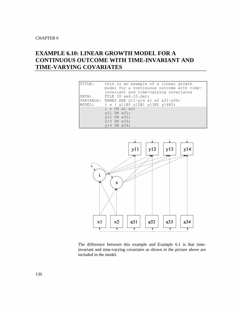
EXAMPLE 6.10: LINEAR GROWTH MODEL FOR A
CONTINUOUS OUTCOME WITH TIME-INVARIANT AND
TIME-VARYING COVARIATES
TITLE: this is an example of a linear growth
model for a continuous outcome with time-
invariant and time-varying covariates
DATA: FILE IS ex6.10.dat;
VARIABLE: NAMES ARE y11-y14 x1 x2 a31-a34;
MODEL: i s | y11@0 y12@1 y13@2 y14@3;
i s ON x1 x2;
y11 ON a31;
y12 ON a32;
y13 ON a33;
y14 ON a34;
The difference between this example and Example 6.1 is that time-
invariant and time-varying covariates as shown in the picture above are
included in the model.
Examples: Growth, Survival, And N=1 Time Series Analysis
131
The first ON statement describes the linear regressions of the two
growth factors on the time-invariant covariates x1 and x2. The next four
ON statements describe the linear regressions of the outcome variable on
the time-varying covariates a31, a32, a33, and a34 at each of the four
time points. The default estimator for this type of analysis is maximum
likelihood. The ESTIMATOR option of the ANALYSIS command can
be used to select a different estimator. An explanation of the other
commands can be found in Example 6.1.
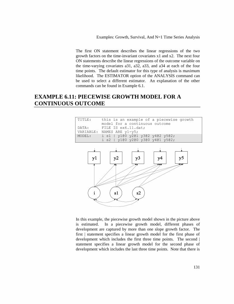
EXAMPLE 6.11: PIECEWISE GROWTH MODEL FOR A
CONTINUOUS OUTCOME
TITLE: this is an example of a piecewise growth
model for a continuous outcome
DATA: FILE IS ex6.11.dat;
VARIABLE: NAMES ARE y1-y5;
MODEL: i s1 | y1@0 y2@1 y3@2 y4@2 y5@2;
i s2 | y1@0 y2@0 y3@0 y4@1 y5@2;
In this example, the piecewise growth model shown in the picture above
is estimated. In a piecewise growth model, different phases of
development are captured by more than one slope growth factor. The
first | statement specifies a linear growth model for the first phase of
development which includes the first three time points. The second |
statement specifies a linear growth model for the second phase of
development which includes the last three time points. Note that there is

CHAPTER 6
132
one intercept growth factor i. It must be named in the specification of
both growth models when using the | symbol.
In the parameterization of the growth models shown here, the intercepts
of the outcome variable at the five time points are fixed at zero as the
default. The means and variances of the three growth factors are
estimated as the default, and the three growth factors are correlated as
the default because they are independent (exogenous) variables. The
default estimator for this type of analysis is maximum likelihood. The
ESTIMATOR option of the ANALYSIS command can be used to select
a different estimator. An explanation of the other commands can be
found in Example 6.1.
EXAMPLE 6.12: GROWTH MODEL WITH INDIVIDUALLY-
VARYING TIMES OF OBSERVATION AND A RANDOM
SLOPE FOR TIME-VARYING COVARIATES FOR A
CONTINUOUS OUTCOME
TITLE: this is an example of a growth model with
individually-varying times of observation
and a random slope for time-varying
covariates for a continuous outcome
DATA: FILE IS ex6.12.dat;
VARIABLE: NAMES ARE y1-y4 x a11-a14 a21-a24;
TSCORES = a11-a14;
ANALYSIS: TYPE = RANDOM;
MODEL: i s | y1-y4 AT a11-a14;
st | y1 ON a21;
st | y2 ON a22;
st | y3 ON a23;
st | y4 ON a24;
i s st ON x;
Examples: Growth, Survival, And N=1 Time Series Analysis
133
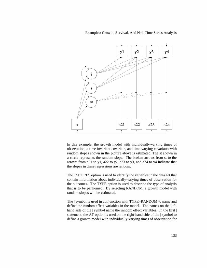
In this example, the growth model with individually-varying times of
observation, a time-invariant covariate, and time-varying covariates with
random slopes shown in the picture above is estimated. The st shown in
a circle represents the random slope. The broken arrows from st to the
arrows from a21 to y1, a22 to y2, a23 to y3, and a24 to y4 indicate that
the slopes in these regressions are random.
The TSCORES option is used to identify the variables in the data set that
contain information about individually-varying times of observation for
the outcomes. The TYPE option is used to describe the type of analysis
that is to be performed. By selecting RANDOM, a growth model with
random slopes will be estimated.
The | symbol is used in conjunction with TYPE=RANDOM to name and
define the random effect variables in the model. The names on the left-
hand side of the | symbol name the random effect variables. In the first |
statement, the AT option is used on the right-hand side of the | symbol to
define a growth model with individually-varying times of observation for

CHAPTER 6
134
the outcome variable. Two growth factors are used in the model, a
random intercept, i, and a random slope, s.
In the parameterization of the growth model shown here, the intercepts
of the outcome variables are fixed at zero as the default. The residual
variances of the outcome variables are free to be estimated as the
default. The residual covariances of the outcome variables are fixed at
zero as the default. The means, variances, and covariances of the
intercept and slope growth factors are free as the default.
The second, third, fourth, and fifth | statements use the ON option to
name and define the random slope variables in the model. The name on
the left-hand side of the | symbol names the random slope variable. The
statement on the right-hand side of the | symbol defines the random slope
variable. In the second | statement, the random slope st is defined by the
linear regression of the dependent variable y1 on the time-varying
covariate a21. In the third | statement, the random slope st is defined by
the linear regression of the dependent variable y2 on the time-varying
covariate a22. In the fourth | statement, the random slope st is defined
by the linear regression of the dependent variable y3 on the time-varying
covariate a23. In the fifth | statement, the random slope st is defined by
the linear regression of the dependent variable y4 on the time-varying
covariate a24. Random slopes with the same name are treated as one
variable during model estimation. The ON statement describes the linear
regressions of the intercept growth factor i, the slope growth factor s,
and the random slope st on the covariate x. The intercepts and residual
variances of, i, s, and st, are free as the default. The residual covariance
between i and s is estimated as the default. The residual covariances
between st and i and s are fixed at zero as the default. The default
estimator for this type of analysis is maximum likelihood with robust
standard errors. The estimator option of the ANALYSIS command can
be used to select a different estimator. An explanation of the other
commands can be found in Example 6.1.

Examples: Growth, Survival, And N=1 Time Series Analysis
135
EXAMPLE 6.13: GROWTH MODEL FOR TWO PARALLEL
PROCESSES FOR CONTINUOUS OUTCOMES WITH
REGRESSIONS AMONG THE RANDOM EFFECTS
TITLE: this is an example of a growth model for
two parallel processes for continuous
outcomes with regressions among the random
effects
DATA: FILE IS ex6.13.dat;
VARIABLE: NAMES ARE y11 y12 y13 y14 y21 y22 y23 y24;
MODEL: i1 s1 | y11@0 y12@1 y13@2 y14@3;
i2 s2 | y21@0 y22@1 y23@2 y24@3;
s1 ON i2;
s2 ON i1;

CHAPTER 6
136
In this example, the model for two parallel processes shown in the
picture above is estimated. Regressions among the growth factors are
included in the model.
The | statements are used to name and define the intercept and slope
growth factors for the two linear growth models. The names i1 and s1
on the left-hand side of the first | statement are the names of the intercept
and slope growth factors for the first linear growth model. The names i2
and s2 on the left-hand side of the second | statement are the names of
the intercept and slope growth factors for the second linear growth
model. The values on the right-hand side of the two | statements are the
time scores for the two slope growth factors. For both growth models,
the time scores of the slope growth factors are fixed at 0, 1, 2, and 3 to
define a linear growth model with equidistant time points. The zero time
score for the slope growth factor at time point one defines the intercept
factors as initial status factors. The coefficients of the intercept growth
factors are fixed at one as part of the growth model parameterization.
The residual variances of the outcome variables are estimated and
allowed to be different across time, and the residuals are not correlated
as the default.
In the parameterization of the growth model shown here, the intercepts
of the outcome variables at the four time points are fixed at zero as the
default. The means and variances of the intercept growth factors are
estimated as the default, and the intercept growth factor covariance is
estimated as the default because the intercept growth factors are
independent (exogenous) variables. The intercepts and residual
variances of the slope growth factors are estimated as the default, and
the slope growth factors are correlated as the default because residuals
are correlated for latent variables that do not influence any other variable
in the model except their own indicators.
The two ON statements describe the regressions of the slope growth
factor for each process on the intercept growth factor of the other
process. The default estimator for this type of analysis is maximum
likelihood. The ESTIMATOR option of the ANALYSIS command can
be used to select a different estimator. An explanation of the other
commands can be found in Example 6.1.
Examples: Growth, Survival, And N=1 Time Series Analysis
137
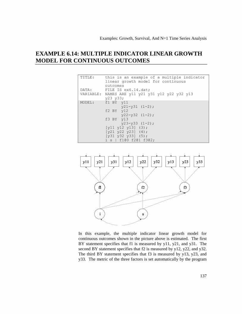
EXAMPLE 6.14: MULTIPLE INDICATOR LINEAR GROWTH
MODEL FOR CONTINUOUS OUTCOMES
TITLE: this is an example of a multiple indicator
linear growth model for continuous
outcomes
DATA: FILE IS ex6.14.dat;
VARIABLE: NAMES ARE y11 y21 y31 y12 y22 y32 y13
y23 y33;
MODEL: f1 BY y11
y21-y31 (1-2);
f2 BY y12
y22-y32 (1-2);
f3 BY y13
y23-y33 (1-2);
[y11 y12 y13] (3);
[y21 y22 y23] (4);
[y31 y32 y33] (5);
i s | f1@0 f2@1 f3@2;
In this example, the multiple indicator linear growth model for
continuous outcomes shown in the picture above is estimated. The first
BY statement specifies that f1 is measured by y11, y21, and y31. The
second BY statement specifies that f2 is measured by y12, y22, and y32.
The third BY statement specifies that f3 is measured by y13, y23, and
y33. The metric of the three factors is set automatically by the program

CHAPTER 6
138
by fixing the first factor loading in each BY statement to one. This
option can be overridden. The residual variances of the factor indicators
are estimated and the residuals are not correlated as the default.
A multiple indicator growth model requires measurement invariance of
the three factors across time. Measurement invariance is specified by
holding the intercepts and factor loadings of the factor indicators equal
over time. The (1-2) following the factor loadings in the three BY
statements uses the list function to assign equality labels to these
parameters. The label 1 is assigned to the factor loadings of y21, y22,
and y23 which holds these factor loadings equal across time. The label 2
is assigned to the factor loadings of y31, y32, and y33 which holds these
factor loadings equal across time. The factor loadings of y11, y21, and
y31 are fixed at one as described above. The bracket statements refer to
the intercepts. The (3) holds the intercepts of y11, y12, and y13 equal.
The (4) holds the intercepts of y21, y22, and y23 equal. The (5) holds
the intercepts of y31, y32, and y33 equal.
The | statement is used to name and define the intercept and slope factors
in the growth model. The names i and s on the left-hand side of the | are
the names of the intercept and slope growth factors, respectively. The
values on the right-hand side of the | are the time scores for the slope
growth factor. The time scores of the slope growth factor are fixed at 0,
1, and 2 to define a linear growth model with equidistant time points.
The zero time score for the slope growth factor at time point one defines
the intercept growth factor as an initial status factor. The coefficients of
the intercept growth factor are fixed at one as part of the growth model
parameterization. The residual variances of the factors f1, f2, and f3 are
estimated and allowed to be different across time, and the residuals are
not correlated as the default.
In the parameterization of the growth model shown here, the intercepts
of the factors f1, f2, and f3 are fixed at zero as the default. The mean of
the intercept growth factor is fixed at zero and the mean of the slope
growth factor is estimated as the default. The variances of the growth
factors are estimated as the default, and the growth factors are correlated
as the default because they are independent (exogenous) variables. The
default estimator for this type of analysis is maximum likelihood. The
ESTIMATOR option of the ANALYSIS command can be used to select
a different estimator. An explanation of the other commands can be
found in Example 6.1.

Examples: Growth, Survival, And N=1 Time Series Analysis
139
EXAMPLE 6.15: MULTIPLE INDICATOR LINEAR GROWTH
MODEL FOR CATEGORICAL OUTCOMES
TITLE: this is an example of a multiple indicator
linear growth model for categorical
outcomes
DATA: FILE IS ex6.15.dat;
VARIABLE: NAMES ARE u11 u21 u31 u12 u22 u32
u13 u23 u33;
CATEGORICAL ARE u11 u21 u31 u12 u22 u32
u13 u23 u33;
MODEL: f1 BY u11
u21-u31 (1-2);
f2 BY u12
u22-u32 (1-2);
f3 BY u13
u23-u33 (1-2);
[u11$1 u12$1 u13$1] (3);
[u21$1 u22$1 u23$1] (4);
[u31$1 u32$1 u33$1] (5);
{u11-u31@1 u12-u33};
i s | f1@0 f2@1 f3@2;
The difference between this example and Example 6.14 is that the factor
indicators are binary or ordered categorical (ordinal) variables instead of
continuous variables. The CATEGORICAL option is used to specify
which dependent variables are treated as binary or ordered categorical
(ordinal) variables in the model and its estimation. In the example
above, all of the factor indicators are categorical variables. The program
determines the number of categories for each indicator.
For binary and ordered categorical factor indicators, thresholds are
modeled rather than intercepts or means. The number of thresholds for a
categorical variable is equal to the number of categories minus one. In
the example above, the categorical variables are binary so they have one
threshold. Thresholds are referred to by adding to the variable name a $
followed by a number. The thresholds of the factor indicators are
referred to as u11$1, u12$1, u13$1, u21$1, u22$1, u23$1, u31$1, u32$1,
and u33$1. Thresholds are referred to in square brackets.
The growth model requires measurement invariance of the three factors
across time. Measurement invariance is specified by holding the
CHAPTER 6
140
thresholds and factor loadings of the factor indicators equal over time.
The (3) after the first bracket statement holds the thresholds of u11, u12,
and u13 equal. The (4) after the second bracket statement holds the
thresholds of u21, u22, and u23 equal. The (5) after the third bracket
statement holds the thresholds of u31, u32, and u33 equal. A list of
observed variables in curly brackets refers to scale factors. These are
part of the model with weighted least squares estimation and the Delta
parameterization. The scale factors for the latent response variables of
the categorical outcomes for the first factor are fixed at one, while the
scale factors for the latent response variables for the other factors are
free to be estimated. An explanation of the other commands can be
found in Examples 6.1 and 6.14.
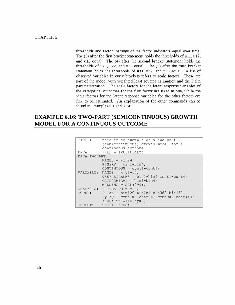
EXAMPLE 6.16: TWO-PART (SEMICONTINUOUS) GROWTH
MODEL FOR A CONTINUOUS OUTCOME
TITLE: this is an example of a two-part
(semicontinuous) growth model for a
continuous outcome
DATA: FILE = ex6.16.dat;
DATA TWOPART:
NAMES = y1-y4;
BINARY = bin1-bin4;
CONTINUOUS = cont1-cont4;
VARIABLE: NAMES = x y1-y4;
USEVARIABLES = bin1-bin4 cont1-cont4;
CATEGORICAL = bin1-bin4;
MISSING = ALL(999);
ANALYSIS: ESTIMATOR = MLR;
MODEL: iu su | bin1@0 bin2@1 bin3@2 bin4@3;
iy sy | cont1@0 cont2@1 cont3@2 cont4@3;
su@0; iu WITH sy@0;
OUTPUT: TECH1 TECH8;
Examples: Growth, Survival, And N=1 Time Series Analysis
141
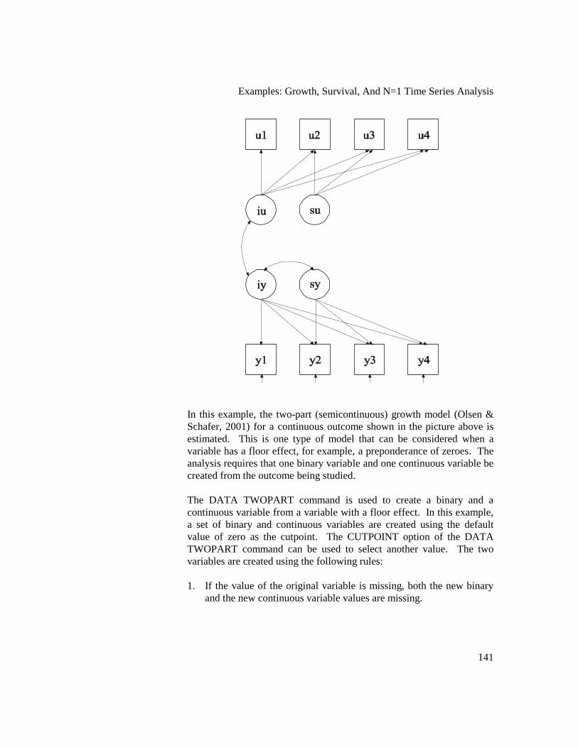
In this example, the two-part (semicontinuous) growth model (Olsen &
Schafer, 2001) for a continuous outcome shown in the picture above is
estimated. This is one type of model that can be considered when a
variable has a floor effect, for example, a preponderance of zeroes. The
analysis requires that one binary variable and one continuous variable be
created from the outcome being studied.
The DATA TWOPART command is used to create a binary and a
continuous variable from a variable with a floor effect. In this example,
a set of binary and continuous variables are created using the default
value of zero as the cutpoint. The CUTPOINT option of the DATA
TWOPART command can be used to select another value. The two
variables are created using the following rules:
1. If the value of the original variable is missing, both the new binary
and the new continuous variable values are missing.
CHAPTER 6
142
2. If the value of the original variable is greater than the cutpoint value,
the new binary variable value is one and the new continuous variable
value is the log of the original variable as the default.
3. If the value of the original variable is less than or equal to the
cutpoint value, the new binary variable value is zero and the new
continuous variable value is missing.
The TRANSFORM option of the DATA TWOPART command can be
used to select an alternative to the default log transformation of the new
continuous variables. One choice is no transformation.
The NAMES option of the DATA TWOPART command is used to
identify the variables from the NAMES option of the VARIABLE
command that are used to create a set of binary and continuous variables.
Variables y1, y2, y3, and y4 are used. The BINARY option is used to
assign names to the new set of binary variables. The names for the new
binary variables are bin1, bin2, bin3, and bin4. The CONTINUOUS
option is used to assign names to the new set of continuous variables.
The names for the new continuous variables are cont1, cont2, cont3, and
cont4. The new variables must be placed on the USEVARIABLES
statement of the VARIABLE command if they are used in the analysis.
The CATEGORICAL option is used to specify which dependent
variables are treated as binary or ordered categorical (ordinal) variables
in the model and its estimation. In the example above, bin1, bin2, bin3,
and bin4 are binary variables. The MISSING option is used to identify
the values or symbols in the analysis data set that are to be treated as
missing or invalid. In this example, the number 999 is the missing value
flag. The default is to estimate the model under missing data theory
using all available data. By specifying ESTIMATOR=MLR, a
maximum likelihood estimator with robust standard errors using a
numerical integration algorithm will be used. Note that numerical
integration becomes increasingly more computationally demanding as
the number of growth factors and the sample size increase. In this
example, one dimension of integration is used with a total of 15
integration points. The ESTIMATOR option of the ANALYSIS
command can be used to select a different estimator.
The first | statement specifies a linear growth model for the binary
outcome. The second | statement specifies a linear growth model for the
continuous outcome. In the parameterization of the growth model for

Examples: Growth, Survival, And N=1 Time Series Analysis
143
the binary outcome, the thresholds of the outcome variable at the four
time points are held equal as the default. The mean of the intercept
growth factor is fixed at zero. The mean of the slope growth factor and
the variances of the intercept and slope growth factors are estimated as
the default. In this example, the variance of the slope growth factor is
fized at zero for simplicity. In the parameterization of the growth model
for the continuous outcome, the intercepts of the outcome variables at
the four time points are fixed at zero as the default. The means and
variances of the growth factors are estimated as the default, and the
growth factors are correlated as the default because they are independent
(exogenous) variables.
It is often the case that not all growth factor covariances are significant
in two-part growth modeling. Fixing these at zero stabilizes the
estimation. This is why the growth factor covariance between iu and sy
is fixed at zero. The OUTPUT command is used to request additional
output not included as the default. The TECH1 option is used to request
the arrays containing parameter specifications and starting values for all
free parameters in the model. The TECH8 option is used to request that
the optimization history in estimating the model be printed in the output.
TECH8 is printed to the screen during the computations as the default.
TECH8 screen printing is useful for determining how long the analysis
takes. An explanation of the other commands can be found in Example
6.1.
CHAPTER 6
144
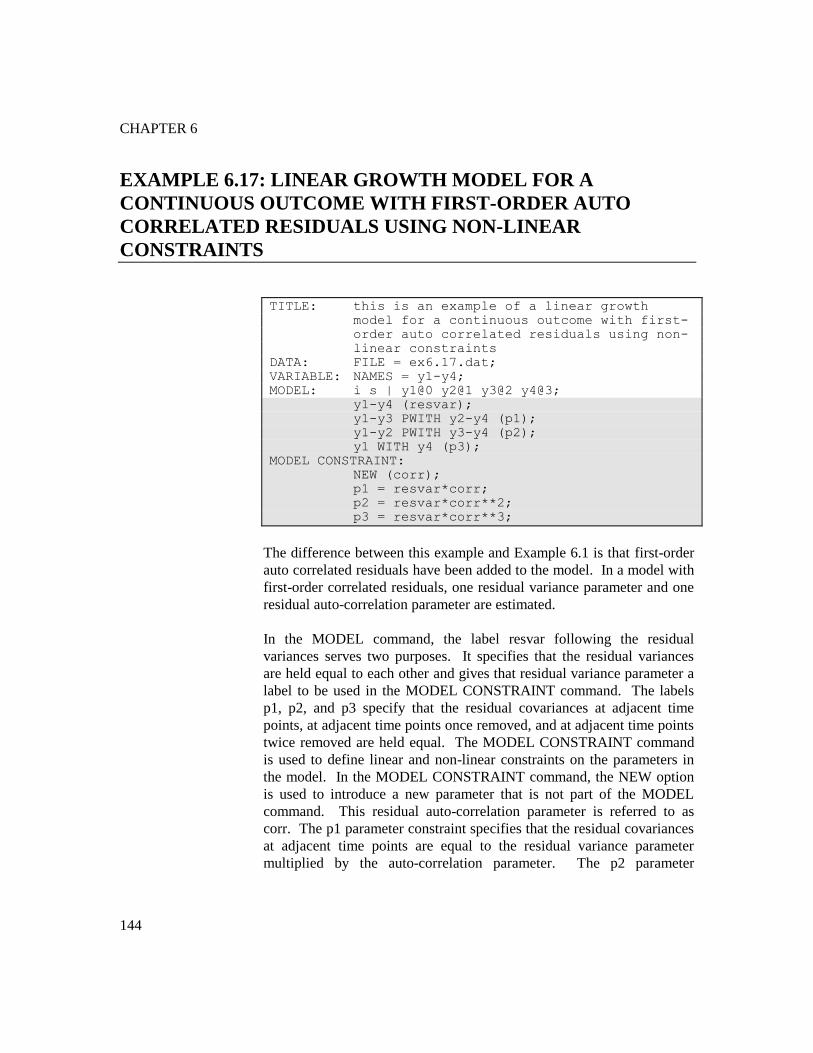
EXAMPLE 6.17: LINEAR GROWTH MODEL FOR A
CONTINUOUS OUTCOME WITH FIRST-ORDER AUTO
CORRELATED RESIDUALS USING NON-LINEAR
CONSTRAINTS
TITLE: this is an example of a linear growth
model for a continuous outcome with first-
order auto correlated residuals using non-
linear constraints
DATA: FILE = ex6.17.dat;
VARIABLE: NAMES = y1-y4;
MODEL: i s | y1@0 y2@1 y3@2 y4@3;
y1-y4 (resvar);
y1-y3 PWITH y2-y4 (p1);
y1-y2 PWITH y3-y4 (p2);
y1 WITH y4 (p3);
MODEL CONSTRAINT:
NEW (corr);
p1 = resvar*corr;
p2 = resvar*corr**2;
p3 = resvar*corr**3;
The difference between this example and Example 6.1 is that first-order
auto correlated residuals have been added to the model. In a model with
first-order correlated residuals, one residual variance parameter and one
residual auto-correlation parameter are estimated.
In the MODEL command, the label resvar following the residual
variances serves two purposes. It specifies that the residual variances
are held equal to each other and gives that residual variance parameter a
label to be used in the MODEL CONSTRAINT command. The labels
p1, p2, and p3 specify that the residual covariances at adjacent time
points, at adjacent time points once removed, and at adjacent time points
twice removed are held equal. The MODEL CONSTRAINT command
is used to define linear and non-linear constraints on the parameters in
the model. In the MODEL CONSTRAINT command, the NEW option
is used to introduce a new parameter that is not part of the MODEL
command. This residual auto-correlation parameter is referred to as
corr. The p1 parameter constraint specifies that the residual covariances
at adjacent time points are equal to the residual variance parameter
multiplied by the auto-correlation parameter. The p2 parameter

Examples: Growth, Survival, And N=1 Time Series Analysis
145
constraint specifies that the residual covariances at adjacent time points
once removed are equal to the residual variance parameter multiplied by
the auto-correlation parameter to the power of two. The p3 parameter
constraint specifies that the residual covariance at adjacent time points
twice removed is equal to the residual variance parameter multiplied by
the auto-correlation parameter to the power of three. An explanation of
the other commands can be found in Example 6.1.
EXAMPLE 6.18: MULTIPLE GROUP MULTIPLE COHORT
GROWTH MODEL
TITLE: this is an example of a multiple group
multiple cohort growth model
DATA: FILE = ex6.18.dat;
VARIABLE: NAMES = y1-y4 x a21-a24 g;
GROUPING = g (1 = 1990 2 = 1989 3 = 1988);
MODEL: i s |y1@0 [email protected] [email protected] [email protected];
[i] (1); [s] (2);
i (3); s (4);
i WITH s (5);
i ON x (6);
s ON x (7);
y1 ON a21;
y2 ON a22 (12);
y3 ON a23 (14);
y4 ON a24 (16);
y2-y4 (22-24);
MODEL 1989:
i s |[email protected] [email protected] [email protected] [email protected];
y1 ON a21;
y2 ON a22;
y3 ON a23;
y4 ON a24;
y1-y4;
MODEL 1988:
i s |[email protected] [email protected] [email protected] [email protected];
y1 ON a21 (12);
y2 ON a22 (14);
y3 ON a23 (16);
y4 ON a24;
y1-y3 (22-24);
y4;
OUTPUT: TECH1 MODINDICES(3.84);

CHAPTER 6
146
In this example, the multiple group multiple cohort growth model shown
in the picture above is estimated. Longitudinal research studies often
collect data on several different groups of individuals defined by their
birth year or cohort. This allows the study of development over a wider
age range than the length of the study and is referred to as an accelerated
or sequential cohort design. The interest in these studies is the
development of an outcome over age not measurement occasion. This
can be handled by rearranging the data so that age is the time axis using
the DATA COHORT command or using a multiple group approach as
described in this example. The advantage of the multiple group
approach is that it can be used to test assumptions of invariance of
growth parameters across cohorts.
In the multiple group approach the variables in the data set represent the
measurement occasions. In this example, there are four measurement
occasions: 2000, 2002, 2004, and 2006. Therefore there are four
variables to represent the outcome. In this example, there are three
cohorts with birth years 1988, 1989, and 1990. It is the combination of
the time of measurement and birth year that determines the ages
represented in the data. This is shown in the table below where rows
represent cohort and columns represent measurement occasion. The
Examples: Growth, Survival, And N=1 Time Series Analysis
147
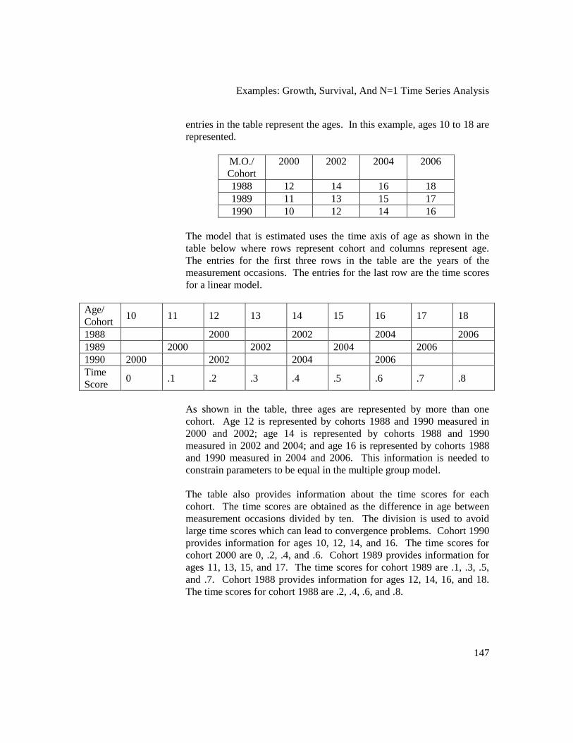
entries in the table represent the ages. In this example, ages 10 to 18 are
represented.
M.O./
Cohort
2000 2002 2004 2006
1988 12 14 16 18
1989 11 13 15 17
1990 10 12 14 16
The model that is estimated uses the time axis of age as shown in the
table below where rows represent cohort and columns represent age.
The entries for the first three rows in the table are the years of the
measurement occasions. The entries for the last row are the time scores
for a linear model.
Age/
Cohort 10 11 12 13 14 15 16 17 18
1988 2000 2002 2004 2006
1989 2000 2002 2004 2006
1990 2000 2002 2004 2006
Time
Score 0 .1 .2 .3 .4 .5 .6 .7 .8
As shown in the table, three ages are represented by more than one
cohort. Age 12 is represented by cohorts 1988 and 1990 measured in
2000 and 2002; age 14 is represented by cohorts 1988 and 1990
measured in 2002 and 2004; and age 16 is represented by cohorts 1988
and 1990 measured in 2004 and 2006. This information is needed to
constrain parameters to be equal in the multiple group model.
The table also provides information about the time scores for each
cohort. The time scores are obtained as the difference in age between
measurement occasions divided by ten. The division is used to avoid
large time scores which can lead to convergence problems. Cohort 1990
provides information for ages 10, 12, 14, and 16. The time scores for
cohort 2000 are 0, .2, .4, and .6. Cohort 1989 provides information for
ages 11, 13, 15, and 17. The time scores for cohort 1989 are .1, .3, .5,
and .7. Cohort 1988 provides information for ages 12, 14, 16, and 18.
The time scores for cohort 1988 are .2, .4, .6, and .8.

CHAPTER 6
148
The GROUPING option is used to identify the variable in the data set
that contains information on group membership when the data for all
groups are stored in a single data set. The information in parentheses
after the grouping variable name assigns labels to the values of the
grouping variable found in the data set. In the example above,
observations with g equal to 1 will be assigned the label 1990,
individuals with g equal to 2 will be assigned the label 1989, and
individuals with g equal to 3 will be assigned the label 1988. These
labels are used in conjunction with the MODEL command to specify
model statements specific to each group.
In multiple group analysis, two variations of the MODEL command are
used. They are MODEL and MODEL followed by a label. MODEL
describes the overall model to be estimated for each group. MODEL
followed by a label describes differences between the overall model and
the model for the group designated by the label. In the MODEL
command, the | symbol is used to name and define the intercept and
slope factors in a growth model. The names i and s on the left-hand side
of the | symbol are the names of the intercept and slope growth factors,
respectively. The statement on the right-hand side of the | symbol
specifies the outcome and the time scores for the growth model. The
time scores for the slope growth factor are fixed at 0, .2, .4, and .6.
These are the time scores for cohort 1990. The zero time score for the
slope growth factor at time point one defines the intercept growth factor
as an initial status factor for age 10. The coefficients of the intercept
growth factor are fixed at one as part of the growth model
parameterization. The residual variances of the outcome variables are
estimated and allowed to be different across age and the residuals are not
correlated as the default. The time scores for the other two cohorts are
specified in the group-specific MODEL commands. The group-specific
MODEL command for cohort 1989 fixes the time scores at .1, .3, .5, and
.7. The group-specific MODEL command for cohort 1988 fixes the time
scores at .2, .4, .6, and .8.
The equalities specified by the numbers in parentheses represent the
baseline assumption that the cohorts come from the same population.
Equalities specified in the overall MODEL command constrain
parameters to be equal across all groups. All parameters related to the
growth factors are constrained to be equal across all groups. Other
parameters are held equal when an age is represented by more than one
cohort. For example, the ON statement with the (12) equality in the

Examples: Growth, Survival, And N=1 Time Series Analysis
149
overall MODEL command describes the linear regression of y2 on the
time-varying covariate a22 for cohort 1990 at age 12. In the group-
specific MODEL command for cohort 1988, the ON statement with the
(12) equality describes the linear regression of y1 on the time-varying
covariate a21 for cohort 1988 at age 12. Other combinations of cohort
and age do not involve equality constraints. Cohort 1990 is the only
cohort that represents age 10; cohort 1989 is the only cohort that
represents ages 11, 13, 15, 17; and cohort 1988 is the only cohort that
represents age 18. Statements in the group-specific MODEL commands
relax equality constraints specified in the overall MODEL command.
An explanation of the other commands can be found in Example 6.1.
EXAMPLE 6.19: DISCRETE-TIME SURVIVAL ANALYSIS
TITLE: this is an example of a discrete-time
survival analysis
DATA: FILE IS ex6.19.dat;
VARIABLE: NAMES ARE u1-u4 x;
CATEGORICAL = u1-u4;
MISSING = ALL (999);
ANALYSIS: ESTIMATOR = MLR;
MODEL: f BY u1-u4@1;
f ON x;
f@0;
In this example, the discrete-time survival analysis model shown in the
picture above is estimated. Each u variable represents whether or not a
single non-repeatable event has occurred in a specific time period. The
value 1 means that the event has occurred, 0 means that the event has not

CHAPTER 6
150
occurred, and a missing value flag means that the event has occurred in a
preceding time period or that the individual has dropped out of the study
(Muthén & Masyn, 2005). The factor f is used to specify a proportional
odds assumption for the hazards of the event.
The MISSING option is used to identify the values or symbols in the
analysis data set that are to be treated as missing or invalid. In this
example, the number 999 is the missing value flag. The default is to
estimate the model under missing data theory using all available data.
The default estimator for this type of analysis is a robust weighted least
squares estimator. By specifying ESTIMATOR=MLR, maximum
likelihood estimation with robust standard errors is used. The BY
statement specifies that f is measured by u1, u2, u3, and u4 where the
factor loadings are fixed at one. This represents a proportional odds
assumption where the covariate x has the same influence on u1, u2, u3,
and u4. The ON statement describes the linear regression of f on the
covariate x. The residual variance of f is fixed at zero to correspond to a
conventional discrete-time survival model. An explanation of the other
commands can be found in Example 6.1.
EXAMPLE 6.20: CONTINUOUS-TIME SURVIVAL ANALYSIS
USING THE COX REGRESSION MODEL
TITLE: this is an example of a continuous-time
survival analysis using the Cox regression
model
DATA: FILE = ex6.20.dat;
VARIABLE: NAMES = t x tc;
SURVIVAL = t;
TIMECENSORED = tc (0 = NOT 1 = RIGHT);
MODEL: t ON x;
In this example, the continuous-time survival analysis model shown in
the picture above is estimated. This is the Cox regression model (Singer

Examples: Growth, Survival, And N=1 Time Series Analysis
151
& Willett, 2003). The profile likelihood method is used for model
estimation (Asparouhov et al., 2006).
The SURVIVAL option is used to identify the variables that contain
information about time to event and to provide information about the
number and lengths of the time intervals in the baseline hazard function
to be used in the analysis. The SURVIVAL option must be used in
conjunction with the TIMECENSORED option. In this example, t is the
variable that contains time-to-event information. Because nothing is
specified in parentheses behind t, the default baseline hazard function is
used. The TIMECENSORED option is used to identify the variables
that contain information about right censoring. In this example, the
variable is named tc. The information in parentheses specifies that the
value zero represents no censoring and the value one represents right
censoring. This is the default.
In the MODEL command, the ON statement describes the loglinear
regression of the time-to-event variable t on the covariate x. The default
estimator for this type of analysis is maximum likelihood with robust
standard errors. The estimator option of the ANALYSIS command can
be used to select a different estimator. An explanation of the other
commands can be found in Example 6.1.
EXAMPLE 6.21: CONTINUOUS-TIME SURVIVAL ANALYSIS
USING A PARAMETRIC PROPORTIONAL HAZARDS MODEL
TITLE: this is an example of a continuous-time
survival analysis using a parametric
proportional hazards model
DATA: FILE = ex6.21.dat;
VARIABLE: NAMES = t x tc;
SURVIVAL = t(20*1);
TIMECENSORED = tc (0 = NOT 1 = RIGHT);
ANALYSIS: BASEHAZARD = ON;
MODEL: [t#1-t#21];
t ON x;
The difference between this example and Example 6.20 is that a
parametric proportional hazards model is used instead of a Cox
regression model. In contrast to the Cox regression model, the

CHAPTER 6
152
parametric model estimates parameters and their standard errors for the
baseline hazard function (Asparouhov et al., 2006).
The SURVIVAL option is used to identify the variables that contain
information about time to event and to provide information about the
number and lengths of the time intervals in the baseline hazard function
to be used in the analysis. The SURVIVAL option must be used in
conjunction with the TIMECENSORED option. In this example, t is the
variable that contains time-to-event information. The numbers in
parentheses following the time-to-event variable specify that twenty time
intervals of length one are used in the analysis for the baseline hazard
function. The TIMECENSORED option is used to identify the variables
that contain information about right censoring. In this example, this
variable is named tc. The information in parentheses specifies that the
value zero represents no censoring and the value one represents right
censoring. This is the default.
The BASEHAZARD option of the ANALYSIS command is used with
continuous-time survival analysis to specify whether the baseline hazard
parameters are treated as model parameters or as auxiliary parameters.
The ON setting specifies that the parameters are treated as model
parameters. There are as many baseline hazard parameters as there are
time intervals plus one. These parameters can be referred to in the
MODEL command by adding to the name of the time-to-event variable
the number sign (#) followed by a number. In the MODEL command,
the bracket statement specifies that the 21 baseline hazard parameters are
part of the model.
The default estimator for this type of analysis is maximum likelihood
with robust standard errors. The estimator option of the ANALYSIS
command can be used to select a different estimator. An explanation of
the other commands can be found in Examples 6.1 and 6.20.

Examples: Growth, Survival, And N=1 Time Series Analysis
153
EXAMPLE 6.22: CONTINUOUS-TIME SURVIVAL ANALYSIS
USING A PARAMETRIC PROPORTIONAL HAZARDS MODEL
WITH A FACTOR INFLUENCING SURVIVAL
TITLE: this is an example of a continuous-time
survival analysis using a parametric
proportional hazards model with a factor
influencing survival
DATA: FILE = ex6.22.dat;
VARIABLE: NAMES = t u1-u4 x tc;
SURVIVAL = t (20*1);
TIMECENSORED = tc;
CATEGORICAL = u1-u4;
ANALYSIS: ALGORITHM = INTEGRATION;
BASEHAZARD = ON;
MODEL: f BY u1-u4;
[t#1-t#21];
t ON x f;
f ON x;
OUTPUT: TECH1 TECH8;
In this example, the continuous-time survival analysis model shown in
the picture above is estimated. The model is similar to Larsen (2005)

CHAPTER 6
154
although in this example the analysis uses a parametric baseline hazard
function (Asparouhov et al., 2006).
By specifying ALGORITHM=INTEGRATION, a maximum likelihood
estimator with robust standard errors using a numerical integration
algorithm will be used. Note that numerical integration becomes
increasingly more computationally demanding as the number of factors
and the sample size increase. In this example, one dimension of
integration is used with a total of 15 integration points. The
ESTIMATOR option of the ANALYSIS command can be used to select
a different estimator.
In the MODEL command the BY statement specifies that f is measured
by the binary indicators u1, u2, u3, and u4. The bracket statement
specifies that the 21 baseline hazard parameters are part of the model.
The first ON statement describes the loglinear regression of the time-to-
event variable t on the covariate x and the factor f. The second ON
statement describes the linear regression of f on the covariate x. An
explanation of the other commands can be found in Examples 6.1 and
6.21.
EXAMPLE 6.23: N=1 TIME SERIES ANALYSIS WITH A
UNIVARIATE FIRST-ORDER AUTOREGRESSIVE AR(1)
MODEL FOR A CONTINUOUS DEPENDENT VARIABLE
TITLE: this is an example of an N=1 time series
analysis with a univariate first-order
autoregressive AR(1) model for a
continuous dependent variable
DATA: FILE = ex6.23.dat;
VARIABLE: NAMES = y;
LAGGED = y(1);
ANALYSIS: ESTIMATOR = BAYES;
PROCESSORS = 2;
BITERATIONS = (2000);
MODEL: y ON y&1;
OUTPUT: TECH1 TECH8;
PLOT: TYPE = PLOT3;
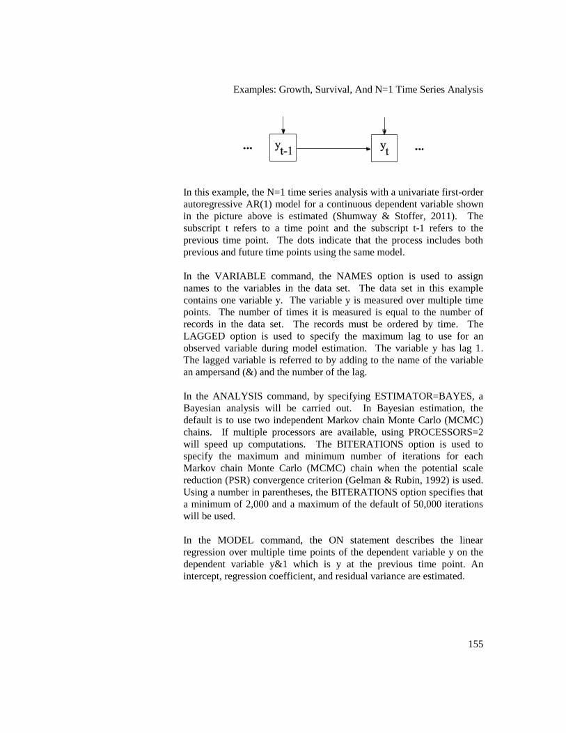
Examples: Growth, Survival, And N=1 Time Series Analysis
155
In this example, the N=1 time series analysis with a univariate first-order
autoregressive AR(1) model for a continuous dependent variable shown
in the picture above is estimated (Shumway & Stoffer, 2011). The
subscript t refers to a time point and the subscript t-1 refers to the
previous time point. The dots indicate that the process includes both
previous and future time points using the same model.
In the VARIABLE command, the NAMES option is used to assign
names to the variables in the data set. The data set in this example
contains one variable y. The variable y is measured over multiple time
points. The number of times it is measured is equal to the number of
records in the data set. The records must be ordered by time. The
LAGGED option is used to specify the maximum lag to use for an
observed variable during model estimation. The variable y has lag 1.
The lagged variable is referred to by adding to the name of the variable
an ampersand (&) and the number of the lag.
In the ANALYSIS command, by specifying ESTIMATOR=BAYES, a
Bayesian analysis will be carried out. In Bayesian estimation, the
default is to use two independent Markov chain Monte Carlo (MCMC)
chains. If multiple processors are available, using PROCESSORS=2
will speed up computations. The BITERATIONS option is used to
specify the maximum and minimum number of iterations for each
Markov chain Monte Carlo (MCMC) chain when the potential scale
reduction (PSR) convergence criterion (Gelman & Rubin, 1992) is used.
Using a number in parentheses, the BITERATIONS option specifies that
a minimum of 2,000 and a maximum of the default of 50,000 iterations
will be used.
In the MODEL command, the ON statement describes the linear
regression over multiple time points of the dependent variable y on the
dependent variable y&1 which is y at the previous time point. An
intercept, regression coefficient, and residual variance are estimated.
CHAPTER 6
156
An N=1 time series analysis with a univariate second-order
autoregressive AR(2) model can also be estimated. For this analysis, the
LAGGED option is specified as LAGGED = y (2); and the MODEL
command is specified as follows:
MODEL: y ON y&1 y&2;
In the MODEL command, the ON statement describes the linear
regression over multiple time points of the dependent variable y on the
dependent variable y&1 which is y at the previous time point and the
dependent variable y&2 which is y at two time points prior. An
intercept, two regression coefficients, and a residual variance are
estimated. A model where only y at lag 2 is used is specified as follows:
MODEL: y ON y&1@0 y&2;
where the coefficient for y at lag 1 is fixed at zero. An intercept,
regression coefficient, and residual variance are estimated.
The OUTPUT command is used to request additional output not
included as the default. The TECH1 option is used to request the arrays
containing parameter specifications and starting values for all free
parameters in the model. The TECH8 option is used to request that the
optimization history in estimating the model be printed in the output.
TECH8 is printed to the screen during the computations as the default.
TECH8 screen printing is useful for determining how long the analysis
takes and to check convergence using the PSR convergence criterion.
The PLOT command is used to request graphical displays of observed
data and analysis results. These graphical displays can be viewed after
the analysis is completed using a post-processing graphics module. The
trace plot and autocorrelation plot can be used to monitor the MCMC
iterations in terms of convergence and quality of the posterior
distribution for each parameter. The posterior distribution plot shows the
complete posterior distribution of the parameter estimate. Also available
are time series plots of observed values, autocorrelations at different
lags, and partial autocorrelations at different lags. An explanation of the
other commands can be found in Example 6.1.

Examples: Growth, Survival, And N=1 Time Series Analysis
157
EXAMPLE 6.24: N=1 TIME SERIES ANALYSIS WITH A
UNIVARIATE FIRST-ORDER AUTOREGRESSIVE AR(1)
MODEL FOR A CONTINUOUS DEPENDENT VARIABLE
WITH A COVARIATE
TITLE: this is an example of an N=1 time series
analysis with a univariate first-order
autoregressive AR(1) model for a
continuous dependent variable with a
covariate
DATA: FILE = ex6.24.dat;
VARIABLE: NAMES ARE y x;
LAGGED = y(1) x(1);
ANALYSIS: ESTIMATOR = BAYES;
PROCESSORS = 2;
BITERATIONS = (1000);
MODEL: y ON y&1 x x&1;
OUTPUT: TECH1 TECH8;
PLOT: TYPE = PLOT3;
In this example, the N=1 time series analysis with a univariate first-order
autoregressive AR(1) model for a continuous dependent variable with a
covariate shown in the picture above is estimated. The subscript t refers
to a time point and the subscript t-1 refers to the previous time point.
The dots indicate that the process includes both previous and future time
points using the same model.
In the MODEL command, the ON statement describes the linear
regression over multiple time points of the dependent variable y on the

CHAPTER 6
158
dependent variable y&1 which is y at the previous time point, a covariate
x, and a covariate x&1 which is x at the previous time point. An
intercept, three regression coefficients, and a residual variance are
estimated. An explanation of the other commands can be found in
Examples 6.1 and 6.23.
EXAMPLE 6.25: N=1 TIME SERIES ANALYSIS WITH A
BIVARIATE CROSS-LAGGED MODEL FOR CONTINUOUS
DEPENDENT VARIABLES
TITLE: this is an example of an N=1 time series
analysis with a bivariate cross-lagged
model for continuous dependent variables
DATA: FILE = ex6.25.dat;
VARIABLE: NAMES = y1 y2;
LAGGED = y1(1) y2(1);
ANALYSIS: ESTIMATOR = BAYES;
PROCESSORS = 2;
BITERATIONS = (500);
MODEL: y1 ON y1&1 y2&1;
y2 ON y2&1 y1&1;
OUTPUT: TECH1 TECH8;
PLOT: TYPE = PLOT3;
In this example, the N=1 time series analysis with a bivariate cross-
lagged model for continuous dependent variables shown in the picture
above is estimated. This model is also referred to as a first-order vector
autoregressive VAR(1) model, see e.g., Shumway and Stoffer (2011).
The subscript t refers to a time point and the subscript t-1 refers to the

Examples: Growth, Survival, And N=1 Time Series Analysis
159
previous time point. The dots indicate that the process includes both
previous and future time points using the same model.
In the MODEL command, the first ON statement describes the linear
regression over multiple time points of the dependent variable y1 on the
dependent variable y1&1 which is y1 at the previous time point, and the
dependent variable y2&1 which is y2 at the previous time point. The
second ON statement describes the linear regression over multiple time
points of the dependent variable y2 on the dependent variable y2&1
which is y2 at the previous time point, and the dependent variable y1&1
which is y1 at the previous time point. Two intercepts, four regression
coefficients, two residual variances, and one residual covariance are
estimated. An explanation of the other commands can be found in
Examples 6.1 and 6.23.
EXAMPLE 6.26: N=1 TIME SERIES ANALYSIS WITH A
FIRST-ORDER AUTOREGRESSIVE AR(1) CONFIRMATORY
FACTOR ANALYSIS (CFA) MODEL WITH CONTINUOUS
FACTOR INDICATORS
TITLE: this is an example of an N=1 time series
analysis with a first-order autoregressive
AR(1) confirmatory factor analysis (CFA)
model with continuous factor indicators
DATA: FILE = ex6.26.dat;
VARIABLE: NAMES = y1-y4;
ANALYSIS: ESTIMATOR = BAYES;
PROCESSORS = 2;
BITERATIONS = (2000);
MODEL: f BY y1-y4 (&1);
f ON f&1;
OUTPUT: TECH1 TECH8;
PLOT: TYPE = PLOT3;

CHAPTER 6
160
In this example, the N=1 time series analysis with a first-order
autoregressive AR(1) confirmatory factor analysis (CFA) model with
continuous factor indicators shown in the picture above is estimated.
This model is also referred to as a direct autoregressive factor score
(DAFS) model. For a discussion of N=1 time series factor analysis, also
referred to as dynamic factor analysis, see e.g., Molenaar (1985); Zhang,
Hamaker, and Nesselroade (2008); and Asparouhov, Hamaker, and
Muthén (2017). The subscript t refers to a time point and the subscript t-
1 refers to the previous time point. The dots indicate that the process
includes both previous and future time points using the same model.
In the MODEL command, the BY statement specifies that f is measured
by y1, y2, y3, and y4. The metric of the factor is set automatically by
the program by fixing the first factor loading to one. This option can be
overridden. An ampersand (&) followed by the number 1 is placed in
parentheses following the BY statement to indicate that the factor f at
lag 1 can be used in the analysis. The factor f at lag 1 is referred to as
f&1. The intercepts and residual variances of the factor indicators are
estimated and the residuals are not correlated as the default. The ON
statement describes the linear regression over multiple time points of the
factor f on the factor f&1 which is f at the previous time point. A
regression coefficient and residual variance of the factor are estimated.
The intercept of the factor is fixed at zero as the default.
A white noise factor score (WNFS) model (Zhang & Nesselroade, 2007)
can be estimated using the MODEL command below where instead of
regressing the factor f on f&1, the factor indicators y1, y2, y3, and y4 are
regressed on f&1.

Examples: Growth, Survival, And N=1 Time Series Analysis
161
MODEL: f BY y1-y4 (&1);
y1-y4 ON f&1;
An explanation of the other commands can be found in Examples 6.1
and 6.23.
EXAMPLE 6.27: N=1 TIME SERIES ANALYSIS WITH A
FIRST-ORDER AUTOREGRESSIVE AR(1) IRT MODEL WITH
BINARY FACTOR INDICATORS
TITLE: this is an example of an N=1 time series
analysis with a first-order autoregressive
AR(1) IRT model with binary factor
indicators
DATA: FILE = ex6.27.dat;
VARIABLE: NAMES = u1-u4;
CATEGORICAL = u1-u4;
ANALYSIS: ESTIMATOR = BAYES;
PROCESSORS = 2;
BITERATIONS = (2000);
MODEL: f BY u1-u4*(&1);
f@1;
f ON f&1;
OUTPUT: TECH1 TECH8;
PLOT: TYPE = PLOT3;
In this example, an N=1 time series analysis with a first-order
autoregressive AR(1) IRT model with binary factor indicators is
estimated. The subscript t refers to a time point and the subscript t-1
refers to the previous time point. The dots indicate that the process
includes both previous and future time points using the same model.
The CATEGORICAL option specifies that the variables u1, u2, u3, and
u4 are binary. In the MODEL command, the BY statement specifies that
f is measured by u1, u2, u3, and u4. The metric of the factor is set
automatically by the program by fixing the first factor loading to one.
The asterisk following u1-u4 overrides this default. The metric of the
factor is set by fixing the factor residual variance to one. An ampersand
(&) followed by the number 1 is placed in parentheses following the BY
statement to indicate that the factor f at lag 1 can be used in the analysis.
The factor f at lag 1 is referred to as f&1. The thresholds of the factor
indicators are estimated as the default. The ON statement describes the

CHAPTER 6
162
linear regression over multiple time points of the factor f on the factor
f&1 which is f at the previous time point. A regression coefficient and
residual variance of the factor are estimated. The intercept of the factor
is fixed at zero as the default. An explanation of the other commands
can be found in Examples 6.1, 6.4, and 6.23.
EXAMPLE 6.28: N=1 TIME SERIES ANALYSIS WITH A
BIVARIATE CROSS-LAGGED MODEL WITH TWO FACTORS
AND CONTINUOUS FACTOR INDICATORS
TITLE: this is an example of an N=1 time series
analysis with a bivariate cross-lagged
model with two factors and continuous
factor indicators
DATA: FILE = ex6.28.dat;
VARIABLE: NAMES = y11-y14 y21-y24;
ANALYSIS: ESTIMATOR = BAYES;
PROCESSORS = 2;
BITERATIONS = (2000);
MODEL: f1 BY y11-y14 (&1);
f2 BY y21-y24 (&1);
f1 ON f1&1 f2&1;
f2 ON f2&1 f1&1;
OUTPUT: TECH1 TECH8;
PLOT: TYPE = PLOT3;
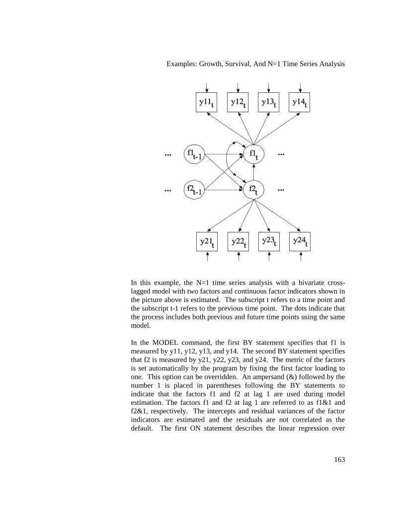
Examples: Growth, Survival, And N=1 Time Series Analysis
163
In this example, the N=1 time series analysis with a bivariate cross-
lagged model with two factors and continuous factor indicators shown in
the picture above is estimated. The subscript t refers to a time point and
the subscript t-1 refers to the previous time point. The dots indicate that
the process includes both previous and future time points using the same
model.
In the MODEL command, the first BY statement specifies that f1 is
measured by y11, y12, y13, and y14. The second BY statement specifies
that f2 is measured by y21, y22, y23, and y24. The metric of the factors
is set automatically by the program by fixing the first factor loading to
one. This option can be overridden. An ampersand (&) followed by the
number 1 is placed in parentheses following the BY statements to
indicate that the factors f1 and f2 at lag 1 are used during model
estimation. The factors f1 and f2 at lag 1 are referred to as f1&1 and
f2&1, respectively. The intercepts and residual variances of the factor
indicators are estimated and the residuals are not correlated as the
default. The first ON statement describes the linear regression over
CHAPTER 6
164
multiple time points of the factor f1 on the factor f1&1 which is f1 at the
previous time point and the factor f2&1 which is f2 at the previous time
point. The second ON statement describes the linear regression over
multiple time points of the factor f2 on the factor f2&1 which is f2 at the
previous time point and the factor f1&1 which is f1 at the previous time
point. Four regression coefficients, two residual variances, and one
residual covariance of the factors are estimated. The intercepts of the
factors are fixed at zero as the default. An explanation of the other
commands can be found in Examples 6.1 and 6.23.