133

Chapter 6

Equal Employment Opportunity Law and the Female-Male Wage Ratio in Japan:

A Cohort Analysis

Yukiko Abe*

Graduate School of Economics and Business Administration,

Hokkaido University

March 2008

Abstract

In this article, I perform a cohort-based analysis of the female-to-male wage ratio using aggregate

data from 1985 to 2005. While the inter-cohort improvement in the gender wage ratio is apparent,

the convergence is smaller when the ratio is calculated for each level of education. This pattern

suggests a hypothesis that a certain portion of the gender wage convergence is due to changes in

educational composition of the workforce. I find that a large part of inter-cohort improvement in the

gender pay ratio for recent cohorts is attributable to compositional changes.

Keywords: Male-female wage ratio, Cohort, Equal Employment Opportunity Law

JEL Classification Numbers: J16, J21, J31

Correspondence:

Yukiko Abe, Associate Professor

Graduate School of Economics and Business Administration,

Hokkaido University, Kita 9 Nishi 7, Kita-ku, Sapporo, 060-0809 JAPAN

Phone 81-11-706-3860, Fax 81-11-706-4947, Email: abey@econ.hokudai.ac.jp

*I thank Yoshio Higuchi, Dean Hyslop, and seminar participants at Hokkaido University for comments. Remaining errors are my own. This research is partly supported by ESRI International Collaboration Projects 2007 (Toward the Sustainable Growth and the Financial Reconstruction in the Aging Society), the Japanese Ministry of Education, Science, Sports and Culture Grant to Hosei University on International Research Project on Aging (Japan, China, Korea) (FY2003 to FY2007), and the Japan Society for Promotion of Science Grant-in-Aid for Scientific Research (Grant Number B-19330053).

134

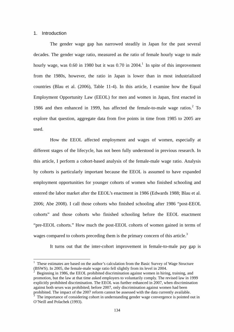
1. Introduction

The gender wage gap has narrowed steadily in Japan for the past several

decades. The gender wage ratio, measured as the ratio of female hourly wage to male

hourly wage, was 0.60 in 1980 but it was 0.70 in 2004.1 In spite of this improvement

from the 1980s, however, the ratio in Japan is lower than in most industrialized

countries (Blau et al. (2006), Table 11-4). In this article, I examine how the Equal

Employment Opportunity Law (EEOL) for men and women in Japan, first enacted in

1986 and then enhanced in 1999, has affected the female-to-male wage ratios.2 To

explore that question, aggregate data from five points in time from 1985 to 2005 are

used.

How the EEOL affected employment and wages of women, especially at

different stages of the lifecycle, has not been fully understood in previous research. In

this article, I perform a cohort-based analysis of the female-male wage ratio. Analysis

by cohorts is particularly important because the EEOL is assumed to have expanded

employment opportunities for younger cohorts of women who finished schooling and

entered the labor market after the EEOL’s enactment in 1986 (Edwards 1988; Blau et al.

2006; Abe 2008). I call those cohorts who finished schooling after 1986 “post-EEOL

cohorts” and those cohorts who finished schooling before the EEOL enactment

“pre-EEOL cohorts.” How much the post-EEOL cohorts of women gained in terms of

wages compared to cohorts preceding them is the primary concern of this article.3

It turns out that the inter-cohort improvement in female-to-male pay gap is

1 These estimates are based on the author’s calculation from the Basic Survey of Wage Structure (BSWS). In 2005, the female-male wage ratio fell slightly from its level in 2004. 2 Beginning in 1986, the EEOL prohibited discrimination against women in hiring, training, and promotion, but the law at that time asked employers to voluntarily comply. The revised law in 1999 explicitly prohibited discrimination. The EEOL was further enhanced in 2007, when discrimination against both sexes was prohibited; before 2007, only discrimination against women had been prohibited. The impact of the 2007 reform cannot be assessed with the data currently available. 3 The importance of considering cohort in understanding gender wage convergence is pointed out in O’Neill and Polachek (1993).

135

rather limited once educational attainment is controlled for. Therefore, the obvious

causes for the narrowing overall gender wage gap are changes in the educational

composition of the workforce. Significant changes in worker composition took place in

the Japanese labor market from the 1980s to the 2000s. Among regular, full-time

employees, increasing educational attainment and “aging” occurred during this period

for both men and women.4 It is shown that the compositional changes in education

explain a non-negligible portion of the improvement in the gender wage ratio. The

results imply that the narrowing gap due to changes in wage structure (higher pay

growth for women than for men after EEOL) may have been limited.

2. Data

I use aggregate data of the Basic Survey of Wage Structure (BSWS) for years

1985, 1990, 1995, 2000, and 2005.5 The BSWS is a survey of earnings and hours,

conducted every year, by the Ministry of Health and Welfare. It is the most widely used

data source of wages in empirical studies of the Japanese labor market. The published

data I use contain cell-mean data of wages, hours, bonuses, and tenure, along with the

estimated number of workers for each cell, where the cell is defined by sex, age group

(5-year interval), and education (4 levels). The hourly wage rates for men and women

are calculated by dividing monthly base earnings (shoteinai kyuyo) by monthly hours

(shoteinai-jitsu rodo jikan). Hours here do not include overtime hours.6

4 Regular, full-time workforce is the set of workers whose employment contract does not set a fixed term length and, in most cases, whose regular work schedules are 40 hours per week. 5 It is still difficult to use microdata of survey data collected by the Japanese government for research purposes. A recent study by Kambayashi et al. (2007) uses microdata of BSWS and contains a detailed description of the BSWS survey method. 6 I performed similar analysis reported below using a wage measure that includes bonuses and overtime hours. The results are generally similar to the ones reported below.

136

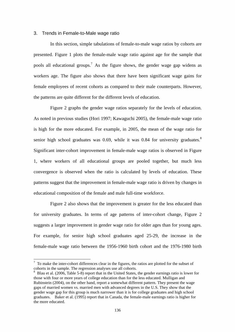
3. Trends in Female-to-Male wage ratio

In this section, simple tabulations of female-to-male wage ratios by cohorts are

presented. Figure 1 plots the female-male wage ratio against age for the sample that

pools all educational groups.7 As the figure shows, the gender wage gap widens as

workers age. The figure also shows that there have been significant wage gains for

female employees of recent cohorts as compared to their male counterparts. However,

the patterns are quite different for the different levels of education.

Figure 2 graphs the gender wage ratios separately for the levels of education.

As noted in previous studies (Hori 1997; Kawaguchi 2005), the female-male wage ratio

is high for the more educated. For example, in 2005, the mean of the wage ratio for

senior high school graduates was 0.69, while it was 0.84 for university graduates.8

Significant inter-cohort improvement in female-male wage ratios is observed in Figure

1, where workers of all educational groups are pooled together, but much less

convergence is observed when the ratio is calculated by levels of education. These

patterns suggest that the improvement in female-male wage ratio is driven by changes in

educational composition of the female and male full-time workforce.

Figure 2 also shows that the improvement is greater for the less educated than

for university graduates. In terms of age patterns of inter-cohort change, Figure 2

suggests a larger improvement in gender wage ratio for older ages than for young ages.

For example, for senior high school graduates aged 25-29, the increase in the

female-male wage ratio between the 1956-1960 birth cohort and the 1976-1980 birth

7 To make the inter-cohort differences clear in the figures, the ratios are plotted for the subset of cohorts in the sample. The regression analyses use all cohorts. 8 Blau et al. (2006, Table 5-8) report that in the United States, the gender earnings ratio is lower for those with four or more years of college education than for the less educated. Mulligan and Rubinstein (2004), on the other hand, report a somewhat different pattern. They present the wage gaps of married women vs. married men with advanced degrees in the U.S. They show that the gender wage gap for this group is much narrower than it is for college graduates and high school graduates. Baker et al. (1995) report that in Canada, the female-male earnings ratio is higher for the more educated.

137

cohort is 0.018. For senior high school graduates aged 40-44, the increase from the

1941-1945 birth cohort to the 1961-1965 birth cohort is 0.097.

The patterns of gender wage ratio by education imply that the EEOL has had

differential impacts on women’s wages and employment. It is known that the EEOL

advanced the regular employment of post-EEOL cohorts of university graduate women

at young ages but did not increase regular employment for less-educated women or for

university graduate women of pre-EEOL cohorts (Abe 2008). Table 1 shows the regular

employment ratio (the ratio of the number of regular employees to population) for the

cohorts of women, where cohort is defined by education and birth year. It is clear that

the regular employment ratio of women is at a similar level for the pre-EEOL cohorts of

all education groups, while a large increase in the regular employment ratio is observed

for young women with university education. Figure 2, on the other hand, indicates that

wage gains (compared with male employees of the same cohort with the same level of

education) are greater for the less-educated group and pre-EEOL cohorts. Therefore, the

groups who gained in terms of an increase in regular employment did not gain in terms

of wages, while the groups that did not gain in terms of employment experienced an

increase in relative wages.

4. Regression analysis of gender wage ratios

Now I turn to a regression analysis of cohort-based female-to-male wage ratios,

to quantify the impact of EEOL on the cohort-based gender wage ratio. The regression

equation I estimate has the following form:

βηδ Xratio_wage ac ++= ,

where the dependent variable is the female-male wage ratio, cδ are the effects for

cohort c, and aη are the effects for age. The regressions are estimated by weighted

least squares by using the hours supplied by workers in each cell (men and women) as

138

weights. The results are shown in Table 2. Column (1) of Table 2 reports results for four

education groups pooled together, without including the education dummies. The cohort

effects indicate that the female-to-male wage gap has narrowed (the dependent variable

takes a larger value) for more recent cohorts; the coefficients of cohort dummies are

always higher for more recent cohorts. However, when education dummies are included

(column (2)), the inter-cohort increase is not as significant as in column (1). The

magnitude of the improvement is not as large as in column (1), and the coefficients of

several cohorts are not higher than the cohort born 5 years earlier.

Columns (3) to (6) of Table 2 report regression results estimated separately for

four educational groups. The coefficients of cohort dummies indicate that cohorts of

women born in 1941-1950 gained relative to men of the same cohorts (the cohort born

in 1956-1960 is the base group in the regressions). It is interesting to note that these are

pre-EEOL cohorts. The post-EEOL cohorts, on the other hand, have not gained much

relative to the 1956-1960 birth cohort, for all education groups. The coefficients of

cohort dummies attached to the post-EEOL cohorts are small in magnitude, and many of

them are not statistically different from zero. Some of the point estimates are even

negative. The pattern in cohort effects also shows that inter-cohort improvement is

smaller for junior college and university graduates than for junior high school and

senior high school graduates.

Kawaguchi (2005) finds that the extension in tenure (the length of service at

the employer) is the main cause for improvement in the gender wage ratio between 1990

and 2000. To investigate the extent of such effects in a cohort context, I run regressions

that add the female-to-male average tenure ratio (average female tenure divided by

average male tenure). The results are shown in Table 3. The coefficients of the relative

tenure variable are positive and statistically significant for senior high school and junior

college samples but not for others. The coefficients of cohort dummies are smaller in

139

absolute value than those reported in Table 2 for senior high school and junior college

groups, suggesting that increase in tenure partly explains the inter-cohort convergence.

After including the relative tenure variable, the inter-cohort improvement in the gender

pay ratio is obvious for less-educated, pre-EEOL cohorts.

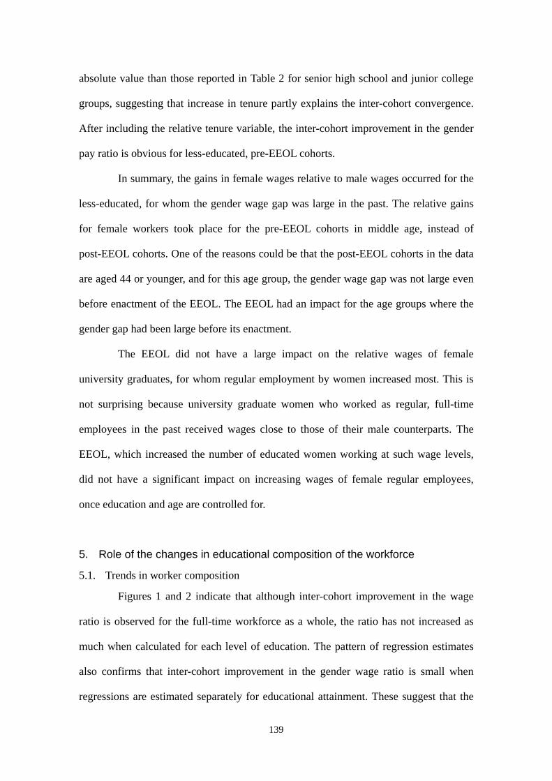
In summary, the gains in female wages relative to male wages occurred for the

less-educated, for whom the gender wage gap was large in the past. The relative gains

for female workers took place for the pre-EEOL cohorts in middle age, instead of

post-EEOL cohorts. One of the reasons could be that the post-EEOL cohorts in the data

are aged 44 or younger, and for this age group, the gender wage gap was not large even

before enactment of the EEOL. The EEOL had an impact for the age groups where the

gender gap had been large before its enactment.

The EEOL did not have a large impact on the relative wages of female

university graduates, for whom regular employment by women increased most. This is

not surprising because university graduate women who worked as regular, full-time

employees in the past received wages close to those of their male counterparts. The

EEOL, which increased the number of educated women working at such wage levels,

did not have a significant impact on increasing wages of female regular employees,

once education and age are controlled for.

5. Role of the changes in educational composition of the workforce

5.1. Trends in worker composition

Figures 1 and 2 indicate that although inter-cohort improvement in the wage

ratio is observed for the full-time workforce as a whole, the ratio has not increased as

much when calculated for each level of education. The pattern of regression estimates

also confirms that inter-cohort improvement in the gender wage ratio is small when

regressions are estimated separately for educational attainment. These suggest that the

140

changes in the educational composition of the workforce should be a key determinant

for the narrowing gap of male and female wages.

Figures 3 and 4 show the share of working hours of regular, full-time

employees supplied by workers of each education-age pair, separately for male and

female workers. The share of university graduates (16 or more years of schooling)

increased for both males and females, while the share of junior high school graduates (9

years of compulsory schooling) fell, especially for men.

The most significant change in worker composition shown in Figures 3 and 4 is

the decline of the share of young workers among women. For example, the share of

hours supplied by workers aged 20-24 was 33 percent in 1985, while the same figure

was 14 percent in 2005. The female, regular, full-time workers used to consist mainly of

senior high school graduate women aged less than 30. By 2005, however, the share of

such workers in the female regular workforce decreased, and the proportion of female

workers with more education and higher ages increased.9 The tabulations of Figures 3

and 4 are for the cross sections of years 1985 and 2005 and are not shown in a format to

follow cohort experiences. They, nevertheless, illustrate the significance of

compositional changes.

What caused the change in educational composition of the regular-full-time

workforce, the set of workers analyzed here? There are two main reasons. One is

obviously the educational attainment of the population has improved.10 The other is

that the regular full-time workforce has become more selective in the sense that it has

become more difficult for the less-educated to engage in regular, full-time work. The

fact that the young men and women lost regular employment during the recession in the

9 It is important to note that this dramatic change is most apparent for full-time employees. For female part-time employees, although educational upgrading took place, the extent is modest compared to full-time employees. 10 The educational composition of cohorts of men and women are shown in Figure A1.

141

1990s has been pointed out (Genda 2003). The loss of regular employment is not

limited to the young, however: it occurred for middle-aged men with less education as

well (Genda 2006; Abe 2008).11

5.2. Role of educational composition

The main focus of the present analysis is the role of educational composition on

the gender wage convergence across cohorts. In order to quantify such effects, I

calculate a counterfactual gender ratio, by setting the educational composition at a fixed

age to be the composition of the cohorts 10 years apart. Let the index of cohort be their

birth year. The counterfactual gender ratio for cohort C of age A is calculated under the

assumption that male and female wages are same as those of cohort C, but the

educational composition is the same as cohort C-10 (those born 10 years earlier) at age

A. Specifically, let asecθ be the proportion of education group e for birth cohort c at

age a for sex s, awsec be the wage rate for education e for cohort c at age a for sex s,

and let sex subscripts be M for male and F for female. Then, the actual female-male

wage ratio for cohort c at age a is

∑∑

⋅

⋅=

eacFeFeca

eacMeMeca

ac w

wRatio

,,

,,

, θ

θ.

The counterfactual wage ratios of cohort c at age a are

∑∑

−

−

⋅

⋅=

eacFeFeca

eacMeMeca

ac w

wECRatio

,10,

,10,

,_θ

θ,

11 Note that Figures 3 and 4 show shares in hours supplied, instead of number of workers. This is motivated by the fact that the hourly wages used in this paper are weighted averages of hourly wage rates of individual workers, with hours supplied by individual workers are used as the weight. This is the only measure of hourly wages available using aggregate data. Shares in hours supplied are determined by hours supplied by individual workers as well as number of workers. In fact, working hours changed significantly from 1985 to 2005, and the pattern of changes differs across educational groups. However, its effect on gender pay ratios is not large because the pattern of changes is similar between male and female workers within each education group.

142

∑∑

+

+

⋅

⋅=

eacFeFeca

eacMeMeca

ac w

wLCRatio

,10,

,10,

,_θ

θ,

where acECRatio ,_ is the ratio calculated from the weight with the cohort born 10

years earlier than cohort c, and acLCRatio ,_ is the ratio calculated with the weight of

the cohort born 10 years later. The differences between the actual ratio and the

counterfactual are the differences in weight (i.e. asecθ ’s). Note that acECRatio ,_ and

acRatio ,10− differ only in w’s, because for these two, θ ’s are the same. If acECRatio ,_

is close to acRatio ,10− , it means awsec and acsew ,10, − are “close” and the impact of

composition (θ ’s) is the main reason for the changes in 10−cRatio to cRatio . The

results of this decomposition are shown in Figure 5 for the two cohorts (c equals the

1951-1955 and 1961-1965 birth cohorts). The solid lines are the actual gender wage

ratios for the three cohorts that are 10 years apart in their birth years. The dotted lines

are the counterfactual gender wage ratios ( ac,CRatio_E and ac,CRatio_L ). In the case of

Figure 5A, actual gender pay ratios for cohorts born 1941-1945, 1951-1955, and

1961-1965 are shown in solid lines, and counterfactual gender ratios are shown in

dotted lines: these counterfactuals are calculated using average male and female wages

for the 1951-1955 cohort but using the educational composition of working hours for

the 1941-1945 cohort and the 1961-1965 cohort, respectively.12 If the dotted line and

the solid line of another cohort are located closely, changes in educational composition

explain most of the inter-cohort change (i.e. the actual changes in the wage ratio occurs

mostly because of the compositional change); if not, changes in wage structure

contributed to the narrowing gap. The pattern in Figure 5 indicates that the much of the 12 The solid lines in the left portion of Figure 5A are the same as those in the right portion of Figure 5B, since they are the actual gender ratio profiles for the 1951-1955 and 1961-1965 cohorts. The locations of the two dotted lines are somewhat different, implying that the choice of wage profiles to calculate the counterfactual yields different results.

143

improvement for the younger cohorts is attributed to compositional changes, but that for

the older cohorts is not.

6. Discussion

The analysis in this article shows that the female-to-male wage ratios increased

for more recent cohorts. At the same time, it suggests that a large part of inter-cohort

improvement is attributable to compositional changes in the full-time workforce. It is

interesting to note that improvement in the gender pay ratio occurred for the group for

whom regular employment of women did not grow. University graduate women

experienced increases in full-time employment, but their wages did not rise much

relative to male university graduates. Young women with junior or senior high school

education became less likely to work in full-time employment. However, wages of

female junior and senior high school graduates, especially for older groups, seem to

have improved relative to their male counterparts.

How do the results above differ from other studies that examine the gender

wage gap in Japan? Hori (1998) uses microdata of the BSWS in 1986 and 1994 to

perform the Juhn-Murphy-Pierce type decomposition (Juhn et al. 1991) similar to the

analysis done by Blau and Kahn (1997) for the United States. Kawaguchi (2005) uses

microdata of the BSWS in 1990 and 2000 to perform the JMP decomposition. These

two studies, while using a similar technique, reach rather different conclusions.

Specifically, Hori concludes that the unobserved effect is the most significant cause for

the decline in the gender wage gap and does not find that the increase in tenure

contributed to the narrowing of the gender wage gap. Kawaguchi, on the other hand,

finds that extension of tenure is the most significant cause for convergence. The timing

of the data used in the two studies is 6 years apart, which may explain the different

results. For one, if the impacts of EEOL materialize as time passes, the pattern of the

144

gender wage gap may differ depending on the phases of that development. Alternatively,

it is possible that the compositional changes in workforce that took place between these

years have contributed to the differing results.

Kawaguchi and Naito (2006) use microdata of Employment Status Survey and

employ a bound technique to find the upper and lower bounds for the gender wage

convergence. Kawaguchi and Naito account for composition in modeling participation

decision. However, none of these analyses is based on cohorts, so existence (or

non-existence) of cohort effects has not been identified.

Young, educated women increased participation in full-time employment after

the enactment of EEOL. However, the EEOL may have benefited another group of

women (older women with less education) in terms of wages. The long-term

consequences of EEOL impacts are a topic for further study.

What are the implications for the above results for labor supply of women in

Japan? The fact that the wage increases of women (compared to their male counterparts)

occurred for the group for whom full-time employment did not grow implies that

full-time labor supply of women is not likely to respond to contemporaneous wages. For

example, if the increases in regular employment of young, educated women are

responses to rising wages, wages for educated women of post-EEOL cohorts should

have increased at the time when such employment rose. The fact that it did not suggests

that regular employment of women does not respond much to contemporaneous wages.

145

References

Abe, Yukiko (2008) “A cohort analysis of male and female labor supply in Japan.”

Mimeo, Hokkaido University.

Baker, Michael, Dwayne Benjamin, Andree Cegep, and Mary Grant (1995) “The

Distribution of the Male/Female Earnings Differential, 1970-1990.” Canadian

Journal of Economics 28:3, 479-501.

Blau, Francine D., Marianne A. Ferber, and Anne E. Winkler (2006) The Economics of

Women, Men, and Work, Fifth Edition, Pearson, Prentice Hall.

Blau, Francine D. and Lawrence M. Kahn (1997) “Swimming Upstream: Trends in the

Gender Wage Differential in the 1980s.” Journal of Labor Economics, 15:1, Part

1, 1-42.

Edwards, Linda (1988) “Equal Employment Opportunity in Japan: A View from the

West.” Industrial and Labor Relations Review 41:2, 240-250.

Genda Yuji (2003) Who Really Lost Jobs in Japan?: Youth Employment in an Aging

Japanese Society, In: Labor Markets and Firm Benefit Policies in Japan and the

United States, (eds) Seiritsu Ogura, Toshiaki Tachibanaki, and David Wise, The

University of Chicago Press, Chicago London, 103-133.

Genda, Yuji (2006) “Inequality of middle-aged non-workers” (Chuunenrei mugyosha

kara mita kakusa mondai) In: Henka suru shakaino hubyoudo [Inequality in a

changing society] ed. Sawako Shirahase, University of Tokyo Press, 79-104 (in

Japanese).

Hori, Haruhiko (1998) “Narrowing Gap: Trends in the Gender Wage Differential in

Japan” [Danjyokan chingin kakusa no shukusho keiko to sono yoin] Japanese

Journal of Labour Studies 456, 41-51 (in Japanese).

Juhn, Chinhui, Kevin M. Murphy, and Brooks Pierce (1991) “Accounting for the

Slowdown in Black-White Wage Convergence.” In: Workers and Their Wages,

146

ed. Marvin Kosters, Washington, DC: AEI Press 107-43.

Kambayashi, Ryo; Daiji Kawaguchi and Izumi Yokoyama (2007) “Wage Distribution in

Japan: 1989-2003.” Canadian Journal of Economics, forthcoming.

Kawaguchi, Akira (2005) “Factors for the narrowing male-female wage gap in the

1990s” [1990 nendai ni okeru Danjo-kan Chingin Kakusa Shukusho no Yoin],

Economic Analysis [Keizai Bunseki], Vol.175, Cabinet Office of Japan, Tokyo

(in Japanese).

Kawaguchi, Daiji, and Hisahiro Naito (2006) “The Bound Estimate of the Gender Wage

Convergence under Employment Compositional Change,” ESRI Discussion

Paper 161.

Mulligan, Casey and Yona Rubinstein (2004) “The closing of the gender gap as a Roy

model illusion.” NBER Working Paper 10892.

O’Neill, June, and Solomon Polachek (1993) “Why the Gender Gap in Wages Narrowed

in the 1980s.” Journal of Labor Economics, 11:1, Part 1, 205-228.

147

Tables and Figures Table 1: Regular Employment Ratio of Women, by Education

Education birth year20-24 25-29 30-34 35-39 40-44 45-49 50-54

Junior High 1938-1942 0.230 0.2401943-1947 0.213 0.255 0.2271948-1952 0.188 0.242 0.237 0.1791953-1957 0.171 0.221 0.224 0.1841958-1962 0.182 0.180 0.183 0.1441963-1967 0.263 0.199 0.158 0.1361968-1972 0.269 0.166 0.1231973-1977 0.217 0.123

Senior High 1938-1942 0.229 0.2381943-1947 0.231 0.265 0.2371948-1952 0.206 0.254 0.263 0.2071953-1957 0.207 0.241 0.250 0.2311958-1962 0.319 0.236 0.237 0.2191963-1967 0.652 0.379 0.250 0.2141968-1972 0.665 0.373 0.2281973-1977 0.560 0.327

Junior College 1938-1942 0.265 0.2661943-1947 0.268 0.261 0.2741948-1952 0.265 0.287 0.294 0.2651953-1957 0.281 0.289 0.295 0.2781958-1962 0.530 0.308 0.271 0.2701963-1967 0.744 0.504 0.309 0.2641968-1972 0.810 0.518 0.3201973-1977 0.718 0.475

University 1938-1942 0.339 0.3101943-1947 0.295 0.285 0.3321948-1952 0.333 0.328 0.339 0.3041953-1957 0.334 0.341 0.345 0.3131958-1962 0.505 0.390 0.338 0.3291963-1967 0.733 0.620 0.426 0.3601968-1972 0.826 0.616 0.4201973-1977 0.723 0.559

Note: The figures are the number of regular workers (not including executives) divided by population.Source: Employment Status Survey (1987, 1992, 1997, and 2002), published version

Age group

148

Table 2: Regression analysis of female-to-male wage ratiosDependent variable: Female-male wage ratio in base hourly wage (excluding bonuses)

(1) (2) (3) (4) (5) (6)Education level of thesample ALL ALL Junior High Senior High Junior College University

Dummy for born -0.115 ** -0.068 ** -0.089 ** -0.076 ** -0.036 * -0.045 1941-1945 (0.034) (0.014) (0.005) (0.013) (0.016) (0.024)Dummy for born -0.081 * -0.049 ** -0.062 ** -0.045 ** -0.047 ** -0.050 1946-1950 (0.032) (0.010) (0.005) (0.011) (0.012) (0.025)Dummy for born -0.046 -0.027 ** -0.032 ** -0.028 ** -0.036 * -0.011 1951-1955 (0.031) (0.010) (0.005) (0.009) (0.015) (0.019)Dummy for born 0.020 0.014 0.013 0.022 0.014 -0.006 1961-1965 (0.029) (0.009) (0.016) (0.011) (0.010) (0.015)Dummy for born 0.031 0.020 * 0.016 0.026 * 0.022 * -0.001 1966-1970 (0.029) (0.008) (0.010) (0.012) (0.010) (0.014)Dummy for born 0.038 0.022 * 0.031 ** 0.028 * 0.030 ** -0.003 1971-1975 (0.030) (0.010) (0.009) (0.010) (0.009) (0.013)Dummy for born 0.043 0.016 0.063 ** 0.028 * 0.027 * -0.012 1976-1980 (0.032) (0.014) (0.010) (0.013) (0.010) (0.013)Dummy for Age 20-24 0.183 ** 0.206 ** 0.115 ** 0.227 ** 0.202 ** 0.166 **

(0.031) (0.012) (0.017) (0.013) (0.014) (0.020)Dummy for Age 25-29 0.149 ** 0.151 ** 0.065 ** 0.171 ** 0.166 ** 0.127 **

(0.032) (0.010) (0.013) (0.012) (0.012) (0.020)Dummy for Age 30-34 0.097 ** 0.098 ** 0.033 ** 0.111 ** 0.108 ** 0.088 **

(0.031) (0.008) (0.008) (0.009) (0.011) (0.020)Dummy for Age 35-39 0.043 0.043 ** 0.020 ** 0.040 ** 0.055 ** 0.048 *

(0.030) (0.009) (0.004) (0.009) (0.012) (0.020)Dummy for Age 45-49 -0.018 -0.018 * 0.003 -0.016 -0.018 -0.043

(0.027) (0.009) (0.004) (0.009) (0.015) (0.027)Dummy for Age 50-54 -0.017 -0.018 0.025 ** -0.023 -0.018 -0.046 *

(0.029) (0.012) (0.003) (0.013) (0.023) (0.021)Junior High -0.047 **

(0.009)Junior College 0.106 **

(0.005)University 0.140 **

(0.006)Constant 0.701 ** 0.647 ** 0.618 ** 0.636 ** 0.744 ** 0.810 **

(0.031) (0.010) (0.005) (0.010) (0.010) (0.027)

Observations 124 124 31 31 31 31R-squared 0.74 0.97 0.98 0.99 0.99 0.96

Robust standard errors in parentheses.* significant at the 5% level; ** significant at the 1% level.The wage measure of the dependent variable does not include bonuses.Regressions are estimated by weighted least squares, using the hours worked by workersin each cell as weights.The base group for cohort dummies is the cohort born in 1956-60.The base group for age dummies is those aged 40-44.The base group for education is senior high school graduates.

Source: Author's calculation from the BSWS.

149

Table 3: Regression analysis of female-to-male wage ratios (includes tenure ratio as regressor)Dependent variable: Female-to-male wage ratio in base hourly wage (excluding bonuses)

(1) (2) (3) (4)Education level of thesample Junior High Senior High Junior College University

Dummy for born -0.100 ** -0.042 ** 0.017 -0.042 1941-1945 (0.012) (0.011) (0.012) (0.025)Dummy for born -0.071 ** -0.022 * -0.012 -0.050 1946-1950 (0.011) (0.009) (0.006) (0.026)Dummy for born -0.036 ** -0.014 -0.012 -0.013 1951-1955 (0.007) (0.007) (0.009) (0.020)Dummy for born 0.015 0.013 0.015 * -0.012 1961-1965 (0.015) (0.009) (0.006) (0.017)Dummy for born 0.013 0.013 0.014 -0.013 1966-1970 (0.010) (0.013) (0.007) (0.017)Dummy for born 0.022 0.017 0.041 ** -0.015 1971-1975 (0.012) (0.011) (0.006) (0.018)Dummy for born 0.047 ** 0.033 0.038 ** -0.021 1976-1980 (0.015) (0.016) (0.006) (0.015)Dummy for Age 20-24 0.137 ** 0.143 ** 0.114 ** 0.132 **

(0.023) (0.019) (0.014) (0.033)Dummy for Age 25-29 0.080 ** 0.098 ** 0.086 ** 0.104 **

(0.011) (0.019) (0.013) (0.029)Dummy for Age 30-34 0.040 ** 0.063 ** 0.049 ** 0.075 **

(0.008) (0.013) (0.011) (0.024)Dummy for Age 35-39 0.023 ** 0.024 ** 0.026 * 0.042

(0.004) (0.008) (0.010) (0.021)Dummy for Age 45-49 0.004 -0.016 ** -0.008 -0.033

(0.005) (0.004) (0.007) (0.026)Dummy for Age 50-54 0.028 ** -0.032 ** -0.031 ** -0.041

(0.004) (0.007) (0.007) (0.021)tenure_ratio -0.060 0.278 ** 0.400 ** 0.148

(0.049) (0.067) (0.056) (0.081)Constant 0.663 ** 0.453 ** 0.437 ** 0.701 **

(0.041) (0.044) (0.042) (0.052)

Observations 31 31 31 31R-squared 0.985 0.996 0.995 0.960

Notes:Robust standard errors in parentheses.* significant at the 5% level; ** significant at the 1% level.The wage measure of the dependent variable does not include bonuses.Regressions are estimated by weighted least squares, using the hours worked by workersin each cell as weights.The base group for cohort dummies is the cohort born in 1956-60.The base group for age dummies is those aged 40-44.The base group for education is senior high school graduates.

Source: Author's calculation from the BSWS.

150

Figure 1: Female-Male wage ratio for cohorts

Figure 2: Female-Male wage ratio for cohortsBy education

.4

.6

.8

1.4

.6

.8

1

20 30 40 50 60 20 30 40 50 60

Junior High Senior High

Junior College University

1931-1935 1941-1945 1951-1955 1961-1965

1971-1975

Female-Male Wage Ratio

Age

Source: BSWS (published version)

.4

.6.8

1Female-Male Wage Ratio

20 30 40 50 60Age

1931-1935 1941-1945 1951-1955 1961-1965

1971-1975

Source: BSWS (published version)

151

Figure 3: Changes in hours share from 1985 to 2005Male regular employees

Source: Author's calculation from the Basic Survey of Wage Structure (published version).

0.05

.1

.15

.2

.25

20-24 25-29 30-34 35-39 40-44 45-49 50-54 55-59

Hours share of male regular employees in 1985

Junior High Senior High

Junior College University

0.05

.1

.15

.2

.25

20-24 25-29 30-34 35-39 40-44 45-49 50-54 55-59

Hours share of male regular employees in 2005

Junior High Senior High

Junior College University

152

Figure 4: Changes in hours share from 1985 to 2005Female regular employees

Source: Author's calculation from the Basic Survey of Wage Structure (published version).

0.05

.1

.15

.2

.25

20-24 25-29 30-34 35-39 40-44 45-49 50-54 55-59

Hours share of female regular employees in 2005

Junior High Senior High

Junior College University

0.05

.1.15

.2

.25

20-24 25-29 30-34 35-39 40-44 45-49 50-54 55-59

Hours share of female regular employees in 1985

Junior High Senior High

Junior College University

153

Figure 5: Effects of educational composition on gender wage ratio

Source: Author's calculation from the Basic Survey of Wage Structure (published version).

.5

.6.7

.8

.9

1

20 25 30 35 40 45Age

actual, 1961-1965 actual, 1951-1955 actual, 1971-1975

weights of 1951-1955 weights of 1971-1975

B. Base group: 1961-1965 cohort

.5.6

.7.8

.9

1

30 35 40 45 50 55Age

actual, 1951-1955 actual, 1941-1945 actual, 1961-1965

weights of 1941-1945 weights of 1961-1965

A. Base group: 1951-1955 cohort

154

Figure A1: Educational distribution by cohorts

Source: Employment Status Survey, 2002 (published version).

Men

0

0.1

0.2

0.3

0.4

0.5

0.6

0.7

0.8

0.9

1

1978-1982

1973-1977

1968-1972

1963-1967

1958-1962

1953-1957

1948-1952

1943-1947

1938-1942

Birth year

Fra

ction

Univ

Junior College

Senior High

Junior High

Women

0

0.1

0.2

0.3

0.4

0.5

0.6

0.7

0.8

0.9

1

1978-1982

1973-1977

1968-1972

1963-1967

1958-1962

1953-1957

1948-1952

1943-1947

1938-1942

Birth year

Fra

ction

Univ

Junior College

Senior High

Junior High