chapter 6 analysis of quantitative data and discussion on...

CHAPTER 6

ANALYSIS OF QUANTITATIVE DATA

AND DISCUSSION ON TRANSIT TIME

AND SHIPMENT DATA

24

CHAPTER6

ANALYSIS OF QUANTITATIVE DATA AND DISCUSSION ON TRANSIT TIME AND SHIPMENT DATA

Quantitative data was collected by monitoring the movement of the actual shipments as

they move through the supply cbafin. Based on the dates that were logged on to the

tracking sheet the number of days required to complete individual steps were calculated.

This analysis was done for CFS stuffed containers, ICD stuffed containers, factory

stuffed containers and import containers from the discharge port to CFS Patparganj. The

data thus collected was analyzed in the following manner

A) Preparation of descriptive statistics for individual samples

B) Effect of lead time variability, measured through the standard deviation, on the ROP

equation of inventory management, for the different supply chain

C) Study of Full Container Loads stuffed at factory, as a sample case to study the

following

• Ability of the chain to provide on-time delivery.

• Variability in activity lead-times between various stages of the supply chain

• Correlation between total lead time to time taken up to containerization

Description of columns

Customs Clearance: The number of days from carting of cargo to the custom bonded area

to custom clearance of the shipment calculated from the difference in dates of the events

Containerization: The number of days from custom clearance to the containerization of

the shipment at the bonded area calculated from the difference in dates of the events

Railing: The number of days from containerization to railing from railhead calculated

from the difference in dates of the events

Sailing: The number of days from railing to sailing of the container from port of loading

calculated from the difference in dates of the events

Total: The total number of days taken by a shipment to sail from the port from the date

cargo was carted at the CFS, calculated from the difference in dates of the events

Emptv placement at factorv: Number of days required to place empty container at factory

for factory stuffing af\er receipt of documents for customs clearance.

Page 125

6.1 OBSERVATIONS ON STUDY OF TRANSIT TIME OF SHIPMENTS

BETWEEN DELHI AND PORT OF NHAVA SHEVA

6.1.1 Sample A: LCL Consolidation Cargo

DESCRIPTION OF SAMPLE

• Type of cargo: less than container loads (LCL)

• Place of custom clearance: CFS Patparganj, Delhi '

• Place of containerization: CFS Patparganj, Delhi

• Rail head: ICD Tuglakabad

• Custom documentation type: Various (duty drawback, duty entitlement passbook

scheme, white shipping bill)

• Mode of transport

• CFS to railhead: By road. Railhead to port: By rail

• Sample size: 26 shipments

• Sample period: June 2000 to October 2000

Table 27- Shipment data for LCL s

MEASURE

AVERAGE

STD.DEVIATION

MODE

MEDIAN

MAX

MIN

VARIANCE

A)

CUSTOM

CLEARANCE

4.19

4.17

1

3

15

1

17.35

hipments

B)

CONTAINERISATION

8.31

9.81

1.00

2.00

30.00

0.00

96.14

C)

RAILING

2.00

2.95

1.00

1.00

16.00

1.00

8.72

D)

SAILING

7.15

1.67

8

8

9

3

2.78

E)

TOTAL

15.38

7.88

12

12.50

39.00

8.00

62.09

UNIT OF MEASUREMENT: DAYS

Page 126

6.1.2 Sample B: Full Container Loads Containerized at ICD


• Type of cargo: Full container loads (FCL)

• Place of custom clearance: ICD Tuglakabad, Delhi

• Place of containerization: ICD Tuglakabad

• Rail head: ICD Tuglakabad

• Mode of transport: Factory container yard by road. Railhead to port: by rail

• Sample size 16 shipments

• Sample period: August 2000 to December 2000 ,

STATISTICAL OBSERVATIONS

Table 28 - Shipment Data for ICD Shipments

MEASURE

Max Value

Min Value

Mode

Median

Average

Standard Dev.

Variance

A)CUSTOMS

CLEARANCE

6

0

3

3

2.89

1.45

2.12

B)RAILING

OF

CONTAINER

6

0

1

2

2.18

1.47

2.16

C)SAIL1NG

OF

CONTAINER

15

3

6

6

7.06

3.14

9.85

D) TOTAL

NO. OF DAYS

23

8

10

10

12.18

4.27

18.23


Page 127

6.1.3 Sample C: Full Container Loads Containerized At Factory


Type of cargo: Full container loads (FCL)

Place of custom clearance: ICD Tuglakabad, Delhi

Place of containerization: Shipper's factory 30kms from container yard

Rail head: ICD Tuglakabad

Mode of transport: Container yard to factory and back to container yard by road

Railhead to port: By rail

Sample size 52 shipments

Sample period: Aug. 2002 to Sept. 2002

STATISTICAL OBSERVATIONS

Table 29- Shipment Data for Factory Stuffed FCLs

Average

Min Value

Max Value

STD.

Deviation

Median

Mode

Variance

Empty Placement at

Factory

1.10

0.00

2.00

0.37

1.00

1.00

0.13

Custom

Clearance

1.94

0.00

4.00

0.998

2.00

1.00

1.00

Railing

0.77

0.00

2.00

0.47

1.00

1.00

0.22

Arrival at

POD

2.85

2.00

6.00

1.29

2.00

2.00

1.66

Sailing

4.58

2.00

24.00

4.37

4.00

2.00

19.07

Total

Days

11.27

6.00

34.00

5.27

10.050

10.00

28.11


Page 128

6.1.4 Sample D: Import Shipments Up to ICD Delhi from Nava Sheva and Mumbai


Type of cargo: Full container loads (FCL) and FCLs of consolidated LCLs

Place of delivery: ICD Tuglakabad, Delhi

Place of de -containerization: ICD Tuglakabad

Rail head: ICD Tuglakabad

Port to inland container depot: by rail

Sample size 26 shipments

Sample period: Jan 2000 to July 2000

Table 30- Shipment Data for Import Shipments

MEASURE

Min

Max

Mode

Median

Average

Standard Deviation

Skew

Variance

RAILING

1.00

16.00

2.00

3.00

5.63

4.8

1.05

23.04

ARRIVAL

DESTINATION

1.00

10.00

2.00

3.50

3.96

2.2

1.02

4.84

TOTAL UPTO

DESTINATION

3.00

22.00

4.00

6.00

9.58

6.29

0.75

39.56



A) Deviation of actual arrival date of shipment from planned arrival.

B) The number of days from discharge of container from vessel at arrival port to onward

railing for inland container terminal, calculated from the difference in dates of the events

C) The number of days from railing from port to arrival at ICD, calculated from the

difference in dates of the events

D) The total number of days from arrival of container at port of discharge to arrival at

ICD, calculated from the difference in dates of the events

Page 129

6.2 SIGNIFICANCE OF SUPPLY CHAIN PERFORMANCE TO INVENTORY

MANAGEMENT

Firms seek to keep inventory carrying costs at a minimum and follow the J.l.T (Just in

time) concept for inventory management. In order to meet the challenges of the J.l.T

system the supply chain needs to deliver consistent performances. We wish to check the

performance of the international supply chain in meeting the requirements of the J.l.T

concept.

Firms also use BENCHMARKING and monitor performance using techniques such as

'BALANCE SCORE CARD^' and 'PERFORMANCE MATRICES ' Benchmarking is a

process of identifying , understanding and adapting outstanding practices to help

organizations improve their performance. As companies develop their supply chain

efficiency they are able to measure their own progress from year to year. However they

are unable to measure their progress against that of other companies in the same sector.

Benchmarking results in the defining of performance matrices that are used for measuring

performance. In the field of logistics commonly used performance matrices are follows

• Percent of sales for total logistics cost

8% to 10%

• World class companies error rates on orders shipped

Less than 1 per 1,000

• World class companies inventory turnover rate

over 20

• World class companies total order cycle time

4 to 6 days

• Percent of sales increase if stock outs were eliminated

10% to 14%

• "Best-In-Class" percentage of on-time delivery

98%

• "Best-In-Class" percentage of order completeness

98%

Page 130

6.2.1 Reorder Point (ROP) Equation.

It is not enough to know how much to order; it is also important to know at what point

to order. The ROP model determines when to order. When the quantity on hand drops to a

predetermined amount, it is time to reorder. This amount includes expected demand during

lead time and usually some safety stock to reduce the probability of a stock-out.

For a daily demand (d) and lead time (LT), reorder point (ROP) is defined as

(d)(LT) = dLT

ROP = dLT

We must at least have enough inventories to cover the lead-time demand. Since the lead-

time demand may vary, it is advisable to carry some extra inventories (safety stock) on top

of the lead-time demand.

The amount of safety stock depends on a which is the standard deviation of the lead-

time demand. The safety stock is a multiple of a or zo where z is the multiple determined

from the standard normal table. For example, if the objective is to meet the demand during

90% of the lead-time cycles, the z value would be approximately 1.28 and the safety stock

would be 1.28a. 90% here is called the service level. Hence, ROP is established above the

average lead-time demand (dLT) by incorporating safety stocks. The complete ROP

equation becomes

ROP = dLT + dza

For a performance level of 98% on time delivery, which is the accepted benchmark, Z

would be 2.058

Therefore

ROP =dLT + 2.058da

Page 131

ILLUSTRATION

Table 31- Review of Shipment Data through ROP Equation.

SAMPLE SIZE 52 16 26 26

AVERAGE LEAD TIME 11.27 1218 15.38 9.58

POPULATION STND. DEVIATION 0.73 1.07 1.55 1.23

INCREMENTAL LEAD TIME 1.50 220 3.18 254

, % INCREASE FOR VARIABLE LEAD TIME 13.35 18.04 20.68 26 50

EXPORTS FCL FACTORY STUFFING EXPORTS FCL ICO STUFFING LCLCONSILDATION IMPORTS LC AND FCL ROP =dLT • 2.058d$

We use the standard deviations for total lead-time between port and container yard to

study the effect of the variability of the supply chain on the ROP equation of inventory

management. Since the standard deviations measured are standard deviations of the

samples, the values were divided by the square root of the sample size to arrive at the

standard deviation of the population. The calculated population standard deviations are

very near the user estimated standard deviation of 1.5 calculated using the Gantt Charts.

Implications

In order to meet the accepted standard of delivery accuracy of 98 % given the

performance of the existing supply chain system, Indian industry would have to make

adjustment for lead time by 13.3 to 26.5 %.Since the physical transit time can not be

compressed due to limitations placed by transport infrastructure, one method to reduce

the lead-time would be to increase the frequency of the shipments so as to reduce the time

difference between subsequent shipments in a continuous replenishment inventory

program. Another option would be to maintain a inventory near to the point of

consumption so as to achieve lower lead-times.

It can be inferred that in order to meet the accepted standard of delivery accuracy of 98 %

given the performance of the existing supply chain system, Indian industry would need to

keep either a buffer or pipe line inventory up to 26 % of the reorder point.

Page 132

6.3 HYPOTHESIS TESTING FROM QUANTITATIVE DATA

We wish to check the responsiveness of the supply chain to the requirements of inventory

Management.

The main inventory types are raw material inventories, work-in-process (WIP) inventories

and finished goods inventories. It is important for the firms to know how much inventory

they should carry. If they carry too much inventory, it will be costly. There is holding or

carrying cost for inventories due to the cost of capital (dividends or interest on funds

invested in inventory or the opportunity cost if the company does not borrow money), cost

of storage (warehouse related costs), obsolescence cost (when the items in inventory become

outdated they lose value), insurance and taxes on inventory. On the other hand, if the firms

carry too little, they may encounter stock-outs and lost sales. There is also an order cost

associated with inventories. Preparing the paperwork for purchase orders, communication

costs, handling the delivery of the shipment, and costs associated with various logistics

activities(storage ,inspection etc,) are the cost elements involved in placing and processing

an order.

We wish to examine, if the supply chain for exports from India is able to achieve on time

delivery at 98% accuracy as is the internationally accepted benchmark. To examine this

we take a sample of 52 export shipments. This is a controlled sample of factory stuffed

FCLs, from one single factory and under one specific scheme for export clearance

(clearance under 100 % EOU). For the purpose of hypothesis testing we examine the

ability of the supply chain to be able to maintain a lead-time, at its value at the mode.

We define a shipping window of a lead time of 10-11 days from empty container dispatch

to sailing from port, to test the hypothesis that shipments sail on time 98% of the time.

For the purpose of research the lead time was limited to sailing from port.


We use the sample for factory stuffed FCLs for testing the hypothesis because the

standard deviations (population standard deviation after accounting for sample size) for

this sample was the least, implying that this supply chain was giving the most consistent

performance

Page 133

Table 32- Shipment Data for Hypothesis Testing

Average

Min Value

Max Value

STD.

Deviation

Median

Mode

Variation

Empty Placement at

Factory

1.10

0.00

2.00

0.37

1.00

1.00

0.13

Custom

Clearance

1.94

0.00

4.00

0.998

2.00

1.00

1.00

Railing

0.77

0.00

2.00

0.47

1.00

1.00

0.22

Arrival at

POD

2.85

2.00

6.00

1.29

2.00

2.00

1.66

Sailing

4.58

2.00

24.00

4.37

4.00

2.00

19.07

Total

Days

11.27

6.00

34.00

5.27

10.050

10.00

28.11

UNIT OF MEASUREMENT: DA YS


Empty placement at factory: Number of days required to place empty container at factory

for factory stuffing after receipt of documents for customs clearance.

Customs Clearance: The number of days from carting of cargo to the custom bonded area

to custom clearance of the shipment.

Railing: The number of days from containerization to railing from railhead calculated

from the difference in dates of the events

Arrival at port: The number of days from railing from railhead to arrival at port.

Sailing: The number of days from railing to sailing of the container from port of loading.

Total: The total number of days taken by a shipment to sail from the port, from the date

documents were received for dispatch of empty container to factory.

6.3.1 Ability of the supply chain to achieve 98 % on time delivery

NULL HYPOTHESIS I

It is hypothesized that export shipments are able to achieve on time sailing 98% of the

time.

ALTERNATE HYPOTHESIS

The export shipments are able to achieve on time sailing less than 98% of the time.

Page 134

Since our alternate hypothesis that that the sample proportion is less that the hypothesized

proportion (0.98) we use the left end tail test to test our hypothesis

Z for p=0.98 is -2.054 in case of the left end tail.

At 95% level of confidence,

Z for the above sample is computed at -35.61

Hence null hypothesis is rejected.

6.3.2 Ability of the Supply Chain to Achieve 40% On-Time Delivery

We use the trail and error method to try and find out the level of performance of the

supply chain by checking the performance at 40% on-time delivery.

NULL HYPOTHESIS 2

It is hypothesized that export shipments are able to achieve on time sailing 40% of the

time.

ALTERNATE HYPOTHESIS

The export shipments are able to achieve on time sailing les than 40% of the time

Since our alternate hypothesis that that the sample proportion is less that the hypothesized

proportion (0.40) we use the left end tail test to test our hypothesis

Z for p=0.98 is -2.054.

At 95% level of confidence,

Z for the above sample is computed at -1.64

Hence null hypothesis is accepted.

6.3.3 Ability of the Incoming Supply Chain to Achieve On Time Delivery

We similarly use the sample data of shipments incoming to the container yard from the

port of loading to check the performance of the supply chain for meeting on-time delivery

98% and 40% of the time. The significance was checked at the level of 95%. For the

sample of 26 shipments 'p' was calculated as the ability of the supply chain to arrive at

the median value of the sample at 0.192. The calculated values of z were '-28.17' and

'-.164' for 98% and 40% on-time delivery. Since the calculated value of z was less than

the tabulated value for the left end single tail test, the null hypothesis was rejected for

both the levels.

Page 135

6.3.4 Lead Time Variability at Various Stages in the Supply Chain

We wish to examine further the behavior of the lead times at various stages of the supply

chain using actual shipment data.

We wish to examine if the variation in the lead-times is comparable at all linked steps in

the supply chain process. If there is no difference in the variance in time taken for the

completion of various stages, it would imply that there is synchronization in the supply

chain. Alternately a variation across different stages would imply that there exist different

efficiency levels at different stages which could have a cascading effect on the total

variance of the variance at different stages.

We use the Bartlett test statistic which is designed to test for equality of variances across

groups against the alternative that variances are unequal for at least two groups.

Null Hypothesis HO: Var 1 =Var2=Var3=Var4

Alternate Hypothesis Ha: Var i # Var j , for at least one pair (i, j).

We wish to check variance across following stages

Table 32a- Shipment Data for Hypothesis Testing

Empty Placement at Factory

0.13

Custom Clearance

1.00

Railing

0.22

Arrival at POD

1.66

Sailing

19.07

Total

28.11

We use the above sample to test the multi-variance across the various stages. We test for

homogeneity of variance between the stages.

The results of Bartlett's test for the above sample were as follows:

Sample size 52

Chi Square = 381.80851

P-Value =0

There is very strong evidence against the null hypothesis.

Checking again, excluding this time the lead-time variance for sailing of container we

calculate Chi-square as 94.94, implying strong evidence against null hypothesis.

Hence null hypothesis is rejected.

6

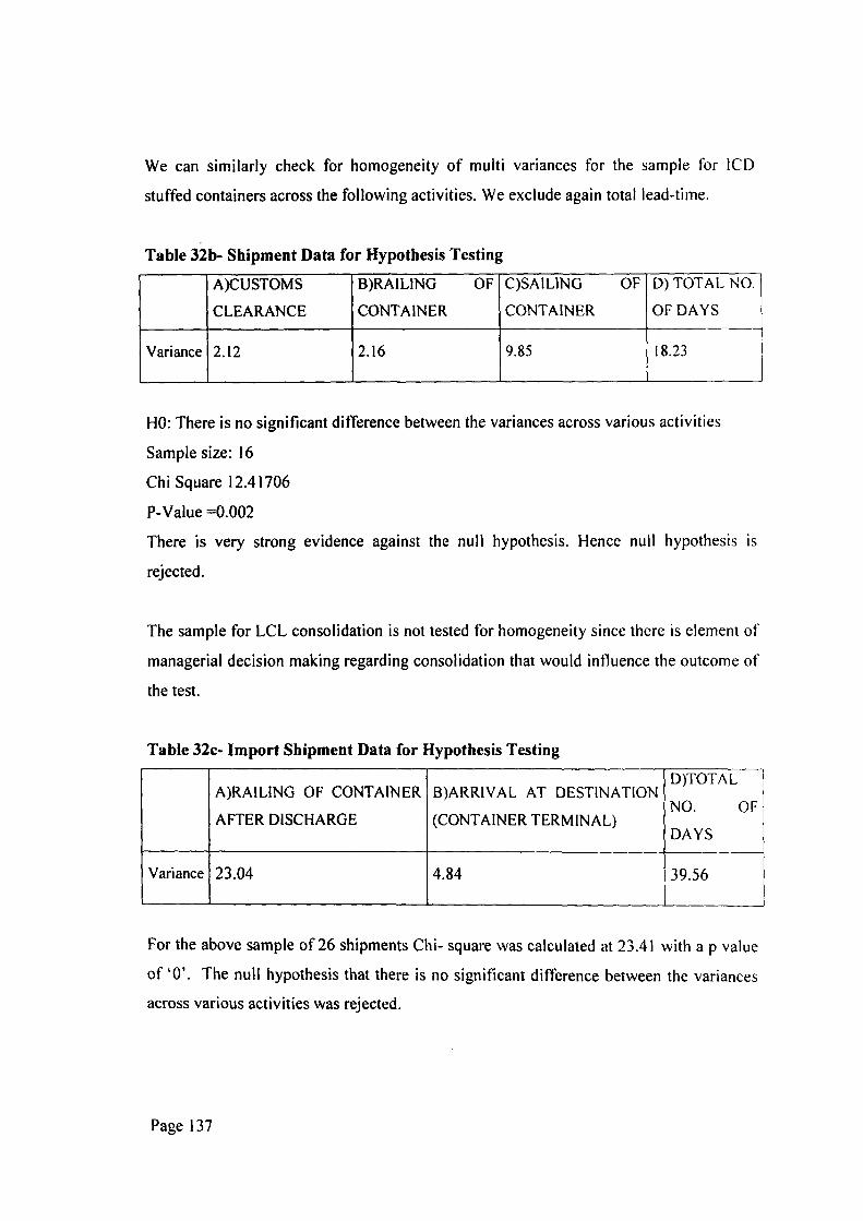
We can similarly check for homogeneity of multi variances for the sample for ICD

stuffed containers across the following activities. We exclude again total lead-time.

Table 32b- Shipment Data for Hypothesis Testing

Variance

AX:USTOMS

CLEARANCE

2.12

B)RA1L1NG OF

CONTAINER

2.16

<

OSAILING OF

CONTAINER

9.85

D) TOTAL NO.

OF DAYS

18.23

HO: There is no significant difference between the variances across various activities

Sample size: 16

Chi Square 12.41706

P-Value =0.002

There is very strong evidence against the null hypothesis. Hence null hypothesis is

rejected.

The sample for LCL consolidation is not tested for homogeneity since there is element of

managerial decision making regarding consolidation that would influence the outcome of

the test.

Table 32c- Import Shipment Data for Hypothesis Testing

Variance

A)RAIL1NG OF CONTAINER

AFTER DISCHARGE

23.04

B)ARRIVAL AT DESTINATION

(CONTAINER TERMINAL)

4.84

D)TOTAL

NO. OF

DAYS

39.56

For the above sample of 26 shipments Chi- square was calculated at 23.41 with a p value

of '0' . The null hypothesis that there is no significant difference between the variances

across various activities was rejected.

Page 137

6.3.4.1 Reasons for Difference in Variance and implications

Of the above variation in sailing can arise out of factors other than inefficacies of the

system. These could be because of shortfall in freight capacity at the port (Freight Market

Dynamics) or because of poor planning by the exporters. Variance in railing lead-time

and arrival at POD lead time would be primarily because of issues pertaining to physical

infrastructure. Container placement to custom clearance covers the activities from

processing of documents to sealing for stuffed container. These activities constitute the

software of the supply chain. Since the difference in the variance at the different stages is

significant we would need to test the correlation between the activities that form part of

the software for the system with total lead-time.

It can be observed from the samples that variance in lead-time is high in these activities.

It is also observed that the variance in the total transit time is greater than the sum of the

variance of the different stages which are linearly linked. For stages linearly linked the

overall variance should be sum of the constituent variances. It was verified that the

difference was not due to sampling error. This implies that the variance at the different

stages have a cascading effect on the overall variance.

6.3.5 Correlation between Total Lead Time and Time Taken Till Containerisation

We wish to examine the effect of the lead-times, from processing of documents to

containerization, on the total lead time. For this we calculate the Carl Pearson's

coefficient of correlation between the two lead times. From the above sample of 52

shipments the correlation between the lead-time for containerization (Empty container

placement to containerization) and total lead time (from empty container placement to

sailing of vessel) was calculated.

The Carl Pearson's coefficient of correlation was calculated as r=0.34

We wish to test the significance of this coefficient at confidence level of 95 % (K = 0.05).

6.3.5.1 Hypothesis testing for correlation.

Null Hypothesis: The null hypothesis states that there is no significant relationship

between the two variables.

HO: r =0

Page 138

Alternative hypothesis: The alternative hypothesis states that there is a significant

positive correlation between the two variables. HO: r >0

We use the single tailed test to test the above hypothesis.

Degrees of freedom: N-2 i.e. 52- 50 = 50

At K = 0.05 and with 50 degrees of freedom the tabulated value of r for single tailed test

is read from Pearson's table as r = 0.231.

Calculated value of r is 0.34.

Since the calculated value of r is greater than the tabulated value we reject the Null

Hypothesis and accept the alternate hypothesis.

Another way of looking at a correlation coefficient is to estimate the amount of common

variance between the two variables that is accounted for by the relationship. This quantity

(proportion of common variance) is the square of the correlation coefficient.

r squared is O.ll.ln terms of percentage 11% of the variation in the total lead-time can be

explained by the variation in time taken up to customs clearance.

Page 139

chapter 6 analysis of quantitative data and discussion on...

Documents