chapter 5 time, frequency, scale and resolutionusers.isr.ist.utl.pt/~aguiar/notes_chapter5.pdf ·...

Chapter 5

Time, Frequency, Scaleand Resolution

Contents

5.1 Introduction . . . . . . . . . . . . . . . . . . . . . . . 193

5.2 Time and Frequency Localization . . . . . . . . . . 194

5.3 Heisenberg Boxes and the Uncertainly Principle . 197

5.4 Scale and Scaling . . . . . . . . . . . . . . . . . . . . 202

5.5 Resolution, Bandwidth and Degrees of Freedom . 204

5.6 Haar Tiling (Old) . . . . . . . . . . . . . . . . . . . 205

5.7 Case Studies . . . . . . . . . . . . . . . . . . . . . . . 208

Chapter at a Glance . . . . . . . . . . . . . . . . . . . . . . 210

Historical Remarks . . . . . . . . . . . . . . . . . . . . . . . 211

Further Reading . . . . . . . . . . . . . . . . . . . . . . . . . 211

Exercises with Solutions . . . . . . . . . . . . . . . . . . . . 211

Exercises . . . . . . . . . . . . . . . . . . . . . . . . . . . . . 212

5.1 Introduction

Over the next several chapters, we embark on the construction of various bases forsignal analysis and synthesis. To create representations

x =∑

k

αkϕk,

we need ϕk to “fill the space” (completeness), and sometimes for ϕk to be anorthonormal set. However, these properties are not enough for a representation tobe useful. For most applications, the utility of a representation is tied to time,frequency, scale, and resolution properties of the ϕks—the topic of this chapter.

Time and frequency properties are perhaps the most intuitive. Think of a basisfunction as a note on a musical score. It has a given frequency (for example, middle

0Last edit: JK Mar 04 08

193

194 Chapter 5. Time, Frequency, Scale and Resolution

A has the frequency of 440Hz) and start time, and its type ( , , ) indicates itsduration. We can think of the musical score as a time-frequency plane34 and notesas rectangles in that plane with horizontal extent determined by start and end timesand vertical extent related in some way to frequency. Mapping a musical score tothe time-frequency plane is far from the artistic view usually associated with music,but it helps visualize the notion of the time-frequency plane (see Figure 5.1).

Time and frequency views of a signal are inter-

FIGURE 1.2 fig1.2

(a)

(b)

Figure 5.1: Musical scoreas an illustration of a time-frequency plane [65].

twined in several ways. The duality of the Fouriertransform gives a precise sense of interchangeability,since if x(t) has the transform X(ω), X(t) has thetransform 2πx(−ω). More relevant to this chapter,the uncertainty principle determines the trade-offbetween concentration in one domain and spreadin the other; signals concentrated in time will bespread in frequency, and, by duality, signals con-centrated in frequency will be spread in time. Italso bounds the product of spreads in time and fre-quency, with the lower bound reached by Gaussianfunctions. This cornerstone result of Fourier theoryis due to Heisenberg in physics and associated withGabor in signal theory (see Historical Remarks).

Another natural notion for signals is scale. For example, given a portrait ofa person, recognizing that person should not depend on whether they occupy one-tenth or one-half of the image.35 Thus, image recognition should be scale invariant.Signals that are scales of each other are often considered as equivalent. However, thisscale invariance is a purely continuous-time property, since discrete-time sequencescannot be rescaled easily. In particular, while continuous-time rescaling can beundone easily, discrete-time rescaling, such as downsampling by a factor of 2, cannotbe undone in general.

A fourth important notion is that of resolution. Intuitively, a blurred photo-graph does not have the resolution of a sharp one, even when the two prints are ofthe same physical size. Thus, resolution is related to bandwidth of a signal, or, moregenerally, to the number of degrees of freedom per unit time (or space). Clearly,scale and resolution interact, and most notably in discrete time.

5.2 Time and Frequency Localization

Time Spread

Consider a function x(t) or a sequence xn, where t or n is a time index. We nowdiscuss localization of the function or sequence in time. The easiest case is when thesupport of the signal is finite, that is, x(t) is nonzero only in [T1, T2], or, xn is nonzeroonly for N1, N1 + 1, . . . , N2. This is often called compact support. If a function(sequence) is of compact support, then its Fourier transform cannot be of compact

34Note that the frequency axis is logarithmic rather than linear.35This is true within some bounds, which is linked to resolution; see below.

5.2. Time and Frequency Localization 195

support (it can only have isolated zeros). That is, a function (sequence) cannot beperfectly localized in both time and frequency. This fundamental property of theFourier transform is explored in Exercise 5.1 for the DFT.

If not of compact support, a signal might decay rapidly as t or n go to ±∞.Such decay is necessary for working in L2(R) or ℓ2(Z); for example, for finite energy(L2(R)), a function must decay faster than |t|−1/2 for large t (see Chapter 3).

A concise way to describe locality (or lack thereof), is to introduce a spreadingmeasure akin to standard deviation, which requires normalization so that |x(t)|2 canbe interpreted as a probability density function.36 Its mean is then the time centerof the function and its standard deviation is the time spread. Denote the energy ofx(t) by

Ex = ‖x‖2 =

∫ ∞

−∞|x(t)|2 dt.

Then define the time center µt as

µt =1

Ex

∫ ∞

−∞t|x(t)|2 dt, (5.1)

and the time spread ∆t as

∆2t =

1

Ex

∫ ∞

−∞(t− µt)

2|x(t)|2 dt. (5.2)

Example 5.1 (Time spreads). Consider the following signals and their time spreads:

(i) The box function

b(t) =

1, −1/2 < t ≤ 1/2;0, otherwise;

(5.3)

has µt = 0 and ∆2t = 1/12.

(ii) For the sinc function from (1.65),

x(t) =1√π

(t) sincπ =1√π

sin t

t,

|x(t)|2 decays only as 1/|t|2, so ∆2t is infinite.

(iii) The Gaussian function as in (1.69) with γ = (2α/π)1/4 is of unit energy as wehave seen in (1.71). Then, the version centered at t = 0 is of the form:

g(t) =

(2α

π

)1/4

e−αt2 , (5.4)

and has µt = 0 and ∆2t = 1.

36Note that this normalization is precisely the same as restricting attention to unit-energy func-tions.


From the above example, we see that the time spread can vary widely. In particular,it can be unbounded, even for functions which are widely used, like the sinc function.Exercise 5.2 explores functions based on the box function and convolutions thereof.

We restrict our definition of the time spread to continuous-time functions fornow. While it can be extended to sequences, it will not be done here since itsfrequency-domain equivalent (where functions are periodic) is not easily generaliz-able.

Exercise 5.3 explores some of the properties of the time spread ∆t: (a) it isinvariant to time shifts x(t−t0); (b) it is invariant to modulations by an exponentialejω0tx(t); (c) energy-conserving scaling by s, 1/

√sx(t/s), increases ∆t by a factor

s.

Frequency Spread

We now discuss the dual concept to time localization of x(t)—frequency localizationof its DTFT pair X(ω). In terms of localization, the simplest case is when X(ω)is of compact support, or, |X(ω)| = 0 for ω /∈ [−Ω,Ω]. This is the notion ofbandlimitidness used in the sampling theorem in Chapter 4. The time domainfunction has infinite support.

Even if not compactly supported, the Fourier transform can have fast decay,and thus the notion of a frequency spread. Similarly to our discussion of the timespread, we normalize the frequency spread, so as to be able to interpret |X(ω)|2 asa probability density function. Denote the energy of X(ω) by

Eω = ‖x‖2 =

∫ ∞

−∞|X(ω)|2 dω.

The frequency center µω is then

µω =1

2πEω

∫ ∞

−∞ω|X(ω)|2 dω, (5.5)

and the frequency spread ∆ω

∆2ω =

1

2πEω

∫ ∞

−∞(ω − µω)2|X(ω)|2 dω. (5.6)

Because of the 2π-periodicity of the Fourier transform X(ejω), there is no naturaldefinition of ∆2

ω for sequences. Thus, we continue to focus on continuous-timefunctions for now.

Example 5.2. Consider a bandlimited Fourier transform given by

X(ω) =

√s, |ω| < π

s ;0, otherwise.

Then

∆2ω =

1

2π

∫ π/s

−π/s

sω2 dω =π2

3s2.

5.3. Heisenberg Boxes and the Uncertainly Principle 197

Figure 5.2: The time-frequency plane and a Heisenberg box. (a) A time-domain functionx(t). (b) Its Fourier transform magnitude |X(ω)|. (c) A Heisenberg box centered at(µt, µω) and of size (∆t,∆ω).

Figure 5.3: A time and/or frequency shift of a function, simply shifts the Heisenbergbox.

The corresponding time-domain function is a sinc, for which we have seen that ∆2t

is unbounded.

Exercise 5.3 explores some of the properties of the frequency spread ∆ω : (a)it is invariant to time shifts x(t − t0); (b) it is invariant to modulations by anexponential ejω0tx(t) (but not to modulations by a real function such as a cosine);(c) energy-conserving scaling by s, 1/

√sx(t/s), decreases ∆ω by a factor s. This is

exactly the inverse of the effect on the time spread, as is to be expected from thescaling property of the Fourier transform.

5.3 Heisenberg Boxes and the Uncertainly Principle

Given a function x(t) and its Fourier transform X(ω), we have the 4-tuple (µt, ∆t,µω, ∆ω) describing the function’s center in time and frequency (µt, µω) and thefunction’s spread in time and frequency (∆t,∆ω). It is convenient to show this in adiagram, as in Figure 5.2. This gives a conceptual picture, conveying the idea thatthere is a center of mass (µt, µω) and a spread (∆t,∆ω) shown by a rectangularbox with appropriate location and size. The plane on which this is drawn is calledthe time-frequency plane, and the box is usually called a Heisenberg box, or atime-frequency tile.

From our previous discussion on time shifting and complex modulation, weknow that a function y(t) obtained by shift and modulation of x(t),

y(t) = ejω0tx(t− t0), (5.7)

will simply have a Heisenberg box shifted by t0 and ω0, as depicted in Figure 5.3.What about scaling? Consider energy-invariant rescaling by a factor s,

y(t) =1√sx(t

s). (5.8)

Figure 5.4: The effect of scaling as in (5.8) on the associated Heisenberg box. The cases = 2 is shown.


If x(t) has a Heisenberg box specified by (µt,∆t, µω,∆ω), then the box for y(t) isspecified by (sµt, µω/s, s∆t,∆ω/s), as shown in Figure 5.4. The effects of shift,modulation and scaling on the Heisenberg boxes of the resulting functions are sum-marized in Table 5.1.

Function Time center Time spread Freq. center Freq. spread

x(t) µt ∆t µω ∆ω

x(t − t0) µt + t0 ∆t µω ∆ω

ejω0x(t) µt ∆t µω + ω0 ∆ω

1√sx(t

s) s µt s∆t

1

sµω

1

s∆ω

Table 5.1: Effect of shift, modulation and scaling on Heisenberg boxes (µt,∆t, µω,∆ω).

So far, we have considered the effect on Heisenberg boxes of shifting in timeand frequency and rescaling of functions. How about their sizes? The intuition,corroborated by what we saw with scaling, is that one can trade time spread forfrequency spread. Moreover, from Examples 5.1 and 5.2, we know that a functionthat is narrow in one domain will be broad in the other. It is thus intuitive that thesize of the Heisenberg box is lower bounded, so that no function can be arbitrarilynarrow in both time and frequency. While the result is often called the Heisenberguncertainty principle, it has been shown independently by a number of others,including Gabor.

Theorem 5.1 (Uncertainty principle). Given a function x ∈ L2(R), the prod-uct of its squared time and frequency spreads is lower bounded as

∆2t ∆2

ω ≥1

4. (5.9)

The lower bound is attained by Gaussian functions from (1.69):

x(t) = γe−αt2 , α > 0. (5.10)

Proof. We prove the theorem for real functions; see Exercise 5.4 for the complexcase. Without loss of generality, assume that x(t) is centered at t = 0, and thatx(t) has unit energy; otherwise we may shift and scale it appropriately. Since x(t)is real, it is also centered at ω = 0, so µt = µω = 0.

Suppose x(t) has a bounded derivative x′(t); if not, ∆2ω =∞ so the statement

holds trivially. Consider the function t x(t)x′(t) and its integral. Using the Cauchy-Schwarz inequality (1.16), we can write

∣∣∣∣∫ ∞

−∞tx(t)x′(t) dt

∣∣∣∣2

≤∫ ∞

−∞|tx(t)|2 dt

∫ ∞

−∞|x′(t)|2 dt

(a)=

∫ ∞

−∞|tx(t)|2 dt

︸︷︷︸∆2

t

1

2π

∫ ∞

−∞|jωX(ω)|2 dt

︸︷︷︸∆2

ω

= ∆2t ∆

2ω , (5.11)


where (a) follows from Parseval’s relation and the fact that x′(t) has Fourier trans-form jωX(ω). We now simplify the left side:∫ ∞

−∞tx(t)x′(t) dt

(a)=

1

2

∫ ∞

−∞tdx2(τ)

dτdt

(b)=

1

2t x2(t)

∣∣∞−∞−

1

2

∫ ∞

−∞x2(t) dt

︸︷︷︸1

(c)= −1

2,

where (a) follows from (x2(t))′ = 2x′(t)x(t); (b) is due to integration by parts;and (c) holds because x(t) ∈ L2(R) implies that it decays faster than 1/

√|t| for

t → ±∞, and thus limt→±∞ tx2(t) = 0 (see Chapter 3). Substituting this into(5.11) yields (5.9).

To find functions that meet the bound with equality, recall that Cauchy-Schwarz inequality becomes an equality if and only if the two functions are collinear(scalar multiples of each other). In our case this means x′(t) = β t x(t). Functions

satisfying this relation have the form x(t) = γ eβt2/2 = γ e−αt2—the Gaussianfunctions.

The uncertainty principle points to a fundamental limitation in time-frequencyanalysis. If we desire to analyze a signal with a “probing function” to extractinformation about the signal around a location (µt, µω), the probing function isnecessarily blurred. That is, if we desire very precise frequency information aboutthe signal, its time location will be uncertain, and vice versa.

Example 5.3 (Sinusoid plus Dirac impulse). A generic example to illustratethe tension between time and frequency resolution is the analysis of a signal con-taining a Dirac impulse in time and a Dirac impulse in frequency:

x(t) = δ(t− τ) + ejΩt,

with the Fourier transform

X(ω) = e−jωτ + 2πδ(ω − Ω).

Clearly, to locate the Dirac impulse in time or in frequency, one needs to be as sharpas possible in the that particular domain, thus compromising the sharpness in theother domain. We illustrate this with a numerical example which, while simple,conveys this basic, but fundamental, trade-off.

Consider a periodic sequence with period N = 256, containing a complexsinusoidal sequence and a Dirac impulse, as shown in Figure 5.5(a). In Figure 5.5(b),we show the magnitude of the DFT of one period, which has 256 frequency bins, andperfectly identifies the exponential component, while missing the time-domain Diracimpulse completely. In order to increase the time resolution, we divide the periodinto 16 pieces of length 16, taking the DFT of each, as shown in Figure 5.5(c). Now,we can identify approximately where the time-domain Dirac impulse occurs, but inturn, the frequency resolution is reduced, since we now have only 16 frequency bins.Finally, Figure 5.5(d) shows the dual case to Figure 5.5(b), that is, we plot themagnitude of each sample over time. The Dirac impulse is now perfectly visible,while the sinusoid is just a background wave, with its frequency not easily identified.


Figure 5.5: Time-frequency resolution trade-off for a signal containing a Dirac impulsein time and a complex sinusoid (Dirac impulse in frequency). (a) Original signal of length256. (b) Magnitude of discrete-time Fourier transform. (c) Same as (b), but with signalsplit into 16 pieces of length 16 each. (d) Magnitude of samples.

Example 5.4 (Chirp signal). As another example of time-frequency analysis andthe trade-off between time and frequency sharpness, we consider a signal consistingof a windowed chirp (complex exponential with a rising frequency). Instead of afixed frequency ω0, the “local frequency” is linearly growing with time: ω0t. Thesignal is

x(t) = w(t) ejω0t2 ,

where w(t) is an appropriate window function. Such a chirp signal is not as esotericas it may look; bats use such signals to hunt for bugs. An example is given inFigure 5.6(a), and an “ideal” time-frequency analysis is sketched in Figure 5.6(b).

As analyzing functions, we choose windowed complex exponentials (but witha fixed frequency). The choice we have is the size of the window (assuming the an-alyzing function will cover all shifts and modulations of interest). A short windowallows for sharp frequency analysis, however, no frequency is really present otherthan at one instant! A short window will do justice to the transient nature of “fre-quency” in the chirp, but will only give a very approximate frequency analysis dueto the uncertainty principle. A compromise between time and frequency sharpnessmust be sought, and one such possible analysis is shown in Figure 5.7.

While the uncertainty principle uses a spreading measure akin to variance,other measures can be defined. Though they typically lack fundamental bounds ofthe kind given by the uncertainty principle (5.9), they can be quite useful as well asintuitive. One such measure, easily applicable to functions that are symmetric inboth time and frequency, finds the centered intervals containing α% of the energyin time and frequency (where α is typically 90 or 95). For a function x(t) of unit

norm and symmetric around µt, the time spread ∆(α)t is now defined such that

∫ µt+12

b∆(α)t

µt− 12

b∆(α)t

|x(t)|2 dt = α. (5.12)

Similarly, the frequency spread ∆(α)ω around the point of symmetry µω is defined

such that

1

2π

∫ µω+12

b∆(α)ω

µω− 12

b∆(α)ω

|X(ω)|2 dω = α. (5.13)

Exercise 5.3(c) shows that ∆(α)t and ∆

(α)ω satisfy the same shift, modulation and

scaling behavior as ∆t and ∆ω in Table 5.1.


Figure 5.6: Chirp signal and time-frequency analysis with a linearly increasing frequency.(a) An example of a windowed chirp with a linearly increasing frequency. Real and imag-inary parts are shown as well as the raised cosine window. (b) Idealized time-frequencyanalysis.

Figure 5.7: Analysis of a chirp signal. (a) One of the analyzing functions, consisting ofa (complex) modulated window. (b) Magnitude squared of the inner products betweenthe chirp and various shifts and modulates of the analyzing functions, showing a blurredversion of the chirp.

Uncertainty Principle for Discrete Time

Thus far, we have restricted our attention to (continuous-time) functions. Analo-gous results for (discrete-time) sequences are not as elegant, except in the case ofstrictly lowpass sequences.

For x ∈ ℓ2(Z) with energy Ex =∑

n |xn|2, define the time center µn and timespread ∆n as

µn =1

Ex

∑

n∈Z

n |xn|2 and ∆2n =

1

Ex

∑

n∈Z

(n− µn)2|xn|2.

Define the frequency center µω and frequency spread ∆ω as

µω =1

2πEx

∫ π

−π

ω|X(ejω)|2 dω and ∆2ω =

1

2πEx

∫ π

−π

(ω − µω)2|X(ejω)|2 dω.

Because of the interval of integration [−π, π], the value of µω may not match theintuitive notion of frequency center of the sequence. For example, while a sequencesupported in Fourier domain on ∪k∈Z [0.9π + k2π, 1.1π + k2π] seems to have itsfrequency center near π, µω may be far from π. (TBD: Expand)

With these definitions paralleling those for continuous-time functions, we canobtain a result very similar to Theorem 5.1. One could imagine that it follows fromcombining Theorem 5.1 with Nyquist-rate sampling of a bandlimited function. Theproof suggested in Exercise 5.5 uses the Cauchy-Schwarz inequality similarly to ourearlier proof.

Theorem 5.2 (Discrete-time uncertainty principle). Given a sequence x ∈ℓ2(Z) with X(ejπ) = 0, the product of its squared time and frequency spreads islower bounded as

∆2n ∆2

ω >1

4. (5.14)

In addition to the above uncertainty principle for infinite sequences, there is a simpleand powerful uncertainty principle for finite-dimensional sequences and their DFTs.This is explored in Exercise 5.8 and arises again in Chapter (TBD).


n

xn

n

yn

n

zn

(a) (b) (c)

Figure 5.8: Stretching of a sequence by a factor 2, followed by contraction. This isachieved with upsampling by 2, followed by downsampling by 2, recovering the original.(a) Original. (b) Upsampled. (c) Downsampled.

5.4 Scale and Scaling

In the previous section, we introduced the idea of signal analysis as computing aninner product with a “probing function.” Along with the Heisenberg box 4-tuple,another key property of a probing function is its scale. Scale is closely related totime spread, but it is inherently a relative (rather than absolute) quantity. Beforefurther describing scale, let us revisit scaling, especially to point out the fundamentaldifference between continuous- and discrete-time scaling operations.

An energy-conserving rescaling of x(t) by a factor s ∈ R+ yields

y(t) =√s x(st)

FT←→ Y (ω) =1√sX(

ω

s). (5.15)

Clearly, such continuous-time scaling is reversible, since a rescaling of y(t) by (1/s)gives

1√sy(t

s) = x(t).

The situation is more complicated in discrete time, where we need multiratesignal processing tools introduced in Section 2.5. Given a sequence xn, a “stretch-ing” by an integer factor N can be achieved by upsampling by N as in (2.129). Thiscan be undone by downsampling by N as in (2.121) (see Figure 5.8).

If instead of stretching, we want to “contract” a sequence by an integer factorN , we can do this by downsampling by N . However, such an operation cannot beundone, as (N − 1) samples out of every N have been lost, and are replaced byzeros during upsampling (see an example for N = 2 in Figure 5.9).

Thus, scale changes are more complicated in discrete time. In particular,compressing the time axis cannot be undone since samples are lost in the opera-tion. Scale changes by rational factors are possible through combinations of integerupsampling and downsampling, but cannot be undone in general (see Exercise 5.6).

Let us go back to the notion of scale, and think of a familiar case where scaleplays a key role—maps. The usual notion of scale in maps is the following: a mapof scale 1:100,000 is a representation where an object of length 1 km is representedby a length of (103m)/105 = 1cm. That is, the scale factor s = 105 is used as

5.4. Scale and Scaling 203

n

xn

n

yn

n

zn

(a) (b) (c)

Figure 5.9: Contraction of a sequence by a factor 2, followed by stretching, using down-sampling and upsampling. The result equals the original only at even indices, z2n = x2n,and is zero elsewhere. (a) Original sequence x. (b) Downsampled sequence y. (c) Upsam-pled sequence z.

Figure 5.10: Aerial photographs of the EPF Lausanne campus at various scales. (a)5,000. (b) 10,000. (c) 20,000.

a contraction factor, to map a reality x(t) into a scaled version y(t) =√sx(st)

with the energy normalization factor√s of no realistic significance because reality

and a map are not of the same dimension. However, reality does provide us withsomething important: a baseline scale against which to compare the map.

When we look at functions in L2(R), a baseline scale does not necessarilyexist. When y(t) =

√sx(st), we say that y is at a larger scale if s > 1, and at

a smaller scale if s ∈ (0, 1). There is no absolute scale for y unless we arbitrarilydefine a scale for x. We indeed do this sometimes, as we will see in Chapter (TBD).

Now consider the use of a probing function ϕ(t) to extract some informationabout x(t). If we compute the inner product between the probing function and ascaled function, we get

⟨√sx(st), ϕ(t)

⟩=√s

∫x(st)ϕ(t) dt =

1√s

∫x(τ)ϕ(

τ

s) dτ

=

⟨x(t),

1√sϕ(t/s)

⟩. (5.16)

Probing a contracted function is equivalent to stretching the probe, thus emphasiz-ing that scale is relative. If only stretched and contracted versions of a single probeare available, large scale features in x(t) are seen using stretched probing functions,while fine details in x(t) are seen using contracted probing functions.

In summary, large scales s ≫ 1 correspond to contracted versions of reality,or to widely spread probing functions. This duality is inherent in the inner product(5.16). Figure 5.10 shows an aerial photograph with different scale factors as perour convention, while Figure 5.11 shows the interaction of signals with various sizefeatures and probing functions.


Figure 5.11: Signals with features at different scales require probing functions adaptedto the scales of those features. (a) A wide-area feature requires a wide probing function.(b) A sharp feature requires a sharp probing function.

5.5 Resolution, Bandwidth and Degrees of Freedom

The notion of resolution is intuitive for images. If we compare two photographs ofthe same size depicting the same reality, one sharp and the other blurry, we saythat the former has higher resolution than the latter. While this intuition is relatedto a notion of bandwidth, it is not the only interpretation.

A more universal notion is to define resolution as the number of degrees offreedom per unit time (or unit space for images) for a set of signals. Classicalbandwidth is then proportional to resolution. Consider the set of functions x(t)with spectra X(ω supported on the interval [−Ω,Ω]. Then, the sampling theorem(see Chapter 4) states that samples taken every T = π/Ωsec, or xn = x(nT ), n ∈ Z,uniquely specify x(t). In other words, real functions of bandwidth 2Ω have Ω/π realdegrees of freedom per unit time.

As an example of a set of functions that, while not bandlimited, do havea finite number of degrees of freedom per unit time, consider piecewise constantfunctions over unit intervals:

x(t) = x⌊t⌋ = xn, n ≤ t < n+ 1, n ∈ Z. (5.17)

Clearly, x(t) has 1 degree of freedom per unit time, but an unbounded spectrumsince it is discontinuous at every integer. This function is part of a general class offunctions belonging to the so-called shift-invariant subspaces we studied in Chap-ter 4 (see also Exercise 5.7).

Scaling affects resolution, and as in the previous section there is a differencebetween discrete and continuous time. For sequences, we start with a referencesequence space S in which there are no fixed relationships between samples and therate of the samples is taken to be 1 per unit time. In the reference space, the resolu-tion is 1 per unit time because each sample is a degree of freedom. Downsampling asequence from S by N leads to a sequence having a resolution of 1/N per unit time.Higher-resolution sequences can be obtained by combining sequences appropriately;see Example 5.5 below. For continuous-time functions, scaling is less disruptive tothe time axis, so calculating the number of degrees of freedom per unit time is notdifficult. If x(t) has resolution τ (per unit time), then x(αt) has resolution ατ .

Filtering can affect resolution as well. If a function of bandwidth [−Ω,Ω] isperfectly lowpass filtered to [−βΩ, βΩ], 0 < β < 1, then its resolution changes fromΩ/π to βΩ/π. The same holds for sequences, where an ideal lowpass filter withsupport [−βπ, βπ], 0 < β < 1, reduces the resolution to β samples per unit time.

Example 5.5 (Scale and resolution). First consider the continuous-time case.Let x(t) be a bandlimited function with frequency support [−Ω,Ω]. Then y(t) =√

2x(2t) has doubled scale and resolution. Inversely, y(t) = 1√2x(t/2) has half the

5.6. Haar Tiling (Old) 205

Figure 5.12: Interplay of scale and resolution for continuous- and discrete-time signals.We assume the original signal to have scale s = 1 and resolution τ = 1, and indicatethe resulting scale and resolution of the output by s′ and τ ′. (a) Filtering of signal. (b)Downsampling by 2. (c) Upsampling by 2. (d) Downsampling followed by upsampling.(e) Filtering and downsampling. (f) Upsampling and filtering.

scale and half the resolution. Finally, y(t) = (h ∗ x) (t), where h(t) is an ideal low-pass filter with support [−Ω/2,Ω/2], has unchanged scale but half the resolution.

Now let xn be a discrete-time sequence. The downsampled sequence yn as in(2.116) has doubled scale and half the resolution with respect to xn. The upsampledsequence yn as in (2.117) has half the scale and unchanged resolution. A sequencefirst downsampled by 2 and then upsampled by 2 keeps all the even samples andzeros out the odd ones, with unchanged scale and half the resolution. Finally,filtering with an ideal halfband lowpass filter with frequency support [−π/2, π/2]leaves the scale unchanged, but halves the resolution. Some of the above relationsare depicted in Figure 5.12.

5.6 Haar Tiling (Old)

(b) (c)

(a)

xn xv

n

xn xv

22g n– gn

n

Figure 5.13: Smoothing operator. (a) Block diagram. (b) An example signal. (c)Smoothed signal from part (b).

Example 5.6 (How does Haar tile the time-frequency plane?). To illus-trate the concepts introduced in this chapter and to give a hint of where we aregoing, we go back to our favorite example—Haar. Recall the smoothing and differ-encing operators we covered in Section ??. We want to try to get a slightly betterfrequency localization than that obtained by the Dirac representation. Thus, weuse the Haar filters and first smooth our signal. This is shown in Fig. 5.13. We


(b) (c)

(a)

xn xw

n

xn xw

22h n– hn

n

Figure 5.14: Differencing operator. (a) Block diagram. (b) An example signal. (c)Differenced signal from part (b).

(b)

(a)

xn

x=xV+xW

22h n– hn

22g n– gn

xn+

n

n

n

xw

xV

xV

xw

Figure 5.15: Putting it all together. The two-channel filter bank implementing bothprojections onto the smooth space as well as the detail space, the sum of which gives backthe original signal.

5.6. Haar Tiling (Old) 207

gn gn 6–gn 4–gn 2–

hn hn 6–hn 4–hn 2–

n

ωπ

π /2

2 4 6 8

Figure 5.16: Time-frequency tiling obtained with the Haar basis.

know that

gn =1√2(δn + δn−1),

and 〈g·, g·−2k〉 = δk. We also know that this combination is an orthogonal projection

PV1 = GU2D2GT

onto the space of smooth signals we call V1. Recall from before ((??)-(??)) that abasis for that space is Φg = g·−2kk∈Z. You can see in Fig. 5.13(b) an example ofthe original signal while in part (c) we see the result of applying operator PV1 to it,that is,

xV1 =[. . . 1

2 (x0 + x1)12 (x0 + x1)

12 (x2 + x3)

12 (x2 + x3) . . .

].

We can now repeat the process for the differencing operator, shown in Fig. 5.14.Now

hn =1√2(δn − δn−1),

and 〈h·, h·−2k〉 = δk. We know that this combination is an orthogonal projectionas well,

PW1 = HU2D2HT ,

onto the space of detail signals we call W1. A basis for that space is Φh =h·−2kk∈Z. You can see in Fig. 5.14(b) an example of the original signal whilein part (c) we see the result of applying operator PW1 to it, that is,

xW1 =[. . . 1

2 (x0 − x1) − 12 (x0 − x1)

12 (x2 − x3) − 1

2 (x2 − x3) . . .].

If we look carefully at parts (c) of Figs. 5.13 and 5.14, we see that the originalsignal can be obtained by summing the two. This is shown in Fig. 5.15. One canverify then that a basis for the original space is Φ = g·−2k, h·−2kk∈Z. The originalsignal is the sum of the two projections:

x = xV1 + xW1 = PV1x+ PW1x,


implemented by a two-channel filter bank given in Fig. 5.15(a). Finally, such adecomposition has an associated time-frequency tiling given in Fig. 5.16. Each tilecorresponds to one basis function. What we can see is exactly what we expected:The frequency localization of the Haar basis is better than that of the Dirac rep-resentation as the frequency has been split in half; the price we paid was a slightlyworse time localization as shown by the basis functions now being of length 2.

Can we do better than that? As a preview of coming attractions, considersmoothing the smoothed version some more. What do we get? We start gettingbetter frequency localization at low frequencies while keeping good time localizationat high frequencies (see Fig. 5.17). To see what the basis is now, we need totransform this filter bank into an equivalent three-channel filter bank as in Fig. 5.18.To do that, we need to use the identities on how we can interchange filtering andsampling given in Section ??. We write expressions for equivalent filters in z-transform-domain:

H(1)(z) = H(z) =1√2(1− z−1),

H(2)(z) = G(z)H(z2) =1

2(1 + z−1 − z−2 − z−3),

G(2)(z) = G(z)G(z2) =1

2(1 + z−1 + z−2 + z−3),

giving rise to the following output signals:

xW1 =[. . . 1

2 (x0 − x1) − 12 (x0 − x1)

12 (x2 − x3) − 1

2 (x2 − x3) . . .],

xW2 =[. . . 1

4 (x0 + x1 − x2 − x3)14 (x0 + x1 − x2 − x3)

− 14 (x0 + x1 − x2 − x3) − 1

4 (x0 + x1 − x2 − x3) . . .],

xV2 =[. . . 1

4 (x0 + x1 + x2 + x3)14 (x0 + x1 + x2 + x3)

14 (x0 + x1 + x2 + x3)

14 (x0 + x1 + x2 + x3) . . .

].

It is easy to see that summing these three signals, we get the original signal back.Continuing in this way, we will get to the discrete wavelet transform with Haarfilters. Fig. 5.19 shows the associated time-frequency tiling.

Fig. 5.20 shows some possibilities of tiling the time-frequency plane and varioustrade-offs involved. Part (a) is the DWT with 3 levels, in part (b) we kept onsplitting the highpass channel, while part (c) shows a more arbitrary tiling.

5.7 Case Studies

So far, our discussion has been mostly conceptual, and the examples synthetic.We now look at case studies using real-world signals such as music, images andcommunication signals. Our discussion is meant to develop intuition rather than berigorous. We want to excite you to continue studying the rich set of tools responsiblefor examples below.

5.7. Case Studies 209

5.7.1 Music and Time-Frequency Analysis

5.7.2 Images and Pyramids

5.7.3 Singularities, Denoising and Superresolution

5.7.4 Channel Equalization and OFDM


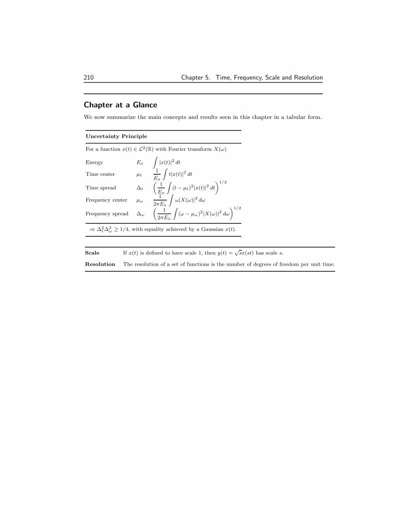
Chapter at a Glance

We now summarize the main concepts and results seen in this chapter in a tabular form.

Uncertainty Principle

For a function x(t) ∈ L2(R) with Fourier transform X(ω)

Energy Ex

Z|x(t)|2 dt

Time center µt1

Ex

Zt|x(t)|2 dt

Time spread ∆t

„1

Ex

Z(t− µt)

2|x(t)|2 dt«1/2

Frequency center µω1

2πEx

Zω|X(ω)|2 dω

Frequency spread ∆ω

„1

2πEx

Z(ω − µω)2|X(ω)|2 dω

«1/2

⇒ ∆2t ∆2

ω ≥ 1/4, with equality achieved by a Gaussian x(t).

Scale If x(t) is defined to have scale 1, then y(t) =√sx(st) has scale s.

Resolution The resolution of a set of functions is the number of degrees of freedom per unit time.

Historical Remarks 211

Historical Remarks

Uncertainty principles stemming from the Cauchy-Schwarz in-equality have a long and rich history. The best known one isHeisenberg’s uncertainty principle in quantum physics, first de-veloped in a 1927 essay [31]. Werner Karl Heisenberg (1901-1976) was a German physicist, credited as a founder of quantummechanics, for which he was awarded the Nobel Prize in 1932. Hehad seven children, one of whom, Martin Heisenberg, was a cel-ebrated geneticist. He collaborated with Bohr, Pauli and Dirac,among others. While he was initially attacked by the Nazi warmachine for promoting Einstein’s views, he did head the Nazi

nuclear project during the war. His role in the project has been a subject of controversyevery since, with differing views on whether he was deliberately stalling Hitler’s efforts ornot.

Kennard is credited with the first mathematically exact formula-

tion of the uncertainty principle, and Robertson and Schrodinger

provided generalizations. The uncertainty principle presented in

Theorem 5.1 was proven by Weyl and Pauli and introduced to sig-

nal processing by Dennis Gabor (1900-1979) [25], a Hungar-

ian physicist, and another winner of the Nobel Prize for physics

(he is also known as inventor of holography). By finding a lower

bound to ∆t∆ω, Gabor was intending to define an information

measure or capacity for signals. Shannon’s communication the-

ory [52] proved much more fruitful for this purpose, but Gabor’s

proposal of signal analysis by shifted and modulated Gaussian

functions has been a cornerstone of time-frequency analysis ever

since. Slepian’s survey [53] is enlightening on these topics.

Further Reading

Many of the uncertainty principles for discrete-time signals are considerably more com-plicated than Theorem 5.2. We have given only a result that follows papers by Ishii andFurukawa [34] and Calvez and Vilbe [7].

Donoho and Stark [20] derived new uncertainty principles in various domains. Partic-

ularly influential was an uncertainty principle for finite-dimensional signals and a demon-

stration of its significance for signal recovery (see Exercises 5.8 and 5.9). More recently,

Donoho and Huo [19] introduced performance guarantees for ℓ1 minimization-based signal

recovery algorithms; this has sparked a large body of work.

Exercises with Solutions

5.1. TBD


Exercises

5.1. Finite Sequences and Their DFTs:

Show that if a sequence has a finite number of terms, then its DFT cannot be zero overan interval (that is, it can only have isolated zeros). Conversely, show that if a discreteFourier transform is zero over an interval, then the corresponding sequence has an infinitenumber of nonzero terms.

5.2. Box Function, Its Convolution, and Limits:

Given is the box function from (5.3).

(i) What is the time spread ∆2t of the triangle function (b ∗ b)?

(ii) What is the time spread ∆2t of the function b convolved with itself N times?

5.3. Properties of Time and Frequency Spreads:

Consider the time and frequency spreads as defined in (5.2) and (5.6), respectively.

(i) Show that time shifts and complex modulations of x(t) as in (5.7) leave ∆t and ∆ω

unchanged.

(ii) Show that energy conserving scaling of x(t) as in (5.8) increases ∆t by s, whiledecreasing ∆ω by s, thus leaving the time-frequency product unchanged.

(iii) Show (i)-(ii) for the time-frequency spreads ∆(α)t and ∆

(α)ω as defined in (5.12) and

(5.13).

5.4. Uncertainty Principle for Complex Functions:

Prove Theorem 5.1 without assuming that x(t) is a real function.(Hint: The proof requires more than the Cauchy-Schwarz inequality and integration byparts. Use the product rule of differentiation, d

dt|x(t)|2 = x′(t)x∗(t)+x′∗(t)x(t). Also, use

that for any α ∈ C, |α| ≥ 12|α+ α∗|.)

5.5. Discrete-Time Uncertainty Principle:

Prove Theorem 5.2 for real sequences. Do not forget to provide an argument for thestrictness of inequality (5.14).

(Hint: Use the Cauchy-Schwarz inequality to bound

˛˛Z π

−πωX(ejω)

hd

dωX(ejω)

idω

˛˛2

).

5.6. Rational Scale Changes on Sequences:

A scale change by a factor M/N can be achieved by upsampling by M followed by down-sampling by N .

(i) Consider a scale change by 3/2, and show that it can be implemented either byupsampling by 3, followed by downsampling by 2, or the converse.

(ii) Show that the scale change by 3/2 cannot be undone, even though it is a stretchingoperation.

(iii) Using the fact that whenM and N are coprime, upsampling byM and downsamplingby N commute, show that a sampling rate change by M/N cannot be undone unlessN = 1.

5.7. Shift-Invariant Subspaces and Degrees of Freedom:

Define a shift-invariant subspace S as

S = span(ϕ(t − nT )n∈Z), T ∈ R+.

(i) Show that the piecewise-constant function defined in (5.17) belongs to such a spacewhen ϕ(t) is the indicator function of the interval [0, 1] and T = 1.

(ii) Show that a function in S has exactly 1/T degrees of freedom per unit time.

5.8. Uncertainty Principle for the DFT:

Let x and X be a length-N DFT pair, and let Nt and Nω denote the number of nonzerocomponents of x and X, respectively.

Exercises 213

(i) Prove that X cannot have Nt consecutive zeros, where “consecutive” is interpretedmodN .(Hint: For an arbitrary selection of Nt consecutive components of X, form a linearsystem relating the nonzero components of x to the selected components of X.)

(ii) Using the result of the first part, prove NtNω ≥ N . This uncertainty principle isdue to Donoho and Stark [20].

5.9. Signal Recovery Based on the Finite-Dimensional Uncertainty Principle:

Suppose the DFT of a length-N signal x is known to have onlyNω nonzero components. Us-ing the result of Exercise 5.8, show that the limited DFT-domain support makes it possibleto uniquely recover x from any M (time-domain) components as long as 2(N−M)Nω < N .(Hint: Show that nonunique recovery leads to a contradiction.)


(b)

(a)

n

x=xV +xW+xW

22h n– hn

22g n– gn

x+

n

n

n

xw

xV

xV

xw

22h n– hn

22g n– gn

+

xw

xV

1

1

2

2

x=xV +xW

n

n

nxV

xw

n

xw

1

2

1

1

1

1 1

2

2 2 1

Figure 5.17: What worked once works again; We smooth the already smoothed versionof the signal some more.

Exercises 215

xn

22h n– hn

44h n– hnxn+

xW

xW2

1

44g n– gn xV2

(1)

(2)

(2)

(1)

(2)

(2)

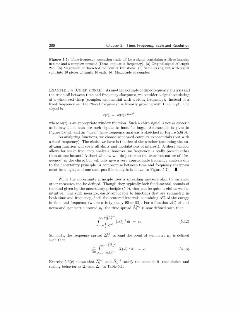
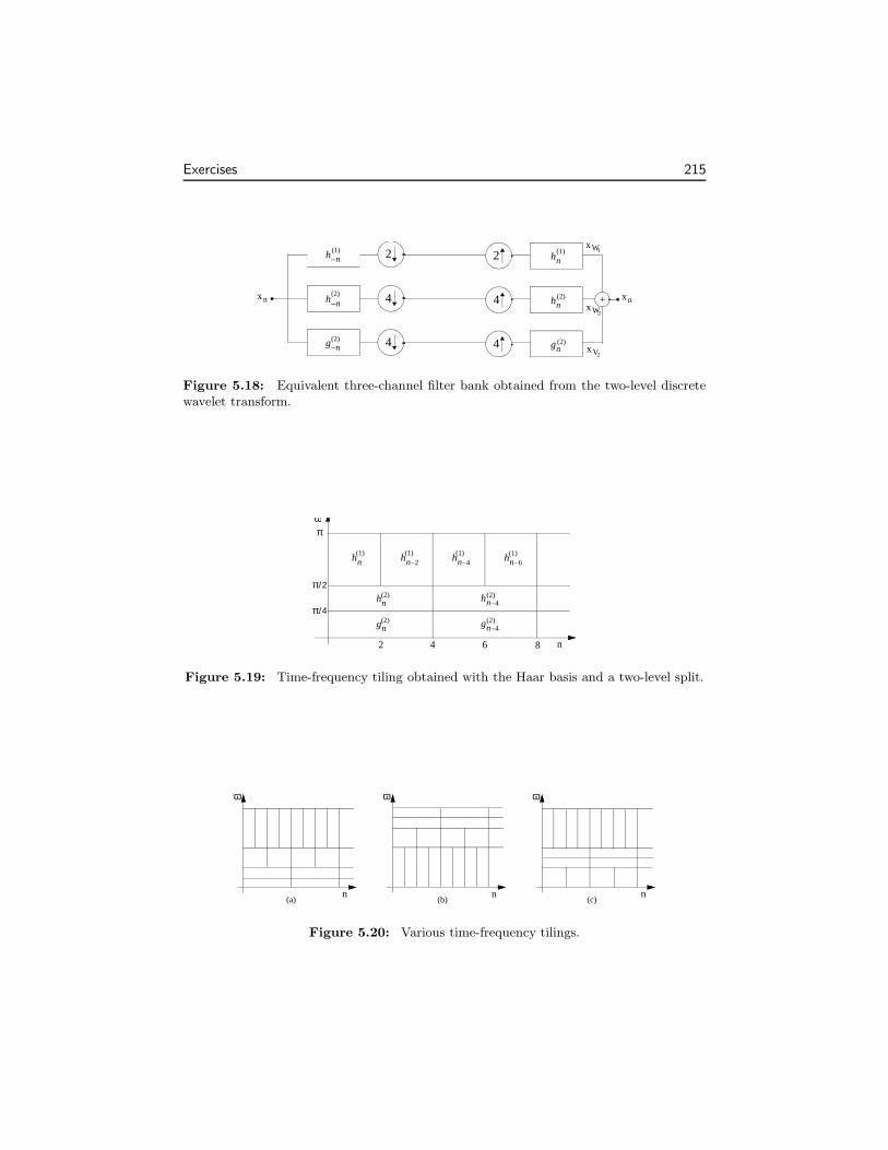
Figure 5.18: Equivalent three-channel filter bank obtained from the two-level discretewavelet transform.

hn hn 6–hn 4–hn 2–

n

ωπ

π /2

2 4 6 8

hn hn 4–(2)(2)

(1) (1) (1) (1)

gn gn 4–(2)(2)

π /4

Figure 5.19: Time-frequency tiling obtained with the Haar basis and a two-level split.

n

ω

n

ω

n

ω

(a) (b) (c)

Figure 5.20: Various time-frequency tilings.

chapter 5 time, frequency, scale and resolutionusers.isr.ist.utl.pt/~aguiar/notes_chapter5.pdf ·...

Documents