chapter 5: the generalized linear regression model and ... · 2. the generalized linear regression...
TRANSCRIPT
Chapter 5: The Generalized Linear Regression Modeland Heteroscedasticity
Advanced Econometrics - HEC Lausanne
Christophe Hurlin
University of Orléans
December 15, 2013
Christophe Hurlin (University of Orléans) Advanced Econometrics - HEC Lausanne December 15, 2013 1 / 153

Section 1
Introduction
Christophe Hurlin (University of Orléans) Advanced Econometrics - HEC Lausanne December 15, 2013 2 / 153

1. Introduction
The outline of this chapter is the following:
Section 2. The generalized linear regression model
Section 3. Ine¢ ciency of the Ordinary Least Squares
Section 4. Generalized Least Squares (GLS)
Section 5. Heteroscedasticity
Section 6. Testing for heteroscedasticity
Christophe Hurlin (University of Orléans) Advanced Econometrics - HEC Lausanne December 15, 2013 3 / 153

1. Introduction
References
Amemiya T. (1985), Advanced Econometrics. Harvard University Press.
Greene W. (2007), Econometric Analysis, sixth edition, Pearson - PrenticeHil (recommended)
Pelgrin, F. (2010), Lecture notes Advanced Econometrics, HEC Lausanne (aspecial thank)
Ruud P., (2000) An introduction to Classical Econometric Theory, OxfordUniversity Press.
Christophe Hurlin (University of Orléans) Advanced Econometrics - HEC Lausanne December 15, 2013 4 / 153

1. Introduction
Notations: In this chapter, I will (try to...) follow some conventions ofnotation.
fY (y) probability density or mass function
FY (y) cumulative distribution function
Pr () probability
y vector
Y matrix
Be careful: in this chapter, I dont distinguish between a random vector(matrix) and a vector (matrix) of deterministic elements (except in section2). For more appropriate notations, see:
Abadir and Magnus (2002), Notation in econometrics: a proposal for astandard, Econometrics Journal.
Christophe Hurlin (University of Orléans) Advanced Econometrics - HEC Lausanne December 15, 2013 5 / 153

Section 2
The generalized linear regression model
Christophe Hurlin (University of Orléans) Advanced Econometrics - HEC Lausanne December 15, 2013 6 / 153

2. The generalized linear regression model
Objectives
The objective of this section are the following:
1 Dene the generalized linear regression model
2 Dene the concept of heteroscedasticity
3 Dene the concept of autocorrelation (or correlation) of disturbances
Christophe Hurlin (University of Orléans) Advanced Econometrics - HEC Lausanne December 15, 2013 7 / 153

2. The generalized linear regression model
Consider the (population) multiple linear regression model:
y = Xβ+ ε
where (cf. chapter 3):
y is a N 1 vector of observations yi for i = 1, ..,N
X is a N K matrix of K explicative variables xik for k = 1, .,K andi = 1, ..,N
ε is a N 1 vector of error terms εi .
β = (β1..βK )> is a K 1 vector of parameters
Christophe Hurlin (University of Orléans) Advanced Econometrics - HEC Lausanne December 15, 2013 8 / 153

2. The generalized linear regression model
In chapter 3 (linear regression model), we assume spherical disturbances(assumption A4):
V (εjX) = σ2IN
In this chapter, we will relax the assumption that the errors areindependent and/or identically distributed and we will study:
1 Heteroscedasticity
2 Autocorrelation or correlation.
Christophe Hurlin (University of Orléans) Advanced Econometrics - HEC Lausanne December 15, 2013 9 / 153

2. The generalized linear regression model
Denition (Generalized linear regression model)The generalized linear regression model is dened as to be:
y = Xβ+ ε
where X is a matrix of xed or random regressors, β 2 RK , and the errorterm ε satises:
E (εjX) = 0N1V (εjX) = Σ = σ2Ω
where Ω and Σ are symmetric positive denite matrices.
Christophe Hurlin (University of Orléans) Advanced Econometrics - HEC Lausanne December 15, 2013 10 / 153

2. The generalized linear regression model
Reminder
V (εjX)| z NN
= E
εε>X| z
NN
=
0BB@V
ε21X Cov ( ε1ε2jX) .. Cov ( ε1εN jX)
E ( ε2ε1jX) V
ε22X .. Cov ( ε2εN jX)
.. .. .. ..Cov ( εN ε1jX) .. .. V
ε2NX
1CCA
Christophe Hurlin (University of Orléans) Advanced Econometrics - HEC Lausanne December 15, 2013 11 / 153

2. The generalized linear regression model
Remark
In the generalized linear regression model, we have
V (εjX) = Σ = σ2Ω
with
Σ =
0BB@σ21 σ12 .. σ1Nσ21 σ22 .. σ2N.. .. .. ..
σN1 .. .. σ2N
1CCA = σ2
0BB@ω11 ω12 .. ω1N
ω21 ω22 .. ω2N
.. .. .. ..ωN1 .. .. ωNN
1CCAand ωij = σij/σ2.
Christophe Hurlin (University of Orléans) Advanced Econometrics - HEC Lausanne December 15, 2013 12 / 153

2. The generalized linear regression model
Denition (Heteroscedasticity)
Disturbances are heteroscedastic when they have di¤erent (conditional)variances:
V ( εi jX) 6= V ( εj jX) for i 6= j
Christophe Hurlin (University of Orléans) Advanced Econometrics - HEC Lausanne December 15, 2013 13 / 153

2. The generalized linear regression model
Remarks
1 Heteroscedasticity often arises in volatile high-frequency time-seriesdata such as daily observations in nancial markets.
2 Heteroscedasticity often arises in cross-section data where the scaleof the dependent variable and the explanatory power of the modeltend to vary across observations. Microeconomic data such asexpenditure surveys are typical
Christophe Hurlin (University of Orléans) Advanced Econometrics - HEC Lausanne December 15, 2013 14 / 153

2. The generalized linear regression model
Example (Heteroscedasticity)If the disturbances are heteroscedastic but they are still assumed to beuncorrelated across observations, so Ω and Σ would be:
Σ =
0BB@σ21 0 .. 00 σ22 .. 0.. .. .. ..0 .. .. σ2N
1CCA = σ2Ω = σ2
0BB@ω1 0 .. 00 ω2 .. 0.. .. .. ..0 .. .. ωN
1CCAwith ωi = σ2i /σ2 for i = 1, ..,N.
Christophe Hurlin (University of Orléans) Advanced Econometrics - HEC Lausanne December 15, 2013 15 / 153
2. The generalized linear regression model
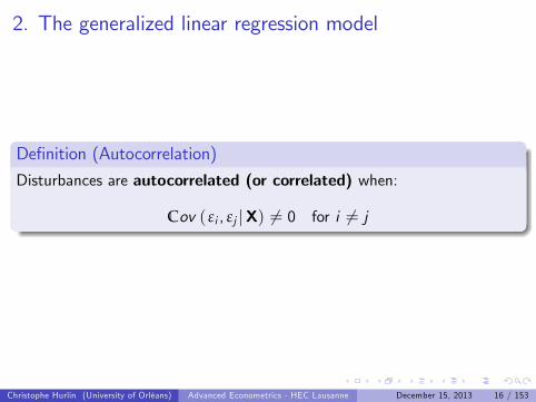
Denition (Autocorrelation)
Disturbances are autocorrelated (or correlated) when:
Cov ( εi , εj jX) 6= 0 for i 6= j
Christophe Hurlin (University of Orléans) Advanced Econometrics - HEC Lausanne December 15, 2013 16 / 153

2. The generalized linear regression model
Example (Autocorrelation)For instance, time-series data are usually homoscedastic, butautocorrelated, so Ω and Σ would be:
Σ =
0BB@σ2 σ12 .. σ1Nσ21 σ2 .. σ2N.. .. .. ..
σN1 .. .. σ2
1CCA = σ2Ω = σ2
0BB@1 ω12 .. ω1N
ω21 1 .. ω2N
.. .. .. ..ωN1 .. .. 1
1CCAwith ωij = σij/σ2 for i = 1, ..,N denotes the correlation (autocorrelation)
ωij =σijσ2= cor (εi , εj )
Christophe Hurlin (University of Orléans) Advanced Econometrics - HEC Lausanne December 15, 2013 17 / 153

2. The generalized linear regression model
Key Concepts
1 The generalized linear regression model
2 Heteroscedasticity
3 Autocorrelation (or correlation) of disturbances
Christophe Hurlin (University of Orléans) Advanced Econometrics - HEC Lausanne December 15, 2013 18 / 153

Section 3
Ine¢ ciency of the Ordinary Least Squares
Christophe Hurlin (University of Orléans) Advanced Econometrics - HEC Lausanne December 15, 2013 19 / 153

3. Ine¢ ciency of the Ordinary Least Squares
Objectives
The objective of this section are the following:
1 Study the properties of the OLS estimator in the generalized linearregression model
2 Study the nite sample properties of the OLS
3 Study the asymptotic properties of the OLS
4 Introduce the concept of robust / non-robust inference
Christophe Hurlin (University of Orléans) Advanced Econometrics - HEC Lausanne December 15, 2013 20 / 153

3. Ine¢ ciency of the Ordinary Least Squares
Introduction
Assume that the data are generated by the generalized linear regressionmodel:
y = Xβ+ ε
E (εjX) = 0N1V (εjX) = σ2Ω = Σ
Now consider the OLS estimator, denoted bβOLS , of the parameters β:
bβOLS = X>X1 X>yWe will study its nite sample and asymptotic properties.
Christophe Hurlin (University of Orléans) Advanced Econometrics - HEC Lausanne December 15, 2013 21 / 153

3. Ine¢ ciency of the Ordinary Least Squares
Denition (Assumption 3: Strict exogeneity of the regressors)The regressors are exogenous in the sense that:
E (εjX) = 0N1
Christophe Hurlin (University of Orléans) Advanced Econometrics - HEC Lausanne December 15, 2013 22 / 153

3. Ine¢ ciency of the Ordinary Least Squares
Finite sample properties of the OLS estimator
Christophe Hurlin (University of Orléans) Advanced Econometrics - HEC Lausanne December 15, 2013 23 / 153
3. Ine¢ ciency of the Ordinary Least Squares
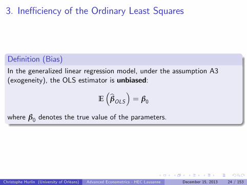
Denition (Bias)In the generalized linear regression model, under the assumption A3(exogeneity), the OLS estimator is unbiased:
EbβOLS = β0
where β0 denotes the true value of the parameters.
Christophe Hurlin (University of Orléans) Advanced Econometrics - HEC Lausanne December 15, 2013 24 / 153
3. Ine¢ ciency of the Ordinary Least Squares
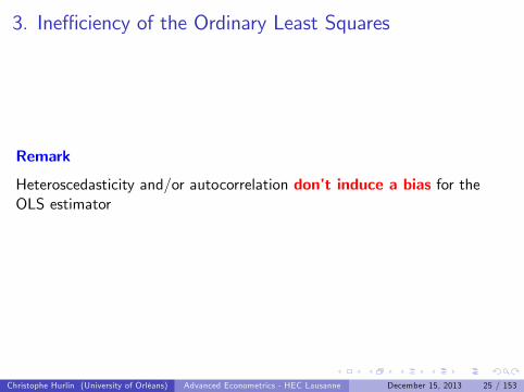
Remark
Heteroscedasticity and/or autocorrelation dont induce a bias for theOLS estimator
Christophe Hurlin (University of Orléans) Advanced Econometrics - HEC Lausanne December 15, 2013 25 / 153

3. Ine¢ ciency of the Ordinary Least Squares
Proof
bβOLS = X>X1 X>y = β0 +X>X
1 X>ε
So we have:
EbβOLS X = β0 +
X>X
1 X>E (εjX)
Under assumption A3 (exogeneity), E (εjX) = 0. Then, we get:
EbβOLS X = β0
Christophe Hurlin (University of Orléans) Advanced Econometrics - HEC Lausanne December 15, 2013 26 / 153

3. Ine¢ ciency of the Ordinary Least Squares
Proof (contd)
EbβOLS X = β0
So, we have:
EbβOLS = EX
EbβOLS X = EX (β0) = β0
where EX denotes the expectation with respect to the distribution of X.
The OLS estimator is unbiased:
EbβOLS = β0
Christophe Hurlin (University of Orléans) Advanced Econometrics - HEC Lausanne December 15, 2013 27 / 153

3. Ine¢ ciency of the Ordinary Least Squares
Denition (Bias)In the generalized linear regression model, under the assumption A3(exogeneity), the OLS estimator has a conditional variance covariancematrix given by
VbβOLS X = σ20
X>X
1X>ΩX
X>X
1and a variance covariance matrix given by:
VbβOLS = EX
VbβOLS X
Christophe Hurlin (University of Orléans) Advanced Econometrics - HEC Lausanne December 15, 2013 28 / 153

3. Ine¢ ciency of the Ordinary Least Squares
Proof
bβOLS = X>X1 X>y = β0 +X>X
1 X>ε
So we have:
VbβOLS X = E
X>X
1X>εε>X
X>X
1X=
X>X
1X>E
εε>
XX X>X1= σ20
X>X
1X>ΩX
X>X
1
Christophe Hurlin (University of Orléans) Advanced Econometrics - HEC Lausanne December 15, 2013 29 / 153
3. Ine¢ ciency of the Ordinary Least Squares
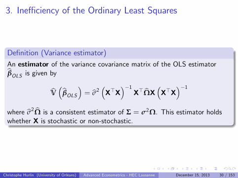
Denition (Variance estimator)An estimator of the variance covariance matrix of the OLS estimatorbβOLS is given by
bV bβOLS = bσ2 X>X1 X> bΩX X>X1where bσ2 bΩ is a consistent estimator of Σ = σ2Ω. This estimator holdswhether X is stochastic or non-stochastic.
Christophe Hurlin (University of Orléans) Advanced Econometrics - HEC Lausanne December 15, 2013 30 / 153

3. Ine¢ ciency of the Ordinary Least Squares
Denition (Normality assumption)
Under assumptions A3 (exogeneity) and A6 (normality), the OLSestimator obtained in the generalized linear regression model has an(exact) normal conditional distribution:
bβOLS X N β0, σ
2X>X
1X>ΩX
X>X
1
Christophe Hurlin (University of Orléans) Advanced Econometrics - HEC Lausanne December 15, 2013 31 / 153

3. Ine¢ ciency of the Ordinary Least Squares
Asymptotic properties of the OLS estimator
Christophe Hurlin (University of Orléans) Advanced Econometrics - HEC Lausanne December 15, 2013 32 / 153

3. Ine¢ ciency of the Ordinary Least Squares
Assumptions
plim1NX>X = Q
plim1NX>ΩX = Q
where:
1 Q is a K K nite (non null) denite positive matrix
2 Q is a K K nite (non null) denite positive matrix with
rank (Q) = K
Christophe Hurlin (University of Orléans) Advanced Econometrics - HEC Lausanne December 15, 2013 33 / 153
3. Ine¢ ciency of the Ordinary Least Squares
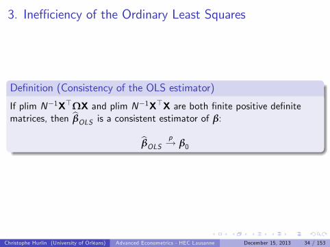
Denition (Consistency of the OLS estimator)
If plim N1X>ΩX and plim N1X>X are both nite positive denitematrices, then bβOLS is a consistent estimator of β:
bβOLS p! β0
Christophe Hurlin (University of Orléans) Advanced Econometrics - HEC Lausanne December 15, 2013 34 / 153

3. Ine¢ ciency of the Ordinary Least Squares
Proof
bβOLS = β0 +X>X
1 X>ε
We know that under assumption A3 (exogeneity):
plim1NX>ε = 0K1
plim1NX>X = Q
So, we haveplim bβOLS = β0
So, the estimator bβ is consistent. Christophe Hurlin (University of Orléans) Advanced Econometrics - HEC Lausanne December 15, 2013 35 / 153

3. Ine¢ ciency of the Ordinary Least Squares
Denition (Asymptotic distribution of the OLS)If the regressors are su¢ ciently well behaved and the o¤-diagonal terms indiminish su¢ ciently rapidly, then the least squares estimator isasymptotically normally distributed with
pNbβOLS β0
d! N
0, σ2Q1QQ1
where
Q = plim1NX>X Q = plim
1NX>ΩX
Christophe Hurlin (University of Orléans) Advanced Econometrics - HEC Lausanne December 15, 2013 36 / 153

3. Ine¢ ciency of the Ordinary Least Squares
Remark
1 Regularity conditions include the exogeneity conditions, but also (i)the regressors are su¢ ciently well-behaved and (ii) the o¤-diagonalterms of the variance-covariance matrix diminish su¢ ciently rapidly(relative to the diagonal elements).
2 For a formal proof in a general case, see Amemiya (1985, p. 187).
Amemiya T. (1985), Advanced Econometrics. Harvard University Press.
Christophe Hurlin (University of Orléans) Advanced Econometrics - HEC Lausanne December 15, 2013 37 / 153

3. Ine¢ ciency of the Ordinary Least Squares
Denition (Asymptotic variance)Under suitable regularity conditions, the asymptotic variance covariancematrix of the OLS estimator bβ is given by:
Vasy
bβOLS = σ2
NQ1QQ1
withQ = plim
1NX>X Q = plim
1NX>ΩX
Christophe Hurlin (University of Orléans) Advanced Econometrics - HEC Lausanne December 15, 2013 38 / 153

3. Ine¢ ciency of the Ordinary Least Squares
Fact (Non-robust inference)Because the variance of the least squares estimator is not
σ2X>X
1statistical inference (non-robust inference) based on
bσ2 X>X1 may be misleading. For instance the t-test-statistic:tβk =
bβkbσpmkkwhere mkk is kth diagonal element of X>X do not have a Studentdistribution.
Christophe Hurlin (University of Orléans) Advanced Econometrics - HEC Lausanne December 15, 2013 39 / 153

3. Ine¢ ciency of the Ordinary Least Squares
Robust / Non-robust inference
As a consequence, the familiar inference procedures based on the Fand t distributions will no longer be appropriate.
The question is to know how to estimate VbβOLS in the context
of the linear generalized regression model in order to make robustinference.
Christophe Hurlin (University of Orléans) Advanced Econometrics - HEC Lausanne December 15, 2013 40 / 153

3. Ine¢ ciency of the Ordinary Least Squares
Denition (Estimator of the asymptotic variance covariance matrix)
If Σ = σ2Ω were known, the consistent estimator of the (asymptotic)variance covariance of bβOLS would be:
bVasy
bβOLS = σ2
N
1NX>X
1 1NX>ΩX
1NX>X
1
Christophe Hurlin (University of Orléans) Advanced Econometrics - HEC Lausanne December 15, 2013 41 / 153

3. Ine¢ ciency of the Ordinary Least Squares
Proof
By denition:
Q = plim1NX>X
Q = plim1NX>ΩX
So,
plim bVasy
bβOLS = plimσ2
N
1NX>X
1 1NX>ΩX
1NX>X
1=
σ2
NQ1QQ1
Or equivalently bVasy
bβOLS p! Vasy
bβOLS
Christophe Hurlin (University of Orléans) Advanced Econometrics - HEC Lausanne December 15, 2013 42 / 153
3. Ine¢ ciency of the Ordinary Least Squares
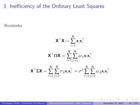
Reminder
X>X =N
∑i=1xix>i
X>ΩX =N
∑i=1
N
∑j=1
ωijxix>i
X>ΣX =N
∑i=1
N
∑j=1
σijxix>i = σ2N
∑i=1
N
∑j=1
ωijxix>i
Christophe Hurlin (University of Orléans) Advanced Econometrics - HEC Lausanne December 15, 2013 43 / 153

3. Ine¢ ciency of the Ordinary Least Squares
Remark
The estimator
bVasy
bβOLS = σ2
N
1NX>X
1 1NX>ΩX
1NX>X
1can also be written as
bVasy
bβOLS = σ2
N
1N
N
∑i=1xix>i
!1 1N
N
∑i=1
N
∑j=1
ωijxix>i
! 1N
N
∑i=1xix>i
!1
Christophe Hurlin (University of Orléans) Advanced Econometrics - HEC Lausanne December 15, 2013 44 / 153

3. Ine¢ ciency of the Ordinary Least Squares
Remark
In the next section, we will give a feasible estimator bVasy
bβOLS in thespecic case of an heteroscedastic model.
Christophe Hurlin (University of Orléans) Advanced Econometrics - HEC Lausanne December 15, 2013 45 / 153

3. Ine¢ ciency of the Ordinary Least Squares
Summary
In the GLR model, under some regularity conditions:
1 The OLS estimator is unbiased
2 The OLS estimator is (weakly) consistent
3 The OLS estimator is asymptotically normally distributed
Christophe Hurlin (University of Orléans) Advanced Econometrics - HEC Lausanne December 15, 2013 46 / 153

3. Ine¢ ciency of the Ordinary Least Squares
Summary
But...
1 The inference based on the estimator σ2X>X
1is misleading.
2 The OLS is ine¢ cient.
VbβOLS I1N (β0) is a positive denite matrix
Christophe Hurlin (University of Orléans) Advanced Econometrics - HEC Lausanne December 15, 2013 47 / 153

3. Ine¢ ciency of the Ordinary Least Squares
Key Concepts
1 OLS estimator in the generalized regression model
2 Finite sample properties
3 Asymptotic variance covariance matrix of the OLS estimator
Christophe Hurlin (University of Orléans) Advanced Econometrics - HEC Lausanne December 15, 2013 48 / 153

Section 4
Generalized Least Squares (GLS)
Christophe Hurlin (University of Orléans) Advanced Econometrics - HEC Lausanne December 15, 2013 49 / 153
4. Generalized Least Squares (GLS)
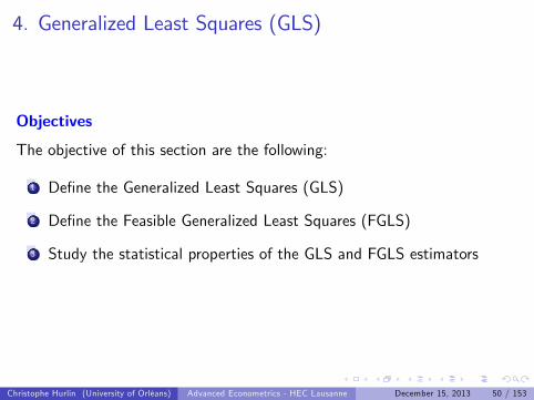
Objectives
The objective of this section are the following:
1 Dene the Generalized Least Squares (GLS)
2 Dene the Feasible Generalized Least Squares (FGLS)
3 Study the statistical properties of the GLS and FGLS estimators
Christophe Hurlin (University of Orléans) Advanced Econometrics - HEC Lausanne December 15, 2013 50 / 153
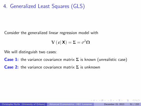
4. Generalized Least Squares (GLS)
Consider the generalized linear regression model with
V (εjX) = Σ = σ2Ω
We will distinguish two cases:
Case 1: the variance covariance matrix Σ is known (unrealistic case)
Case 2: the variance covariance matrix Σ is unknown
Christophe Hurlin (University of Orléans) Advanced Econometrics - HEC Lausanne December 15, 2013 51 / 153

4. Generalized Least Squares (GLS)
Case 1: Σ is known
The Generalized Least Squares (GLS) estimator
Christophe Hurlin (University of Orléans) Advanced Econometrics - HEC Lausanne December 15, 2013 52 / 153

4. Generalized Least Squares (GLS)
Denition (Factorisation)Since Ω is a positive denite matrix, it can factored as follows:
Ω = CΛC>
where the columns of C are the characteristics vectors of Ω, thecharacteristic roots of Ω are arrayed in the diagonal matrix Λ, and
C>C = CC> = IN
where I denotes the identity matrix.
Christophe Hurlin (University of Orléans) Advanced Econometrics - HEC Lausanne December 15, 2013 53 / 153

4. Generalized Least Squares (GLS)
DenitionWe dene the matrix P such that
P> = CΛ1/2
so thatΩ1 = P>P
Christophe Hurlin (University of Orléans) Advanced Econometrics - HEC Lausanne December 15, 2013 54 / 153

4. Generalized Least Squares (GLS)
ProofP> = CΛ1/2
Since Λ is diagonal, Λ1/2Λ1/2 = Λ1, and we have:
P>P = CΛ1/2Λ1/2C> = CΛ1C>
Consider the quantity P>PΩ:
P>PΩ = CΛ1C>CΛC>
= CΛ1ΛC>
= CC>
= IN
Since C satises CC> = IN . Then, P>P = Ω1
Christophe Hurlin (University of Orléans) Advanced Econometrics - HEC Lausanne December 15, 2013 55 / 153

4. Generalized Least Squares (GLS)GLS estimator
Premultiply the generalized linear regression model by P to obtain
Py = PXβ+Pε
or equivalentlyy = Xβ+ ε
The conditional variance of ε is
V (εjX) = E
εε>X
= PE
εε>XP>
= σ2PΩP>
= σ2Λ1/2C>CΛC>CΛ1/2
= σ2IN
Christophe Hurlin (University of Orléans) Advanced Econometrics - HEC Lausanne December 15, 2013 56 / 153

4. Generalized Least Squares (GLS)
GLS estimator (contd)
y = Xβ+ ε
V (εjX) = σ2IN
The classical regression model applies to this transformed model.
If Ω is assumed to be known, y = Py and X = PX are observed data.
So, we can apply the ordinary least squares to this transformed model:
bβ = X>X1 X>y
Christophe Hurlin (University of Orléans) Advanced Econometrics - HEC Lausanne December 15, 2013 57 / 153

4. Generalized Least Squares (GLS)
GLS estimator (contd)
bβ =X>X
1 X>y
=
X>P>PX
1 X>P>Py
=
X>Ω1X
1 X>Ω1y
This estimator is the generalized least squares (GLS) estimator of β.
Christophe Hurlin (University of Orléans) Advanced Econometrics - HEC Lausanne December 15, 2013 58 / 153

4. Generalized Least Squares (GLS)
Denition (GLS estimator)
The Generalized Least Squares (GLS) estimator of β is dened as to be:
bβGLS = X>Ω1X1
X>Ω1y
Christophe Hurlin (University of Orléans) Advanced Econometrics - HEC Lausanne December 15, 2013 59 / 153

4. Generalized Least Squares (GLS)
Denition (Bias)
Under the exogeneity assumption (A3), the estimator bβGLS is unbiased:EbβGLS = β0
where β0 denotes the true value of the parameters.
Christophe Hurlin (University of Orléans) Advanced Econometrics - HEC Lausanne December 15, 2013 60 / 153

4. Generalized Least Squares (GLS)
Proof
We have:
bβGLS = X>Ω1X1
X>Ω1y= β0 +
X>Ω1X
1 X>Ω1ε
So,
EbβGLS X = β0 +
X>Ω1X
1 X>Ω1E (εjX)
Under the exogeneity assumption A3, E (εjX) = 0, so we have
EbβGLS X = β0
andEbβGLS = EX
EbβGLS X = EX (β0) = β0
Christophe Hurlin (University of Orléans) Advanced Econometrics - HEC Lausanne December 15, 2013 61 / 153

4. Generalized Least Squares (GLS)
Denition (Variance covariance matrix)
The conditional variance covariance matrix of the estimator bβGLS isdened as to be:
VbβGLS X = σ2
X>Ω1X
1The variance covariance matrix is given by
VbβGLS = σ2EX
X>Ω1X
1
Christophe Hurlin (University of Orléans) Advanced Econometrics - HEC Lausanne December 15, 2013 62 / 153
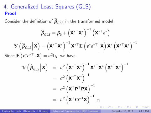
4. Generalized Least Squares (GLS)Proof
Consider the denition of bβGLS in the transformed model:bβGLS = β0 +
X>X
1 X>ε
VbβGLS X = X>X1 X>E
εε>
XX X>X1Since E
εε>
X = σ2IN , we have
VbβGLS X = σ2
X>X
1X>X
X>X
1= σ2
X>X
1= σ2
X>P>PX
1= σ2
X>Ω1X
1
Christophe Hurlin (University of Orléans) Advanced Econometrics - HEC Lausanne December 15, 2013 63 / 153
4. Generalized Least Squares (GLS)
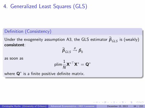
Denition (Consistency)
Under the exogeneity assumption A3, the GLS estimator bβGLS is (weakly)consistent: bβGLS p! β0
as soon asplim
1NX>X = Q
where Q is a nite positive denite matrix.
Christophe Hurlin (University of Orléans) Advanced Econometrics - HEC Lausanne December 15, 2013 64 / 153

4. Generalized Least Squares (GLS)
Proof
bβGLS = β0 +X>Ω1X
1 X>Ω1ε
Under the assumption A3 (exogeneity):
plim1NX>Ω1ε = 0K1
plim1NX>Ω1X = Q
So, we haveplim bβGLS = β0
The estimator bβGLS is weakly consistent. Christophe Hurlin (University of Orléans) Advanced Econometrics - HEC Lausanne December 15, 2013 65 / 153

4. Generalized Least Squares (GLS)
Denition (Asymptotic distribution)
Under some regularity conditions, the GLS estimator bβGLS isasymptotically normally distributed:
pNbβGLS β0
d! N
0, σ2Q1
where
Q = plim1NX>X = plim
1NX>Ω1X
Christophe Hurlin (University of Orléans) Advanced Econometrics - HEC Lausanne December 15, 2013 66 / 153
4. Generalized Least Squares (GLS)
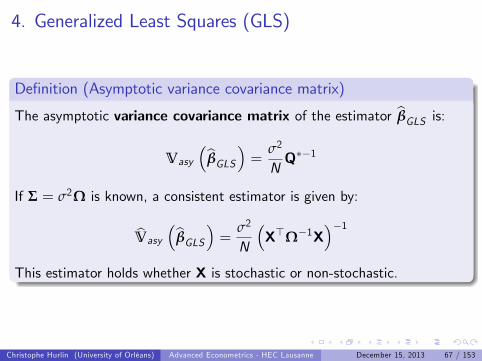
Denition (Asymptotic variance covariance matrix)
The asymptotic variance covariance matrix of the estimator bβGLS is:Vasy
bβGLS = σ2
NQ1
If Σ = σ2Ω is known, a consistent estimator is given by:
bVasy
bβGLS = σ2
N
X>Ω1X
1This estimator holds whether X is stochastic or non-stochastic.
Christophe Hurlin (University of Orléans) Advanced Econometrics - HEC Lausanne December 15, 2013 67 / 153
4. Generalized Least Squares (GLS)
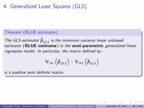
Theorem (BLUE estimator)
The GLS estimator bβGLS is the minimum variance linear unbiasedestimator (BLUE estimator) in the semi-parametric generalized linearregression model. In particular, the matrix dened by:
Vasy
bβOLSVasy
bβGLSis a positive semi denite matrix.
Christophe Hurlin (University of Orléans) Advanced Econometrics - HEC Lausanne December 15, 2013 68 / 153

4. Generalized Least Squares (GLS)
Theorem (E¢ ciency)Under suitable regularity conditions, in a parametric generalized linearregression model, the GLS estimator bβGLS is e¢ cient
VbβGLS = I1N (β0)
where I1N (β0) denotes the FDCR or Cramer-Rao bound.
Christophe Hurlin (University of Orléans) Advanced Econometrics - HEC Lausanne December 15, 2013 69 / 153
4. Generalized Least Squares (GLS)
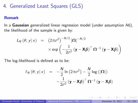
Remark
In a Gaussian generalized linear regression model (under assumption A6),the likelihood of the sample is given by:
LN (θ; y j x) =2πσ2
N/2 jΩjN/2
exp 12σ2
(yXβ)> Ω1 (yXβ)
The log-likelihood is dened as to be:
`N (θ; y j x) = N2ln2πσ2
N2log (jΩj)
12σ2
(yXβ)> Ω1 (yXβ)
Christophe Hurlin (University of Orléans) Advanced Econometrics - HEC Lausanne December 15, 2013 70 / 153

4. Generalized Least Squares (GLS)
Remark
For testing hypotheses, we can apply the full set of results in Chapter 4 tothe transformed model. For instance, for testing the p linear constraintsH0 : Rβ = q, the appropriate test-statistic is:
F =1p
Rbβ
GLS q
> σ2R
X>Ω1X
1R>1
RbβGLS q
Christophe Hurlin (University of Orléans) Advanced Econometrics - HEC Lausanne December 15, 2013 71 / 153

4. Generalized Least Squares (GLS)
FactTo summarize, all the results for the classical model, including the usualinference procedures, apply to the transformed model.
Christophe Hurlin (University of Orléans) Advanced Econometrics - HEC Lausanne December 15, 2013 72 / 153

4. Generalized Least Squares (GLS)
Case 2: Σ is unknown
The Feasible Generalized Least Squares (FGLS) estimator
Christophe Hurlin (University of Orléans) Advanced Econometrics - HEC Lausanne December 15, 2013 73 / 153

4. Generalized Least Squares (GLS)
Introduction
1 If Σ contains unknown parameters that must be estimated, thengeneralized least squares is not feasible.
2 With an unrestricted matrix Σ = σ2Ω, there are N (N + 1) /2additional parameters (since Σ is symmetric) to estimate
3 This number is far too many to estimate with N observations.
4 Obviously, some structure must be imposed on the model if we areto proceed.
Christophe Hurlin (University of Orléans) Advanced Econometrics - HEC Lausanne December 15, 2013 74 / 153

4. Generalized Least Squares (GLS)
Denition (Structure of variance covariance matrix)We assume that the conditional variance covariance matrix of thedisturbances can be expressed as a function of a small set of parameters α:
V (εjX) = σ2Ω (α)
Christophe Hurlin (University of Orléans) Advanced Econometrics - HEC Lausanne December 15, 2013 75 / 153

4. Generalized Least Squares (GLS)
Example (Time series)For instance, a commonly used formula in time-series settings is
Ω (ρ) =
0BBBBBB@
1 ρ ρ2 ρ3 .. ρN1
ρ 1 ρ ρ2 .. ρN2
ρ2 ρ 1 ρ .. ρN3
ρ3 ρ2 ρ 1 .. .... .. .. .. .. ..
ρN1 ρN2 ρN3 .. .. 1
1CCCCCCA
Christophe Hurlin (University of Orléans) Advanced Econometrics - HEC Lausanne December 15, 2013 76 / 153

4. Generalized Least Squares (GLS)
Example (Heteroscedascticity)If we consider a heteroscedastic model, where the variance of εi dependson a variable zi , with
V ( εi jX) = σ2zθi
we have
Ω (θ) =
0BBBB@zθ1 0 0 .. 00 zθ
2 0 .. 00 0 zθ
3 .. 0.. .. .. .. ..0 0 0 .. zθ
N
1CCCCA
Christophe Hurlin (University of Orléans) Advanced Econometrics - HEC Lausanne December 15, 2013 77 / 153

4. Generalized Least Squares (GLS)
Denition (Feasible Generalized Least Squares (FGLS))
Consider a consistent estimator bα of α, then the Feasible Least GeneralizedSquares (FGLS) estimator of β is dened as to be:
bβFGLS = X> bΩ1X1
X> bΩ1y
where bΩ = Ω (bα) is a consistent estimator of Ω (α) .
Christophe Hurlin (University of Orléans) Advanced Econometrics - HEC Lausanne December 15, 2013 78 / 153

4. Generalized Least Squares (GLS)
Remark
If
plim
1NX> bΩ1
X1NX>Ω1X
= 0
plim
1NX> bΩ1
y1NX>Ω1y
= 0
Then the GLS and FGLS estimators are asymptotically equivalent
bβFGLS bβGLS p! 0K1
Christophe Hurlin (University of Orléans) Advanced Econometrics - HEC Lausanne December 15, 2013 79 / 153

4. Generalized Least Squares (GLS)
Theorem (E¢ ciency)An asymptotically e¢ cient FGLS estimator does not require that we havean e¢ cient estimator of α; only a consistent one is required to achieve fulle¢ ciency for the FGLS estimator.
Christophe Hurlin (University of Orléans) Advanced Econometrics - HEC Lausanne December 15, 2013 80 / 153

4. Generalized Least Squares (GLS)
Remark
If the estimator bα is consistentbα p! α
then the FGLS estimator has the same asymptotic properties (consistency,e¢ ciency, asymptotic distribution etc.) than the GLS estimator.
Christophe Hurlin (University of Orléans) Advanced Econometrics - HEC Lausanne December 15, 2013 81 / 153

4. Generalized Least Squares (GLS)
Key Concepts
1 Factorisation of the variance covariance matrix
2 Generalized Least Squares (GLS) estimator
3 Feasible Generalized Least Squares (FGLS) estimator
Christophe Hurlin (University of Orléans) Advanced Econometrics - HEC Lausanne December 15, 2013 82 / 153

Section 5
Heteroscedasticity
Christophe Hurlin (University of Orléans) Advanced Econometrics - HEC Lausanne December 15, 2013 83 / 153

5. Heteroscedasticity
Objectives
The objective of this section are the following:
1 To determine the properties of the OLS in presence ofheteroscedasticity
2 To estimate the asymptotic variance covariance matrix of the OLSestimator in presence of heteroscedasticity
3 To introduce the concept of robust inference (to heteroscedasticity)
Christophe Hurlin (University of Orléans) Advanced Econometrics - HEC Lausanne December 15, 2013 84 / 153

5. Heteroscedasticity
Introduction
In the rest of this chapter, we will focus on the case of heteroscedasticdisturbances.
V ( εi jX) = σ2i for i = 1, ..,N
Heteroscedasticity arises in numerous applications, in both cross-sectionand time-series data.
For example, even after accounting for rm sizes, we expect to observegreater variation in the prots of large rms than in those of small ones.
Christophe Hurlin (University of Orléans) Advanced Econometrics - HEC Lausanne December 15, 2013 85 / 153

5. Heteroscedasticity
Assumption: We assume that the disturbances are pairwiseuncorrelated and heteroscedastic:
V (εjX) = Σ = σ2Ω
with
Σ =
0BB@σ21 0 .. 00 σ22 .. 0.. .. .. ..0 .. .. σ2N
1CCA = σ2Ω = σ2
0BB@ω1 0 .. 00 ω2 .. 0.. .. .. ..0 .. .. ωN
1CCAwith ωi = σ2i /σ2 for i = 1, ..,N.
Christophe Hurlin (University of Orléans) Advanced Econometrics - HEC Lausanne December 15, 2013 86 / 153
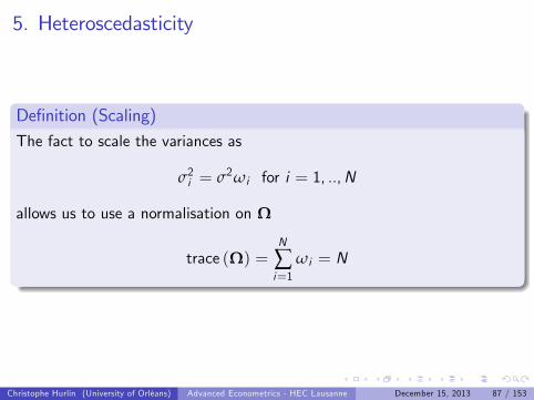
5. Heteroscedasticity
Denition (Scaling)The fact to scale the variances as
σ2i = σ2ωi for i = 1, ..,N
allows us to use a normalisation on Ω
trace (Ω) =N
∑i=1
ωi = N
Christophe Hurlin (University of Orléans) Advanced Econometrics - HEC Lausanne December 15, 2013 87 / 153

5. Heteroscedasticity
Introduction (contd)
We will consider three cases:
Case 1: the heteroscedasticity form (structure) is unknown: OLSestimator and robust inference
Case 2: the variance covariance matrix Σ is known: GLS or WeightedLeast Square (WLS)
Case 3: the variance covariance matrix Σ is unknown but its form(structure) is known: two-steps or iterated FGLS estimator
Christophe Hurlin (University of Orléans) Advanced Econometrics - HEC Lausanne December 15, 2013 88 / 153

5. Heteroscedasticity
Christophe Hurlin (University of Orléans) Advanced Econometrics - HEC Lausanne December 15, 2013 89 / 153

5. Heteroscedasticity
Case 1: Heteroscedasticity of unknown form
OLS and robust inference
Christophe Hurlin (University of Orléans) Advanced Econometrics - HEC Lausanne December 15, 2013 90 / 153

5. Heteroscedasticity
Assumption: We assume that the variances σ2i are unknown for i = 1, ..Nand no particular form (structure) is imposed on Ω (or Σ).
Christophe Hurlin (University of Orléans) Advanced Econometrics - HEC Lausanne December 15, 2013 91 / 153
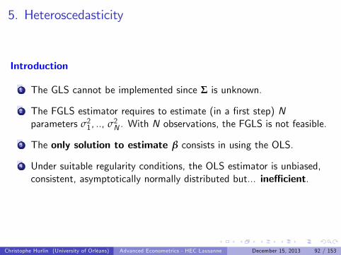
5. Heteroscedasticity
Introduction
1 The GLS cannot be implemented since Σ is unknown.
2 The FGLS estimator requires to estimate (in a rst step) Nparameters σ21, .., σ2N . With N observations, the FGLS is not feasible.
3 The only solution to estimate β consists in using the OLS.
4 Under suitable regularity conditions, the OLS estimator is unbiased,consistent, asymptotically normally distributed but... ine¢ cient.
Christophe Hurlin (University of Orléans) Advanced Econometrics - HEC Lausanne December 15, 2013 92 / 153
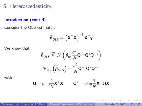
5. Heteroscedasticity
Introduction (contd)
Consider the OLS estimator:
bβOLS = X>X1 X>yWe know that bβOLS asy N
β0,
σ2
NQ1QQ1
Vasy
bβOLS = σ2
NQ1QQ1
withQ = plim
1NX>X Q = plim
1NX>ΩX
Christophe Hurlin (University of Orléans) Advanced Econometrics - HEC Lausanne December 15, 2013 93 / 153

5. Heteroscedasticity
Problem (Robust inference with OLS)The conventionally estimated covariance matrix for the least squares
estimator σ2X>X
1is inappropriate; the appropriate matrix is
σ2X>X
1 X>ΩX
1 X>X
1. It is unlikely that these two would
coincide, so the usual estimators of the standard errors are likely to be
erroneous. The inference (test-statistics) based σ2X>X
1is
misleading.
Christophe Hurlin (University of Orléans) Advanced Econometrics - HEC Lausanne December 15, 2013 94 / 153

5. Heteroscedasticity
Question
How to estimate Vasy
bβOLS and to make robust inference?Vasy
bβOLS = σ2
NQ1QQ1
Q = plim1NX>X Q = plim
1NX>ΩX
Christophe Hurlin (University of Orléans) Advanced Econometrics - HEC Lausanne December 15, 2013 95 / 153

5. Heteroscedasticity
We seek an estimator for
Q = plim1NX>ΩX = plim
1N
N
∑i=1
ωixix>i = EX
ωixix>i
or equivalently of
Q = plim1NX>ΣX = plim
1N
N
∑i=1
σ2i xix>i = EX
σixix>i
with
Q = σ2Q
Christophe Hurlin (University of Orléans) Advanced Econometrics - HEC Lausanne December 15, 2013 96 / 153
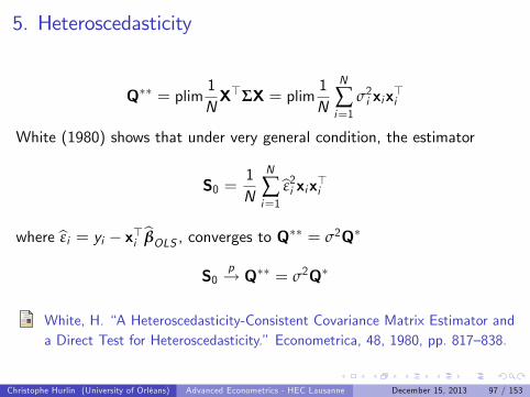
5. Heteroscedasticity
Q = plim1NX>ΣX = plim
1N
N
∑i=1
σ2i xix>i
White (1980) shows that under very general condition, the estimator
S0 =1N
N
∑i=1
bε2i xix>iwhere bεi = yi x>i bβOLS , converges to Q = σ2Q
S0p! Q = σ2Q
White, H. A Heteroscedasticity-Consistent Covariance Matrix Estimator anda Direct Test for Heteroscedasticity.Econometrica, 48, 1980, pp. 817838.
Christophe Hurlin (University of Orléans) Advanced Econometrics - HEC Lausanne December 15, 2013 97 / 153

5. Heteroscedasticity
Vasy
bβOLS = σ2
NQ1QQ1
We know that:
S0 =1N
N
∑i=1
bε2i xix>i p! σ2Q
1NX>X
1=
1N
N
∑i=1xix>i
!1p! Q1
So,1N
1NX>X
1S0
1NX>X
1p! Vasy
bβOLS
Christophe Hurlin (University of Orléans) Advanced Econometrics - HEC Lausanne December 15, 2013 98 / 153

5. Heteroscedasticity
Denition (White heteroscedasticity consistent estimator)The White consistent estimator of the asymptotic variance-covariancematrix of the ordinary least squares estimator bβOLS in the generalizedlinear regression model is dened to be:
bVasy
bβOLS = N X>X1 S0 X>X1bVasy
bβOLS p! Vasy
bβOLSwith
S0 =1N
N
∑i=1
bε2i xix>i
Christophe Hurlin (University of Orléans) Advanced Econometrics - HEC Lausanne December 15, 2013 99 / 153

5. Heteroscedasticity
Corollary (White heteroscedasticity consistent estimator)The White consistent estimator can written as:
bVasy
bβOLS = 1N
1N
N
∑i=1xix>i
!1 1N
N
∑i=1
bε2i xix>i!
1N
N
∑i=1xix>i
!1
Christophe Hurlin (University of Orléans) Advanced Econometrics - HEC Lausanne December 15, 2013 100 / 153

5. Heteroscedasticity
Remarks
1 This result is extremely important and useful. It implies that withoutactually specifying the type of heteroscedasticity, we can still makeappropriate inferences based on the results of least squares.
2 This implication is especially useful if we are unsure of the precisenature of the heteroscedasticity (which is probably most of the time).
Christophe Hurlin (University of Orléans) Advanced Econometrics - HEC Lausanne December 15, 2013 101 / 153

5. Heteroscedasticity
Christophe Hurlin (University of Orléans) Advanced Econometrics - HEC Lausanne December 15, 2013 102 / 153

5. Heteroscedasticity
Remark
Given the normalisation trace(Ω) = N, we have:
σ2 =1N
N
∑i=1
σ2i
Christophe Hurlin (University of Orléans) Advanced Econometrics - HEC Lausanne December 15, 2013 103 / 153

5. Heteroscedasticity
Denition (SSR)
The least squares estimator bσ2 dened by:bσ2 = bε>bε
N K =1
N KN
∑i=1
bε2iconverges to the probability limit of the average variance of thedisturbances bσ2 p! lim
N!∞σ2 = lim
N!∞
1N
N
∑i=1
σ2i
Christophe Hurlin (University of Orléans) Advanced Econometrics - HEC Lausanne December 15, 2013 104 / 153

5. Heteroscedasticity
Example (White robust estimator. Source: Greene (2012))Consider the generalized linear regression model:
AVGEXPi = β1 + β2AGEi + β3Ownrenti + β4Incomei + β5Income2i + εi
where AVGEXP denotes the Avg. monthly credit card expenditure,Ownrent denotes a binary variable (individual owns (1) or rents (0) home),Age denotes the age in years, Income denotes the income divided by10,000. The data are available in le Chapter5_data.xls. Question:write a Matlab code to (1) estimate the parameters by OLS, (2) computethe standard errors and the robust standard errors and (3) compare yourresults with Eviews.
Christophe Hurlin (University of Orléans) Advanced Econometrics - HEC Lausanne December 15, 2013 105 / 153

5. Heteroscedasticity
Christophe Hurlin (University of Orléans) Advanced Econometrics - HEC Lausanne December 15, 2013 106 / 153

5. Heteroscedasticity
1 2 3 4 5 6 7 8 9 10500
0
500
1000
1500
2000
Income
OLS
resi
dual
s
This graph is the sign of heteroscedasticity.. the variance of the residualsseems to depend on the income.
Christophe Hurlin (University of Orléans) Advanced Econometrics - HEC Lausanne December 15, 2013 107 / 153

5. Heteroscedasticity
The values are the same.. perfect
Christophe Hurlin (University of Orléans) Advanced Econometrics - HEC Lausanne December 15, 2013 108 / 153

5. Heteroscedasticity
The values are di¤erent... Why?
Christophe Hurlin (University of Orléans) Advanced Econometrics - HEC Lausanne December 15, 2013 109 / 153

5. Heteroscedasticity
Remark
This di¤erence is due to the fact that Eviews uses a nite samplecorrection for S0 (Davidson and MacKinnon, 1993)
S0 =1
N KN
∑i=1
bε2i xix>iDavidson, R. and J. MacKinnon. Estimation and Inference in Econometrics.New York: Oxford University Press, 1993.
Christophe Hurlin (University of Orléans) Advanced Econometrics - HEC Lausanne December 15, 2013 110 / 153

5. Heteroscedasticity
Christophe Hurlin (University of Orléans) Advanced Econometrics - HEC Lausanne December 15, 2013 111 / 153

5. Heteroscedasticity
The values are now identical.
Christophe Hurlin (University of Orléans) Advanced Econometrics - HEC Lausanne December 15, 2013 112 / 153

5. Heteroscedasticity
Case 2: Heteroscedasticity with known Σ
GLS and Weighted Least Squares
Christophe Hurlin (University of Orléans) Advanced Econometrics - HEC Lausanne December 15, 2013 113 / 153
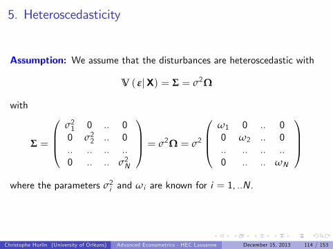
5. Heteroscedasticity
Assumption: We assume that the disturbances are heteroscedastic with
V (εjX) = Σ = σ2Ω
with
Σ =
0BB@σ21 0 .. 00 σ22 .. 0.. .. .. ..0 .. .. σ2N
1CCA = σ2Ω = σ2
0BB@ω1 0 .. 00 ω2 .. 0.. .. .. ..0 .. .. ωN
1CCAwhere the parameters σ2i and ωi are known for i = 1, ..N.
Christophe Hurlin (University of Orléans) Advanced Econometrics - HEC Lausanne December 15, 2013 114 / 153

5. Heteroscedasticity
Denition (GLS estimator)
In presence of heteroscedasticity, the Generalized Least Squares (GLS)estimator of β is dened as to:
bβGLS =
N
∑i=1
xix>iωi
!1 N
∑i=1
xiyiωi
!
or equivalently by
bβGLS =
N
∑i=1
xix>iσ2i
!1 N
∑i=1
xiyiσ2i
!
Christophe Hurlin (University of Orléans) Advanced Econometrics - HEC Lausanne December 15, 2013 115 / 153

5. HeteroscedasticityProof
In general, whatever the form of Σ = σ2Ω, we have:
bβGLS = X>Ω1X1
X>Ω1y
Since Ω is diagonal:
X>Ω1X =N
∑i=1
xix>iωi
X>Ω1y =N
∑i=1
xiyiωi
As a consequence:
bβGLS =
N
∑i=1
xix>iωi
!1 N
∑i=1
xiyiωi
!
Christophe Hurlin (University of Orléans) Advanced Econometrics - HEC Lausanne December 15, 2013 116 / 153

5. Heteroscedasticity
Remark
bβGLS =
N
∑i=1
xix>iωi
!1 N
∑i=1
xiyiωi
!This formula is similar to that obtained for a Weighted Least Squares(WLS).
bβWLS =
N
∑i=1
δixix>i
!1 N
∑i=1
δixiyi
!
Christophe Hurlin (University of Orléans) Advanced Econometrics - HEC Lausanne December 15, 2013 117 / 153

5. Heteroscedasticity
Fact (GLS and WLS)In presence of heteroscedasticity, the GLS estimator is a particular case ofthe Weighted Least Squares (WLS) estimator.
bβWLS =
N
∑i=1
δixix>i
!1 N
∑i=1
δixiyi
!
where δi is an arbitrary weight. For δi = 1/ωi , we have bβWLS = bβGLS .
Christophe Hurlin (University of Orléans) Advanced Econometrics - HEC Lausanne December 15, 2013 118 / 153

5. Heteroscedasticity
Remark
1 The WLS estimator is consistent regardless of the weights used, aslong as the weights are uncorrelated with the disturbances.
2 In general, we consider a weight which is proportional to oneexplicative variable (the income in the last example):
σ2i = σ2x2ik () δi =1x2ik
Christophe Hurlin (University of Orléans) Advanced Econometrics - HEC Lausanne December 15, 2013 119 / 153

5. Heteroscedasticity
Case 3: Heteroscedasticity for a given structure
FGLS and two-step or iterated estimators
Christophe Hurlin (University of Orléans) Advanced Econometrics - HEC Lausanne December 15, 2013 120 / 153

5. Heteroscedasticity
Assumption: We assume that the disturbances are heteroscedastic with
V (εjX) = Σ (α) = σ2Ω (α)
where α denotes a set of parameters.
Christophe Hurlin (University of Orléans) Advanced Econometrics - HEC Lausanne December 15, 2013 121 / 153

5. Heteroscedasticity
Example (Restriction)We assume that
V ( εi jX) = σ2i (α) = σ2z>i α
2where α = (α1 : .. : αH )
> is a H 1 vector of parameters and zi is H 1of explicative variables (not necessarily the same as in xi ).
Christophe Hurlin (University of Orléans) Advanced Econometrics - HEC Lausanne December 15, 2013 122 / 153

5. Heteroscedasticity
Example (Harveys (1976) restriction)
Harvey (1976) considers a restriction of the form:
V ( εi jX) = σ2i (α) = expx>i α
where α = (α1 : .. : αH )
> is a H 1 vector of parameters and zi is H 1of explicative variables (not necessarily the same as in xi ).
Christophe Hurlin (University of Orléans) Advanced Econometrics - HEC Lausanne December 15, 2013 123 / 153

5. Heteroscedasticity
We know that the GLS estimator is dened by:
bβGLS =
N
∑i=1
xix>iσ2i (α)
!1 N
∑i=1
xiyiσ2i (α)
!
S, the feasible GLS (FGLS) estimator is:
bβFGLS =
N
∑i=1
xix>iσ2i (bα)
!1 N
∑i=1
xiyiσ2i (bα)
!
Christophe Hurlin (University of Orléans) Advanced Econometrics - HEC Lausanne December 15, 2013 124 / 153

5. Heteroscedasticity
If we assume for instance that
V ( εi jX) = σ2i (α) = expz>i α
where zi is a vector of H variables, a way to estimate α consists inconsidering the model:
lnbε2i = z>i α+ vi
and to estimate α by OLS. The OLS is consistent even it is ine¢ cient (dueto the heteroscedasticity). Given bα, we have a consistent estimator for σ2i :
bσ2i = expz>i bα p! σ2i (α)
Christophe Hurlin (University of Orléans) Advanced Econometrics - HEC Lausanne December 15, 2013 125 / 153

5. Heteroscedasticity
ProblemIn order to estimate β by the GLS, we need bα, and to estimate α, we needthe residuals bεi = yi x>i bβGLS ...
Christophe Hurlin (University of Orléans) Advanced Econometrics - HEC Lausanne December 15, 2013 126 / 153

5. Heteroscedasticity
Two solutions
1 A two steps FGLS estimator
2 An iterative FGLS estimator
Christophe Hurlin (University of Orléans) Advanced Econometrics - HEC Lausanne December 15, 2013 127 / 153

5. Heteroscedasticity
Denition (Two-steps FGLS estimator)
First step: estimate the parameters β by OLS. Compute the residualsbεi = yi x>i bβOLS and estimate the parameters α according to theappropriate model. Second step: compute the estimated variances σ2i (bα)and compute the FGLS estimator:
bβFGLS =
N
∑i=1
xix>iσ2i (bα)
!1 N
∑i=1
xiyiσ2i (bα)
!
Christophe Hurlin (University of Orléans) Advanced Econometrics - HEC Lausanne December 15, 2013 128 / 153
5. Heteroscedasticity
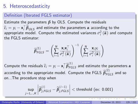
Denition (Iterated FGLS estimator)
Estimate the parameters β by OLS. Compute the residualsbεi = yi x>i bβOLS and estimate the parameters α according to theappropriate model. Compute the estimated variances σ2i (bα) and computethe FGLS estimator:
bβ(1)FGLS =
N
∑i=1
xix>iσ2i (bα)
!1 N
∑i=1
xiyiσ2i (bα)
!
Compute the residuals bεi = yi x>i bβ(1)FGLS and estimate the parameters α
according to the appropriate model. Compute the FGLS bβ(2)FGLS and soon...The procedure stop when
supj=1,..,K
bβ(i )j ,FGLS bβ(i1)j ,FGLS
< threshold (ex: 0.001)Christophe Hurlin (University of Orléans) Advanced Econometrics - HEC Lausanne December 15, 2013 129 / 153

5. Heteroscedasticity
Example (Harveys (1976) multiplicative model of heteroscedasticity)Consider the generalized linear regression model:
AVGEXPi = β1 + β2AGEi + β3Ownrenti + β4Incomei + β5Income2i + εi
where the heteroscedasticity satises the Harveys (1976) specication
V ( εi jX) = σ2i = exp (α1 + α2Incomei )
The data are available in le Chapter5_data.xls. Question: write aMatlab code to estimate the parameters by FGLS by using a two-step andan iterative estimator.
Christophe Hurlin (University of Orléans) Advanced Econometrics - HEC Lausanne December 15, 2013 130 / 153

5. Heteroscedasticity
Remark
A way to get the estimates of the parameters α1 and α2 is to consider theregression:
lnbε2i = α1 + α2Incomei + vi
and to estimate the parameters by OLS.
Christophe Hurlin (University of Orléans) Advanced Econometrics - HEC Lausanne December 15, 2013 131 / 153
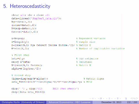
5. Heteroscedasticity
Christophe Hurlin (University of Orléans) Advanced Econometrics - HEC Lausanne December 15, 2013 132 / 153

5. Heteroscedasticity
Christophe Hurlin (University of Orléans) Advanced Econometrics - HEC Lausanne December 15, 2013 133 / 153

5. Heteroscedasticity
Christophe Hurlin (University of Orléans) Advanced Econometrics - HEC Lausanne December 15, 2013 134 / 153

5. Heteroscedasticity
Christophe Hurlin (University of Orléans) Advanced Econometrics - HEC Lausanne December 15, 2013 135 / 153

5. Heteroscedasticity
Key Concepts
1 OLS and robust inference
2 White heteroscedasticity consistent estimator
3 GLS and Weighted Least Squares (WLS)
4 FGLS: two-steps and iterated estimators
Christophe Hurlin (University of Orléans) Advanced Econometrics - HEC Lausanne December 15, 2013 136 / 153

Section 6
Testing for Heteroscedasticity
Christophe Hurlin (University of Orléans) Advanced Econometrics - HEC Lausanne December 15, 2013 137 / 153

6. Testing for heteroscedasticity
Objectives
The objective of this section are to introduce the following tests forheteroscedasticity:
1 White general test
2 The Breusch-Pagan / Godfrey LM test
Christophe Hurlin (University of Orléans) Advanced Econometrics - HEC Lausanne December 15, 2013 138 / 153

6. Testing for heteroscedasticity
Denition (White test for heteroscedasticity)The White test for heteroscedasticity is based on:
H0 : σ2i = σ2 for i = 1, ..,N
H1 : σ2i 6= σ2j for at least one pair (i , j)
Christophe Hurlin (University of Orléans) Advanced Econometrics - HEC Lausanne December 15, 2013 139 / 153

6. Testing for heteroscedasticity
The intuition of the test is based on the following idea:
1 If there is no heteroscedasticity (under the null H0):
Vasy
bβOLS = σ2Q1
bVasy
bβOLS = σ2X>X
12 Under the alternative (heteroscedasticity):
Vasy
bβOLS = σ2Q1QQ1
bVasy
bβOLS = σ2X>X
1X>ΩX
X>X
1
Christophe Hurlin (University of Orléans) Advanced Econometrics - HEC Lausanne December 15, 2013 140 / 153

6. Testing for heteroscedasticity
White (1980) proposes the following procedure and test-statistic:
Step 1: Estimation of the model using the OLS estimator of β.
Step 2: Determine the residuals bεi = yi x>i bβOLS .Step 3: Regress bε2i on a constant and all unique columns vectors containedin X and all the squares and cross-products of the column vectors in X.
Step 4: Determine the coe¢ cient of determination, R2, of the previousregression.
Christophe Hurlin (University of Orléans) Advanced Econometrics - HEC Lausanne December 15, 2013 141 / 153

6. Testing for heteroscedasticity
Denition (White test for heteroscedasticity)
Under the null, the White test-statistic NR2 converges:
N R2 d!H0
χ2 (m 1)
where m is the number of explanatory variables in the regression of bε2i .The critical region of size α is
W =y : N R2 > χ21α
where χ21α denotes the 1-α critical value of the χ2 (m 1) distribution.
Christophe Hurlin (University of Orléans) Advanced Econometrics - HEC Lausanne December 15, 2013 142 / 153

6. Testing for heteroscedasticity
Example (Whites (1980) test for heteroscedasticity)Consider the generalized linear regression model:
AVGEXPi = β1 + β2AGEi + β3Ownrenti + β4Incomei + β5Income2i + εi
The data are available in le Chapter5_data.xls. Question: write aMatlab code to compute the White test-statistic for heteroscedasticity andits p-value. What is you conclusion for a signicance level of 5%?Compare your results with Eviews.
Christophe Hurlin (University of Orléans) Advanced Econometrics - HEC Lausanne December 15, 2013 143 / 153

6. Testing for heteroscedasticity
Christophe Hurlin (University of Orléans) Advanced Econometrics - HEC Lausanne December 15, 2013 144 / 153

6. Testing for heteroscedasticity
Christophe Hurlin (University of Orléans) Advanced Econometrics - HEC Lausanne December 15, 2013 145 / 153

6. Testing for heteroscedasticity
Denition (Breusch and Pagan test)
Breusch and Pagan (1979) have devised a Lagrange multiplier test ofthe hypothesis that
σ2i = σ2f
α0 + z>i α
where zi = (zi1..zip)> is a p 1 vector of independent variables. The test
is:H0 : α = 0p1 (homoscedasticity)
H1 : α 6= 0p1 (heteroscedasticity)
Christophe Hurlin (University of Orléans) Advanced Econometrics - HEC Lausanne December 15, 2013 146 / 153

6. Testing for heteroscedasticity
The test can be carried out with a simple regression of
gi = Nbε2ibε>bε 1 = N bε2i
∑Ni=1bε2i 1
on the variables zik for k = 1, .,N and a constant term.
gi = α0 + α1zi1 + ...+ αpzip + vi
Christophe Hurlin (University of Orléans) Advanced Econometrics - HEC Lausanne December 15, 2013 147 / 153

6. Testing for heteroscedasticity
Denition (Breusch and Pagan test-statistic)
Dene Z the N (p + 1) matrix of observations on (1, zi ) and let g bethe N 1 vector of observations
gi = Nbε2ibε>bε 1
Then, the Breusch and Pagans test-statistic is dened by:
LM =12g>Z
Z>Z
1Z>g
Under the null, we have:LM
d!H0
χ2 (p)
Christophe Hurlin (University of Orléans) Advanced Econometrics - HEC Lausanne December 15, 2013 148 / 153

6. Testing for heteroscedasticity
Example (Breusch and Pagans (1979) test for heteroscedasticity)Consider the generalized linear regression model:
AVGEXPi = β1 + β2AGEi + β3Ownrenti + β4Incomei + β5Income2i + εi
The data are available in le Chapter5_data.xls. Question: write aMatlab code to compute the Breusch and Pagan test-statistic forheteroscedasticity with zi = xi and its p-value. What is you conclusion fora signicance level of 5%?
Christophe Hurlin (University of Orléans) Advanced Econometrics - HEC Lausanne December 15, 2013 149 / 153

6. Testing for heteroscedasticity
Christophe Hurlin (University of Orléans) Advanced Econometrics - HEC Lausanne December 15, 2013 150 / 153

6. Testing for heteroscedasticity
Christophe Hurlin (University of Orléans) Advanced Econometrics - HEC Lausanne December 15, 2013 151 / 153

6. Testing for heteroscedasticity
Key Concepts
1 White test for heteroscedasticity
2 Breusch and Pagan test for heteroscedasticity
Christophe Hurlin (University of Orléans) Advanced Econometrics - HEC Lausanne December 15, 2013 152 / 153

End of Chapter 5
Christophe Hurlin (University of Orléans)
Christophe Hurlin (University of Orléans) Advanced Econometrics - HEC Lausanne December 15, 2013 153 / 153