This chapter is part of Precalculus. by OpenStax College, © 2014 Rice University.

This material is licensed under a Creative Commons CC-BY-SA license.

Chapter 5: Systems of Equations

Section 5.1: Systems in Two Variables ...................................................................... 303 Section 5.1 Exercises .................................................................................................. 319 Section 5.2: Systems in Three Variables .................................................................... 322 Section 5.2 Exercises ................................................................................................. 333 Section 5.3: Linear Inequalities .................................................................................. 336

Section 5.3: Exercises ………………………………………………………………. 342

Section 5.4: Solving Systems using Matrices ............................................................. 343 Section 5.4 Exercises .................................................................................................. 356 Section 5.5: Matrices and Matrix Operations ............................................................. 359 Section 5.5 Exercises ................................................................................................. 371

Section 5.1: Systems in Two Variables

Back when studying linear equations, we found the intersection of two lines. Doing so

allowed us to solve interesting problems by finding a pair of values that satisfied two

different equations. While we didn't call it this at the time, we were solving a system of

equations. To start out, we'll review an example of the type of problem we've solved

before.

Example 1

A small business produces soap and lotion gift baskets. Labor, utilities, and other fixed

expenses cost $6,000 a month. Each basket costs $8 to produce, and sells for $20. How

many baskets does the company need to sell each month to break even?

In business terms, "break even" means for revenue (money brought in) to equal costs.

While this problem can be approached in several ways, we'll approach here by first

creating two linear functions, one for the costs, and another for revenue.

Let's define n to be the number of gift baskets the company sells in a month. There are

$6,000 of fixed costs each month, and costs increase by $8 for each basket, so we can

write the linear function for costs, C, as

( ) 6000 8C n n

Each sale brings in $20, so the revenue, R, after selling n baskets will be:

( ) 20R n n

Chapter 5 304

To find the break-even point, we are looking for

the number of baskets where the revenue will

equal the costs. In other words, if we were to

graph the two linear functions, we are looking

for the point that lies on both lines; the solution

is the point that satisfies both equations.

In this case we could probably solve the

problem from the graph itself, but we can also

solve it algebraically by setting the equations

equal:

( ) ( )R n C n

20 6000 8n n Subtract 8n from

both sides

12 6000n Divide

6000500

12n Evaluate either function at this input

(500) (500) 10,000R C

The break-even point is at 500 baskets. The company must sell 500 baskets a month, at

which point their revenue of $10,000 will cover their total costs of $10,000.

The example above illustrates one type of system of equations, one where both equations

are given in functional form. When the equations are written this way, it is easy to solve

the system using substitution, by setting the two outputs equal, and solving for the input.

However, many system of equations problems aren't written this way.

Example 2

A company produces a basic and premium version of its product. The basic version

requires 20 minutes of assembly and 15 minutes of painting. The premium version

requires 30 minutes of assembly and 30 minutes of painting. If the company has

staffing for 3,900 minutes of assembly and 3,300 minutes of painting each week. If the

company wants to fully utilize all staffed hours, how many of each item should they

produce?

Notice first that this problem has two variables, or two unknowns - the number of basic

products to make, and the number of premium products to make. There are also two

constraints - the hours of assembly and the hours of painting available. This is going to

give us two equations in two unknowns, what we call a 2 by 2 system of equations.

We'll start by defining our variables:

b: the number of basic products produced

p: the number of premium products produced

Section 5.1 Systems in Two Variables 305

Now we can create our equations based on the constraints. Each basic product requires

20 minutes of assembly, so producing b items will require 20b minutes. Each premium

product requires 30 minutes of assembly, so producing p items will require 30p

minutes. Together we have 3,900 minutes available, giving us the equation:

20 30 3900b p

Using the same approach for painting gives the equation

15 30 3300b p

Together, these form our system of equations. They are sometimes written as a pair

with a curly bracket on the left to indicate that they should be considered as connected

equations.

20 30 3900

15 30 3300

b p

b p

As before, our goal is to find a pair of values, (b, p), that satisfies both equations. We'll

return to this problem and solve it shortly.

While it may not be clear, the equation 20 30 3900b p we constructed above is a

linear equation, like the linear equations from the first example, it's just written

differently. We could, if desired, solve this equation for p to get it written in slope-

intercept form:

30 3900 20p b , so 2

1303

p b

We typically don't do this, since it often makes the system harder to solve then when

using other techniques. To dive into this further, let's first clarify what it means to find a

solution to a system of linear equations.

System of Linear Equations

A system of linear equations consists of two or more linear equations made up of two or

more variables such that all equations in the system are considered simultaneously.

A solution to a system is a set of numerical values for each variable in the system that

will satisfy all equations in the system at the same time.

Not every system will have exactly one solution, but we'll look more closely at that later.

To check to see if an ordered pair is a solution to a system of equations, you would:

1. Substitute the ordered pair into each equation in the system.

2. Determine whether true statements result from the substitution in both equations;

if so, the ordered pair is a solution.

Chapter 5 306

Example 3 (video example here)

Determine whether the ordered pair 5,1 is a solution to the given system of equations.

3 8

2 9

x y

x y

Substitute the ordered pair 5,1 into both equations.

(5) 3(1) 8

8 8 True

2(5) 9 (1)

1=1 True

The ordered pair 5,1 satisfies both equations, so it is the solution to the system.

There are three common methods for solving systems of linear equations with two

variables. The first is solving by graphing. In the first example above we graphed both

equations, and the solution to the system was the intersection of the lines.

Example 4

Solve the following system of equations by graphing.

2 8

1

x y

x y

Solve the first equation for .y

2 8

2 8

x y

y x

Solve the second equation for .y

1

1

x y

y x

Graph both equations on the same set of axes. The

lines appear to intersect at the point 3, 2 . We can

check to make sure that this is the solution to the

system by substituting the ordered pair into both

equations. 2( 3) ( 2) 8

8 8 True

( 3) ( 2) 1

1 1 True

The solution to the system is the ordered pair 3, 2 .

Section 5.1 Systems in Two Variables 307

Try it Now 1

Solve the following system of equations by graphing.

2 5 25

4 5 35

x y

x y

While this method can work well enough when the solution values are both integers, it is

not very useful when the intersection is not at a clear point. Additionally, it requires

solving both equations for y, which adds extra steps. Because of these limitations,

solving by graphing is rarely used, but can be useful for checking whether your algebraic

answers are reasonable.

Solving a System by Substitution Another method for solving a system of equations is the substitution method, in which we

solve one of the equations for one variable and then substitute the result into the second

equation to solve for the second variable.

Solving a system using substitution

1. Solve one of the two equations for one of the variables in terms of the other.

2. Substitute the expression for this variable into the second equation, then solve for

the remaining variable.

3. Substitute that solution into either of the original equations to find the value of the

first variable. If possible, write the solution as an ordered pair.

4. Check the solution in both equations.

The problem we did in Example 1 was technically done by substitution, but it was made

easier since both equations were already solved for one variable, y. An example of a

more typical case is shown next.

Example 5 (video example here)

Solve the following system of equations by substitution.

5

2 5 1

x y

x y

First, we will solve the first equation for .y

5

5

x y

y x

Now we can substitute the expression 5x for y in the second equation.

Chapter 5 308

Now, we substitute 8x into the first equation and solve for .y

8 5

3

y

y

Our solution is 8,3 .

We can check the solution by substituting 8,3 into both equations.

Try it Now 2

2. Solve the following system of equations by substitution.

3

4 3 2

x y

x y

Substitution can always be used, but is an especially good choice when one of the

variables in one of the equations has a coefficient of 1 or -1, making it easy to solve for

that variable without introducing fractions. This is fairly common in many applications.

Video Example 1: Application of Systems of Equations

Example 6

Julia has just retired, and has $600,000 in her retirement account that she needs to

reallocate to produce income. She is looking at two investments: a very safe

guaranteed annuity that will provide 3% interest, and a somewhat riskier bond fund that

averages 7% interest. She would like to invest as little as possible in the riskier bond

fund, but needs to produce $40,000 a year in interest to live on. How much should she

invest in each account?

Notice there are two unknowns in this problem: the amount she should invest in the

annuity and the amount she should invest in the bond fund. We can start by defining

variables for the unknowns:

2 5 1

2 5 5 1

2 5 25 1

3 24

8

x y

x x

x x

x

x

5

(8) (3) 5 True

2 5 1

2 8 5 3 1 True

x y

x y

Section 5.1 Systems in Two Variables 309

a: The amount (in dollars) she invests in the annuity

b: The amount (in dollars) she invests in the bond fund.

Our first equation comes from noting that together she is going to invest $600,000:

600,000a b

Our second equation will come from the interest. She earns 3% on the annuity, so the

interest earned in a year would be 0.03a. Likewise, the interest earned on the bond fund

in a year would be 0.07b. Together, these need to total $40,000, giving the equation:

0.03 0.07 40,000a b

Together, these two equations form our system. The first equation is an ideal candidate

for the first step of substitution - we can easily solve the equation for a or b:

600,000a b

Then we can substitute this expression for a in the second equation and solve.

0.03(600,000 ) 0.07 30,000b b

18,000 0.03 0.07 40,000b b

0.04 22,000b

550,000b

Now substitute this back into the equation 600,000a b to find a

600,000 550,000

50,000

a

a

In order to reach her goal, Julia will have to invest $550,000 in the bond fund, and

$50,000 in the annuity.

Solving a System by the Addition Method

A third method of solving systems of linear equations is the addition method, also called

the elimination method. In this method, we add two terms with the same variable, but

opposite coefficients, so that the sum is zero. Of course, not all systems are set up with

the two terms of one variable having opposite coefficients. Often we must adjust one or

both of the equations by multiplication so that one variable will be eliminated by

addition.

Chapter 5 310

Solving a System by the Addition Method

1. Write both equations with x- and y-variables on the left side of the equal sign and

constants on the right.

2. Write one equation above the other, lining up corresponding variables. If one of

the variables in the top equation has the opposite coefficient of the same variable

in the bottom equation, add the equations together, eliminating one variable. If

not, use multiplication by a nonzero number so that one of the variables in the top

equation has the opposite coefficient of the same variable in the bottom equation,

then add the equations to eliminate the variable.

3. Solve the resulting equation for the remaining variable.

4. Substitute that value into one of the original equations and solve for the second

variable.

5. Check the solution by substituting the values into the other equation.

Example 7

Solve the given system of equations by addition.

2 1

3

x y

x y

Both equations are already set equal to a constant. Notice that the coefficient of x in

the second equation, –1, is the opposite of the coefficient of x in the first equation, 1.

We can add the two equations to eliminate x without needing to multiply by a constant.

2 1

3

3 2

x y

x y

y

Now that we have eliminated ,x we can solve the resulting equation for .y

3 2

23

y

y

Then, we substitute this value for y into one of the original equations and solve for .x

3

2 33

233

73

73

x y

x

x

x

x

Section 5.1 Systems in Two Variables 311

The solution to this system is 7 2, .3 3

Check the solution in the first equation.

2 1

7 223 3

7 43 3

33

1 1 True

x y

Often using the addition method will require multiplying one or both equations by a

constant so terms will eliminate.

Example 8

Solve the given system of equations by the addition method.

3 5 11

2 11

x y

x y

Adding these equations as presented will not eliminate a variable. However, we see that

the first equation has 3x in it and the second equation has .x So if we multiply the

second equation by 3, the x -terms will add to zero.

2 11

3 2 3 11 Multiply both sides by 3.

3 6 33 Use the distributive property.

x y

x y

x y

Now, let’s add them.

3 5 11

3 6 33

11 44

4

x y

x y

y

y

For the last step, we substitute 4y into one of the original equations and solve for

.x

3 5 11

3 5 4 11

3 20 11

3 9

3

x y

x

x

x

x

Chapter 5 312

Our solution is the ordered pair 3, 4 .

Check the solution in the original second equation.

2 11

3 2 4 3 8

11 True

x y

Try it Now 3

3. Solve the system of equations by addition.

2 7 2

3 20

x y

x y

Example 9

Solve the given system of equations in two variables by addition.

2 3 16

5 10 30

x y

x y

One equation has 2x and the other has 5 .x The least common multiple is 10x so we

will have to multiply both equations by a constant in order to eliminate one variable.

Let’s eliminate x by multiplying the first equation by 5 and the second equation by

2.

5 2 3 5 16

10 15 80

2 5 10 2 30

10 20 60

x y

x y

x y

x y

Then, we add the two equations together.

10 15 80

10 20 60

35 140

4

x y

x y

y

y

Substitute 4y into the original first equation.

2 3 4 16

2 12 16

2 4

2

x

x

x

x

Section 5.1 Systems in Two Variables 313

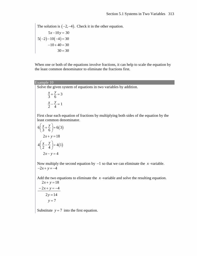
The solution is 2, 4 . Check it in the other equation.

5 10 30

5 2 10 4 30

10 40 30

30 30

x y

When one or both of the equations involve fractions, it can help to scale the equation by

the least common denominator to eliminate the fractions first.

Example 10

Solve the given system of equations in two variables by addition.

33 6

12 4

yx

yx

First clear each equation of fractions by multiplying both sides of the equation by the

least common denominator.

6 6 33 6

2 18

4 4 12 4

2 4

yx

x y

yx

x y

Now multiply the second equation by 1 so that we can eliminate the x -variable.

2 4x y

Add the two equations to eliminate the x -variable and solve the resulting equation. 2 18

2 4

2 14

7

x y

x y

y

y

Substitute 7y into the first equation.

Chapter 5 314

2 7 18

2 11

11 7.52

x

x

x

The solution is 11,7 .2

Check it in the other equation.

12 4

1172 1

2 4

11 7 14 4

4 14

yx

Try it Now

4. Solve the system of equations by addition.

2 3 8

3 5 10

x y

x y

Using these approaches, we can revisit the equation from Example 2

Example 11

In Example 2, we set up the system below. Solve it.

20 30 3900

15 30 3300

b p

b p

Adding the equations would not eliminate a variable, but we notice that the coefficients

on p are the same, so multiplying one of the equations by -1 will change the sign of the

coefficients. Multiplying the second equation by -1 gives the system

20 30 3900

15 30 3300

b p

b p

Adding these equations gives

5 600

120

b

b

Substituting b = 30 into the first equation,

Section 5.1 Systems in Two Variables 315

20(120) 30 3900

2400 30 3900

30 1500

50

p

p

p

p

The solution is b = 120, p = 50, meaning the company should produce 120 basic

products and 50 premium products to full utilize staffed hours.

Checking our answer in the second equation:

15(120) 30(50) 3300

1800 1500 3300

3300 3300

Dependent and Inconsistent Systems

Up until now, we have only considered cases where there is exactly one solution to the

system. We can categorize systems of linear equations by the number of solutions. A

consistent system of equations has at least one solution. A consistent system is

considered to be an independent system if it has a single solution, such as the examples

we just explored. The two lines have different slopes and intersect at one point in the

plane. A consistent system is considered to be a dependent system if the equations have

the same slope and the same y-intercepts. In other words, the lines coincide so the

equations represent the same line. Every point on the line represents a coordinate pair that

satisfies the system. Thus, there are an infinite number of solutions.

Another type of system of linear equations is an inconsistent system, which is one in

which the equations represent two parallel lines. The lines have the same slope and

different y-intercepts. There are no points common to both lines; hence, there is no

solution to the system.

Types of Linear Systems

An independent system has exactly one solution pair , .x y The point where the

two lines intersect is the only solution.

An inconsistent system has no solution. Notice that the two lines are parallel and

will never intersect.

A dependent system has infinitely many solutions. The lines are coincident. They

are the same line, so every coordinate pair on the line is a solution to both

equations.

Chapter 5 316

Independent System

Inconsistent System

Dependent System

We can use substitution or addition to identify inconsistent systems. Recall that an

inconsistent system consists of parallel lines that have the same slope but different y-

intercepts. They will never intersect. When searching for a solution to an inconsistent

system, we will come up with a false statement, such as 12 0.

Example 12 (video example here)

Solve the following system of equations.

9 2

2 13

x y

x y

We can approach this problem in two ways. Because one equation is already solved for

,x the most obvious step is to use substitution.

2 13

9 2 2 13

9 0 13

9 13

x y

y y

y

Clearly, this statement is a contradiction (a false statement) because 9 13. Therefore,

the system has no solution, and the system is inconsistent.

The second approach would be to first manipulate the equations so that they are both in

slope-intercept form. We manipulate the first equation as follows.

9 2

2 9

1 92 2

x y

y x

y x

We then convert the second equation expressed to slope-intercept form.

2 13

2 13

1 132 2

x y

y x

y x

Section 5.1 Systems in Two Variables 317

Comparing the equations, we see that they have the same slope but different y-

intercepts. Therefore, the lines are parallel and do not intersect.

1 92 2

1 132 2

y x

y x

Recall that a dependent system of equations in two variables is a system in which the two

equations represent the same line. Dependent systems have an infinite number of

solutions because all of the points on one line are also on the other line. After using

substitution or addition, the resulting equation will be an identity, such as 0 0.

Example 13

Find a solution to the system of equations using the addition method.

3 2

3 9 6

x y

x y

With the addition method, we want to eliminate one of the variables by adding the

equations. In this case, let’s focus on eliminating .x If we multiply both sides of the first

equation by 3, then we will be able to eliminate the x-variable.

3 2

( 3) 3 3 2 Multiply both sides of the equation by 3.

3 9 6

x y

x y

x y

3 9 6

3 9 6

0 0

x y

x y

We can see that there will be an infinite number of solutions that satisfy both equations.

In some cases, realizing there are an infinite number of solutions is enough, and we can

stop there. In other cases, we will want to describe the set of solutions. One way is to

simply say it's the set of points that satisfy 3 2x y , but often we would solve that

equation for y and describe the solution as set of points 1 2

, .3 3

x x

Like with the inconsistent system, if we rewrote both equations in the slope-intercept

form we might know what the solution would look like before adding. Let’s look at

what happens when we convert the system to slope-intercept form.

Chapter 5 318

3 2

3 2

1 23 3

3 9 6

9 3 6

3 69 9

1 23 3

x y

y x

y x

x y

y x

y x

y x

Notice the results are the same. The general solution to the system is 1 2

, .3 3

x x

Try it Now

5. Solve the systems:

a. 2 2 2

2 2 6

y x

y x

b.

2 5

3 6 15

y x

y x

Try it Now Answers

1. The solution to the system is the ordered pair 5,3 .

2. 2, 5

3. 6, 2

4. 10,-4( )

5a. No solution. The system is inconsistent.

5b. The system is dependent so there are infinite solutions of the form ( ,2 5).x x

Section 5.1 Systems in Two Variables 319

Section 5.1 Exercises

For the following exercises, determine whether the given ordered pair is a solution to the

system of equations.

1. 5 4

6 2

x y

x y

and )0,4( 2.

104

1353

yx

yx and )1,6(

3. 042

173

yx

yx and )3,2( 4.

792

752

yx

yx and )1,1(

5. 123

438

yx

yx and )5,3(

For the following exercises, solve each system by substitution.

6. 432

53

yx

yx7.

10105

1823

yx

yx

8. 093

1024

yx

yx9.

3.159

8.342

yx

yx

10. 8.163

2.132

yx

yx11.

5210

12.0

yx

yx

12. 905030

953

yx

yx13.

8412

23

yx

yx

14.

94

1

6

1

163

1

2

1

yx

yx

15.

33

1

8

1

112

3

4

1

yx

yx

For the following exercises, solve each system by addition.

16. 3027

4252

yx

yx17.

462

3456

yx

yx

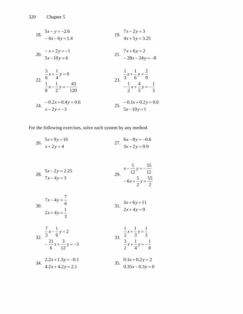
Chapter 5 320

18. 4.164

6.25

yx

yx 19.

25.354

327

yx

yx

20. 6105

12

yx

yx 21.

82428

267

yx

yx

22.

120

43

2

1

8

1

04

1

6

5

yx

yx

23.

3

1

5

4

2

1

9

2

6

1

3

1

yx

yx

24. 32

6.04.02.0

yx

yx 25.

1105

6.02.01.0

yx

yx

For the following exercises, solve each system by any method.

26. 42

1695

yx

yx 27.

9.023

6.086

yx

yx

28. 347

25.225

yx

yx 29.

2

55

2

56

12

55

12

5

yx

yx

30.

3

142

6

747

yx

yx

31. 942

1163

yx

yx

32.

312

3

6

21

26

1

3

7

yx

yx

33.

8

1

4

1

2

3

3

1

3

1

2

1

yx

yx

34. 1.22.42.4

1.03.12.2

yx

yx 35.

03.035.0

22.01.0

yx

yx

Section 5.1 Systems in Two Variables 321

For the following exercises, graph the system of equations and state whether the system

is consistent, inconsistent, or dependent and whether the system has one solution, no

solution, or infinite solutions.

36. 3.12

6.03

yx

yx37.

142

42

yx

yx

38. 1262

72

yx

yx39.

32

753

yx

yx

40. 1569

523

yx

yx

For the following exercises, solve for the desired quantity.

41. A stuffed animal business has a total cost of production and a

revenue function Find the break-even point.

42. A fast-food restaurant has a cost of production and a revenue

function When does the company start to turn a profit?

43. A cell phone factory has a cost of production and a revenue

function What is the break-even point?

44. A musician charges where is the total number of

attendees at the concert. The venue charges $80 per ticket. After how many

people buy tickets does the venue break even, and what is the value of the total

tickets sold at that point?

45. A guitar factory has a cost of production The price of each

guitar is $325. Write the revenue function. Determine the number of guitars the

company needs to sell to break even? What is the cost and the revenue when they

break even?

46. For the following exercises, use a system of linear equations with two variables

and two equations to solve.

47. A moving company charges a flat rate of $150, and an additional $5 for each box.

If a taxi service would charge $20 for each box, how many boxes would you need

for it to be cheaper to use the moving company, and what would be the total cost?

48. If a scientist mixed 10% saline solution with 60% saline solution to get 25 gallons

of 40% saline solution, how many gallons of 10% and 60% solutions were mixed?

C =12x+ 3020 .R x

C(x) =11x+120

( ) 5 .R x x

( ) 150 10,000C x x

( ) 200 .R x x

( ) 64 20,000,C x x x

( ) 75 50,000.C x x