chapter 5 student lecture notes 5-1 · probability distributions normal uniform exponential....
TRANSCRIPT

Business Statistics: A Decision-Making Approach, 6e © 2005 Prentice-Hall, Inc.
Chapter 5 Student Lecture Notes 5-1
Business Statistics: A Decision-Making Approach, 6e © 2005 Prentice-Hall, Inc. Chap 5-1
Business Statistics: A Decision-Making Approach
6th Edition
Chapter 5Discrete and Continuous Probability Distributions
Business Statistics: A Decision-Making Approach, 6e © 2005 Prentice-Hall, Inc. Chap 5-2
Chapter Goals
After completing this chapter, you should be able to:Apply the binomial distribution to applied problemsCompute probabilities for the Poisson and hypergeometric distributions
Find probabilities using a normal distribution table and apply the normal distribution to business problems
Recognize when to apply the uniform and exponential distributions
Business Statistics: A Decision-Making Approach, 6e © 2005 Prentice-Hall, Inc. Chap 5-3
Probability Distributions
ContinuousProbability
Distributions
Binomial
Hypergeometric
Poisson
Probability Distributions
DiscreteProbability
Distributions
Normal
Uniform
Exponential

Business Statistics: A Decision-Making Approach, 6e © 2005 Prentice-Hall, Inc.
Chapter 5 Student Lecture Notes 5-2
Business Statistics: A Decision-Making Approach, 6e © 2005 Prentice-Hall, Inc. Chap 5-4
A discrete random variable is a variable that can assume only a countable number of valuesMany possible outcomes:
number of complaints per daynumber of TV’s in a householdnumber of rings before the phone is answered
Only two possible outcomes:gender: male or femaledefective: yes or nospreads peanut butter first vs. spreads jelly first
Discrete Probability Distributions
Business Statistics: A Decision-Making Approach, 6e © 2005 Prentice-Hall, Inc. Chap 5-5
Continuous Probability Distributions
A continuous random variable is a variable that can assume any value on a continuum (can assume an uncountable number of values)
thickness of an itemtime required to complete a tasktemperature of a solutionheight, in inches
These can potentially take on any value, depending only on the ability to measure accurately.
Business Statistics: A Decision-Making Approach, 6e © 2005 Prentice-Hall, Inc. Chap 5-6
The Binomial Distribution
Binomial
Hypergeometric
Poisson
Probability Distributions
DiscreteProbability
Distributions
Business Statistics: A Decision-Making Approach, 6e © 2005 Prentice-Hall, Inc.
Chapter 5 Student Lecture Notes 5-3
Business Statistics: A Decision-Making Approach, 6e © 2005 Prentice-Hall, Inc. Chap 5-7
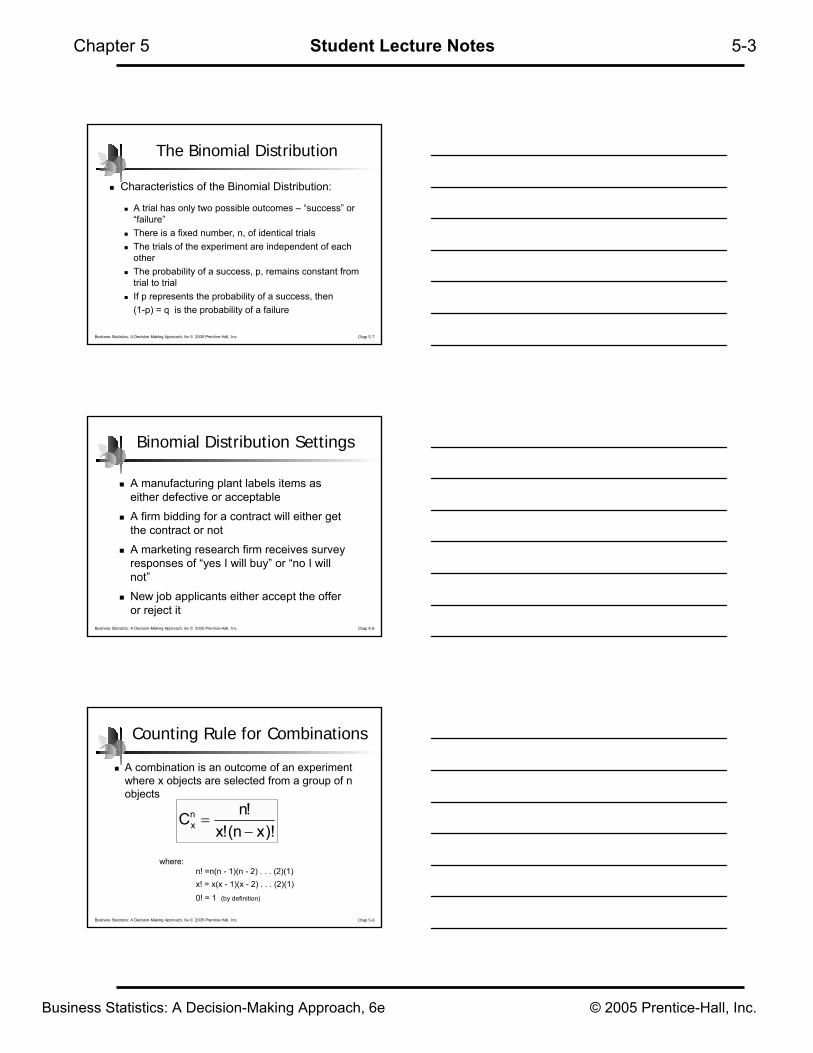
The Binomial Distribution
Characteristics of the Binomial Distribution:
A trial has only two possible outcomes – “success” or “failure”There is a fixed number, n, of identical trialsThe trials of the experiment are independent of each otherThe probability of a success, p, remains constant from trial to trialIf p represents the probability of a success, then (1-p) = q is the probability of a failure
Business Statistics: A Decision-Making Approach, 6e © 2005 Prentice-Hall, Inc. Chap 5-8
Binomial Distribution Settings
A manufacturing plant labels items as either defective or acceptable
A firm bidding for a contract will either get the contract or not
A marketing research firm receives survey responses of “yes I will buy” or “no I will not”
New job applicants either accept the offer or reject it
Business Statistics: A Decision-Making Approach, 6e © 2005 Prentice-Hall, Inc. Chap 5-9
Counting Rule for Combinations
A combination is an outcome of an experiment where x objects are selected from a group of n objects
)!xn(!x!nCn
x −=
where:n! =n(n - 1)(n - 2) . . . (2)(1)x! = x(x - 1)(x - 2) . . . (2)(1)
0! = 1 (by definition)
Business Statistics: A Decision-Making Approach, 6e © 2005 Prentice-Hall, Inc.
Chapter 5 Student Lecture Notes 5-4
Business Statistics: A Decision-Making Approach, 6e © 2005 Prentice-Hall, Inc. Chap 5-10
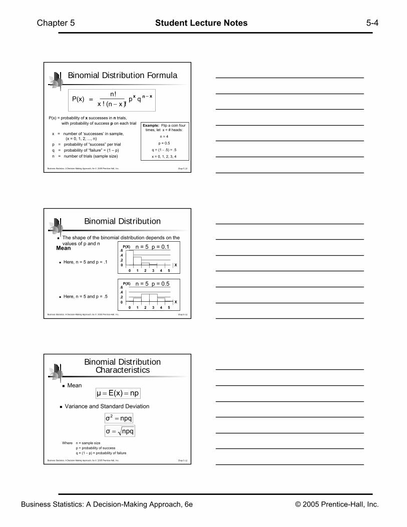
P(x) = probability of x successes in n trials,with probability of success p on each trial
x = number of ‘successes’ in sample, (x = 0, 1, 2, ..., n)
p = probability of “success” per trialq = probability of “failure” = (1 – p)n = number of trials (sample size)
P(x)n
x ! n xp qx n x!
( )!=
−−
Example: Flip a coin four times, let x = # heads:
n = 4
p = 0.5
q = (1 - .5) = .5
x = 0, 1, 2, 3, 4
Binomial Distribution Formula
Business Statistics: A Decision-Making Approach, 6e © 2005 Prentice-Hall, Inc. Chap 5-11
n = 5 p = 0.1
n = 5 p = 0.5
Mean
0.2.4.6
0 1 2 3 4 5X
P(X)
.2
.4
.6
0 1 2 3 4 5X
P(X)
0
Binomial Distribution
The shape of the binomial distribution depends on the values of p and n
Here, n = 5 and p = .1
Here, n = 5 and p = .5
Business Statistics: A Decision-Making Approach, 6e © 2005 Prentice-Hall, Inc. Chap 5-12
Binomial Distribution Characteristics
Mean
Variance and Standard Deviation
npE(x)µ ==
npqσ2 =
npqσ =
Where n = sample sizep = probability of successq = (1 – p) = probability of failure
Business Statistics: A Decision-Making Approach, 6e © 2005 Prentice-Hall, Inc.
Chapter 5 Student Lecture Notes 5-5
Business Statistics: A Decision-Making Approach, 6e © 2005 Prentice-Hall, Inc. Chap 5-13
n = 5 p = 0.1
n = 5 p = 0.5
Mean
0.2.4.6
0 1 2 3 4 5X
P(X)
.2
.4
.6
0 1 2 3 4 5X
P(X)
0
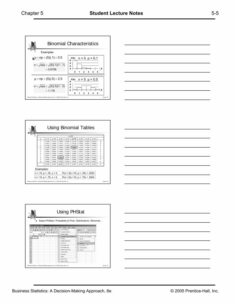
0.5(5)(.1)npµ ===
0.6708
.1)(5)(.1)(1npqσ
=
−==
2.5(5)(.5)npµ ===
1.118.5)(5)(.5)(1npqσ
=
−==
Binomial Characteristics
Examples
Business Statistics: A Decision-Making Approach, 6e © 2005 Prentice-Hall, Inc. Chap 5-14
Using Binomial Tables
xp=.50p=.55p=.60p=.65p=.70p=.75p=.80p=.85
109876543210
0.00100.00980.04390.11720.20510.24610.20510.11720.04390.00980.0010
0.00250.02070.07630.16650.23840.23400.15960.07460.02290.00420.0003
0.00600.04030.12090.21500.25080.20070.11150.04250.01060.00160.0001
0.01350.07250.17570.25220.23770.15360.06890.02120.00430.00050.0000
0.02820.12110.23350.26680.20010.10290.03680.00900.00140.00010.0000
0.05630.18770.28160.25030.14600.05840.01620.00310.00040.00000.0000
0.10740.26840.30200.20130.08810.02640.00550.00080.00010.00000.0000
0.19690.34740.27590.12980.04010.00850.00120.00010.00000.00000.0000
012345678910
p=.50p=.45p=.40p=.35p=.30p=.25p=.20p=.15x
n = 10
Examples: n = 10, p = .35, x = 3: P(x = 3|n =10, p = .35) = .2522
n = 10, p = .75, x = 2: P(x = 2|n =10, p = .75) = .0004
Business Statistics: A Decision-Making Approach, 6e © 2005 Prentice-Hall, Inc. Chap 5-15
Using PHStat
Select PHStat / Probability & Prob. Distributions / Binomial…
Business Statistics: A Decision-Making Approach, 6e © 2005 Prentice-Hall, Inc.
Chapter 5 Student Lecture Notes 5-6
Business Statistics: A Decision-Making Approach, 6e © 2005 Prentice-Hall, Inc. Chap 5-16
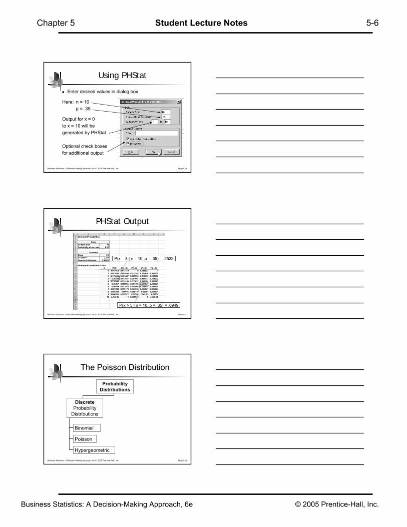
Using PHStat
Enter desired values in dialog box
Here: n = 10p = .35
Output for x = 0 to x = 10 will be generated by PHStat
Optional check boxesfor additional output
Business Statistics: A Decision-Making Approach, 6e © 2005 Prentice-Hall, Inc. Chap 5-17
P(x = 3 | n = 10, p = .35) = .2522
PHStat Output
P(x > 5 | n = 10, p = .35) = .0949
Business Statistics: A Decision-Making Approach, 6e © 2005 Prentice-Hall, Inc. Chap 5-18
The Poisson Distribution
Binomial
Hypergeometric
Poisson
Probability Distributions
DiscreteProbability
Distributions
Business Statistics: A Decision-Making Approach, 6e © 2005 Prentice-Hall, Inc.
Chapter 5 Student Lecture Notes 5-7
Business Statistics: A Decision-Making Approach, 6e © 2005 Prentice-Hall, Inc. Chap 5-19
The Poisson Distribution
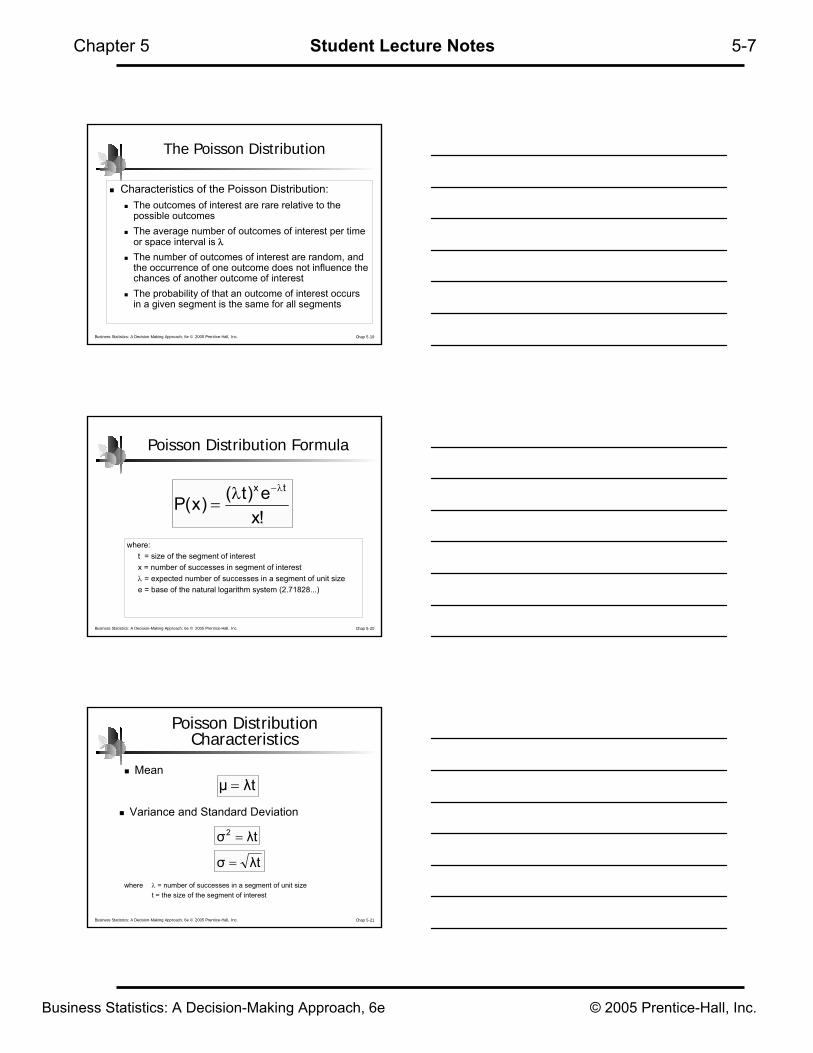
Characteristics of the Poisson Distribution:The outcomes of interest are rare relative to the possible outcomesThe average number of outcomes of interest per time or space interval is λThe number of outcomes of interest are random, and the occurrence of one outcome does not influence the chances of another outcome of interestThe probability of that an outcome of interest occurs in a given segment is the same for all segments
Business Statistics: A Decision-Making Approach, 6e © 2005 Prentice-Hall, Inc. Chap 5-20
Poisson Distribution Formula
where:t = size of the segment of interest x = number of successes in segment of interestλ = expected number of successes in a segment of unit sizee = base of the natural logarithm system (2.71828...)
!xe)t()x(P
tx λ−λ=
Business Statistics: A Decision-Making Approach, 6e © 2005 Prentice-Hall, Inc. Chap 5-21
Poisson Distribution Characteristics
Mean
Variance and Standard Deviation
λtµ =
λtσ2 =
λtσ =where λ = number of successes in a segment of unit size
t = the size of the segment of interest
Business Statistics: A Decision-Making Approach, 6e © 2005 Prentice-Hall, Inc.
Chapter 5 Student Lecture Notes 5-8
Business Statistics: A Decision-Making Approach, 6e © 2005 Prentice-Hall, Inc. Chap 5-22
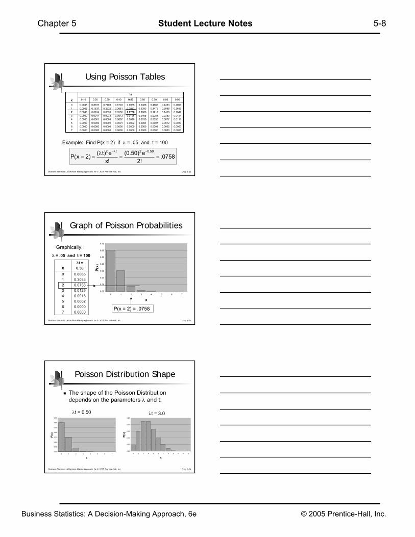
Using Poisson Tables
λt
0.90
0.40660.36590.16470.04940.01110.00200.00030.0000
0.44930.35950.14380.03830.00770.00120.00020.0000
0.49660.34760.12170.02840.00500.00070.00010.0000
0.54880.32930.09880.01980.00300.00040.00000.0000
0.60650.30330.07580.01260.00160.00020.00000.0000
0.67030.26810.05360.00720.00070.00010.00000.0000
0.74080.22220.03330.00330.00030.00000.00000.0000
0.81870.16370.01640.00110.00010.00000.00000.0000
0.90480.09050.00450.00020.00000.00000.00000.0000
01234567
0.800.700.600.500.400.300.200.10X
Example: Find P(x = 2) if λ = .05 and t = 100
.07582!
e(0.50)!xe)t()2x(P
0.502tx
==λ
==−λ−
Business Statistics: A Decision-Making Approach, 6e © 2005 Prentice-Hall, Inc. Chap 5-23
Graph of Poisson Probabilities
0.00
0.10
0.20
0.30
0.40
0.50
0.60
0.70
0 1 2 3 4 5 6 7
x
P(x)
01234567
X0.60650.30330.07580.01260.00160.00020.00000.0000
λt =0.50
P(x = 2) = .0758
Graphically:λ = .05 and t = 100
Business Statistics: A Decision-Making Approach, 6e © 2005 Prentice-Hall, Inc. Chap 5-24
Poisson Distribution Shape
The shape of the Poisson Distribution depends on the parameters λ and t:
0.00
0.05
0.10
0.15
0.20
0.25
1 2 3 4 5 6 7 8 9 10 11 12
x
P(x)
0.00
0.10
0.20
0.30
0.40
0.50
0.60
0.70
0 1 2 3 4 5 6 7
x
P(x)
λt = 0.50 λt = 3.0
Business Statistics: A Decision-Making Approach, 6e © 2005 Prentice-Hall, Inc.
Chapter 5 Student Lecture Notes 5-9
Business Statistics: A Decision-Making Approach, 6e © 2005 Prentice-Hall, Inc. Chap 5-25
The Hypergeometric Distribution
Binomial
Poisson
Probability Distributions
DiscreteProbability
Distributions
Hypergeometric
Business Statistics: A Decision-Making Approach, 6e © 2005 Prentice-Hall, Inc. Chap 5-26
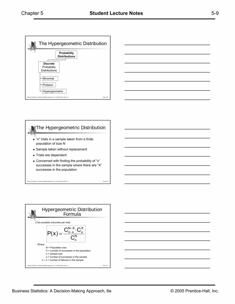
The Hypergeometric Distribution
“n” trials in a sample taken from a finite population of size N
Sample taken without replacement
Trials are dependent
Concerned with finding the probability of “x” successes in the sample where there are “X” successes in the population
Business Statistics: A Decision-Making Approach, 6e © 2005 Prentice-Hall, Inc. Chap 5-27
Hypergeometric Distribution Formula
Nn
Xx
XNxn
CCC)x(P
−−=
.
WhereN = Population sizeX = number of successes in the populationn = sample sizex = number of successes in the sample
n – x = number of failures in the sample
(Two possible outcomes per trial)

Business Statistics: A Decision-Making Approach, 6e © 2005 Prentice-Hall, Inc.
Chapter 5 Student Lecture Notes 5-10
Business Statistics: A Decision-Making Approach, 6e © 2005 Prentice-Hall, Inc. Chap 5-28
Hypergeometric Distribution Formula
0.3120
(6)(6)C
CCC
CC2)P(x 103
42
61
Nn
Xx
XNxn =====
−−
■ Example: 3 Light bulbs were selected from 10. Of the 10 there were 4 defective. What is the probability that 2 of the 3 selected are defective?
N = 10 n = 3X = 4 x = 2
Business Statistics: A Decision-Making Approach, 6e © 2005 Prentice-Hall, Inc. Chap 5-29
Hypergeometric Distribution in PHStat
Select:PHStat / Probability & Prob. Distributions / Hypergeometric …
Business Statistics: A Decision-Making Approach, 6e © 2005 Prentice-Hall, Inc. Chap 5-30
Hypergeometric Distribution in PHStat
Complete dialog box entries and get output …
N = 10 n = 3X = 4 x = 2
P(x = 2) = 0.3
(continued)
Business Statistics: A Decision-Making Approach, 6e © 2005 Prentice-Hall, Inc.
Chapter 5 Student Lecture Notes 5-11
Business Statistics: A Decision-Making Approach, 6e © 2005 Prentice-Hall, Inc. Chap 5-31
The Normal Distribution
ContinuousProbability
Distributions
Probability Distributions
Normal
Uniform
Exponential
Business Statistics: A Decision-Making Approach, 6e © 2005 Prentice-Hall, Inc. Chap 5-32
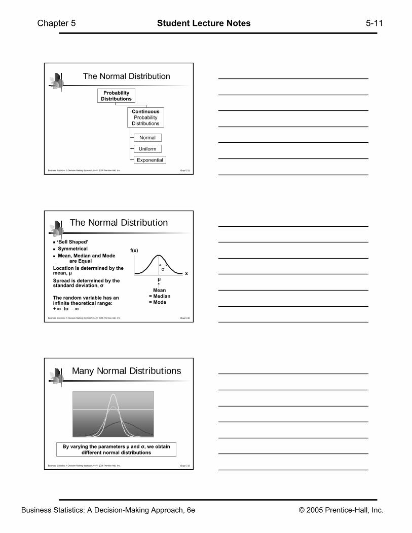
The Normal Distribution
‘Bell Shaped’SymmetricalMean, Median and Mode
are EqualLocation is determined by the mean, µSpread is determined by the standard deviation, σ
The random variable has an infinite theoretical range: + ∞ to − ∞
Mean = Median = Mode
x
f(x)
µ
σ
Business Statistics: A Decision-Making Approach, 6e © 2005 Prentice-Hall, Inc. Chap 5-33
By varying the parameters µ and σ, we obtain different normal distributions
Many Normal Distributions
Business Statistics: A Decision-Making Approach, 6e © 2005 Prentice-Hall, Inc.
Chapter 5 Student Lecture Notes 5-12
Business Statistics: A Decision-Making Approach, 6e © 2005 Prentice-Hall, Inc. Chap 5-34
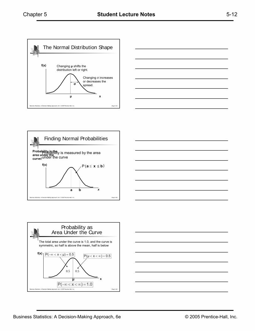
The Normal Distribution Shape
x
f(x)
µ
σ
Changing µ shifts the distribution left or right.
Changing σ increases or decreases the spread.
Business Statistics: A Decision-Making Approach, 6e © 2005 Prentice-Hall, Inc. Chap 5-35
Finding Normal Probabilities
Probability is the area under thecurve!
a b x
f(x) P a x b( )≤ ≤
Probability is measured by the area under the curve
Business Statistics: A Decision-Making Approach, 6e © 2005 Prentice-Hall, Inc. Chap 5-36
f(x)
xµ
Probability as Area Under the Curve
0.50.5
The total area under the curve is 1.0, and the curve is symmetric, so half is above the mean, half is below
1.0)xP( =∞<<−∞
0.5)xP(µ =∞<<0.5µ)xP( =<<−∞
Business Statistics: A Decision-Making Approach, 6e © 2005 Prentice-Hall, Inc.
Chapter 5 Student Lecture Notes 5-13
Business Statistics: A Decision-Making Approach, 6e © 2005 Prentice-Hall, Inc. Chap 5-37
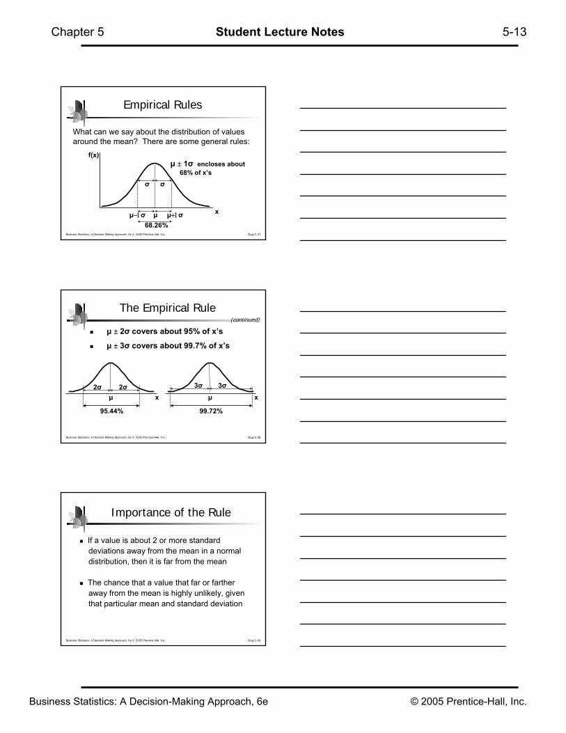
Empirical Rules
µ ± 1σ encloses about 68% of x’s
f(x)
xµ µ+1σµ−1σ
What can we say about the distribution of values around the mean? There are some general rules:
σσ
68.26%
Business Statistics: A Decision-Making Approach, 6e © 2005 Prentice-Hall, Inc. Chap 5-38
The Empirical Rule
µ ± 2σ covers about 95% of x’s
µ ± 3σ covers about 99.7% of x’s
xµ2σ 2σ
xµ3σ 3σ
95.44% 99.72%
(continued)
Business Statistics: A Decision-Making Approach, 6e © 2005 Prentice-Hall, Inc. Chap 5-39
Importance of the Rule
If a value is about 2 or more standarddeviations away from the mean in a normaldistribution, then it is far from the mean
The chance that a value that far or farther away from the mean is highly unlikely, giventhat particular mean and standard deviation

Business Statistics: A Decision-Making Approach, 6e © 2005 Prentice-Hall, Inc.
Chapter 5 Student Lecture Notes 5-14
Business Statistics: A Decision-Making Approach, 6e © 2005 Prentice-Hall, Inc. Chap 5-40
The Standard Normal Distribution
Also known as the “z” distributionMean is defined to be 0Standard Deviation is 1
z
f(z)
0
1
Values above the mean have positive z-values, values below the mean have negative z-values
Business Statistics: A Decision-Making Approach, 6e © 2005 Prentice-Hall, Inc. Chap 5-41
The Standard Normal
Any normal distribution (with any mean and standard deviation combination) can be transformed into the standard normaldistribution (z)
Need to transform x units into z units
Business Statistics: A Decision-Making Approach, 6e © 2005 Prentice-Hall, Inc. Chap 5-42
Translation to the Standard Normal Distribution
Translate from x to the standard normal (the “z” distribution) by subtracting the mean of x and dividing by its standard deviation:
σµxz −
=
Business Statistics: A Decision-Making Approach, 6e © 2005 Prentice-Hall, Inc.
Chapter 5 Student Lecture Notes 5-15
Business Statistics: A Decision-Making Approach, 6e © 2005 Prentice-Hall, Inc. Chap 5-43
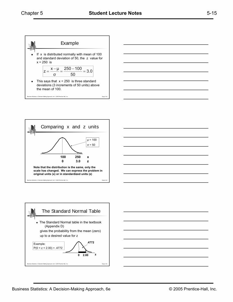
Example
If x is distributed normally with mean of 100and standard deviation of 50, the z value for x = 250 is
This says that x = 250 is three standard deviations (3 increments of 50 units) above the mean of 100.
3.050
100250σ
µxz =−
=−
=
Business Statistics: A Decision-Making Approach, 6e © 2005 Prentice-Hall, Inc. Chap 5-44
Comparing x and z units
z100
3.00250 x
Note that the distribution is the same, only the scale has changed. We can express the problem in original units (x) or in standardized units (z)
µ = 100
σ = 50
Business Statistics: A Decision-Making Approach, 6e © 2005 Prentice-Hall, Inc. Chap 5-45
The Standard Normal Table
The Standard Normal table in the textbook (Appendix D)
gives the probability from the mean (zero)up to a desired value for z
z0 2.00
.4772Example:P(0 < z < 2.00) = .4772
Business Statistics: A Decision-Making Approach, 6e © 2005 Prentice-Hall, Inc.
Chapter 5 Student Lecture Notes 5-16
Business Statistics: A Decision-Making Approach, 6e © 2005 Prentice-Hall, Inc. Chap 5-46
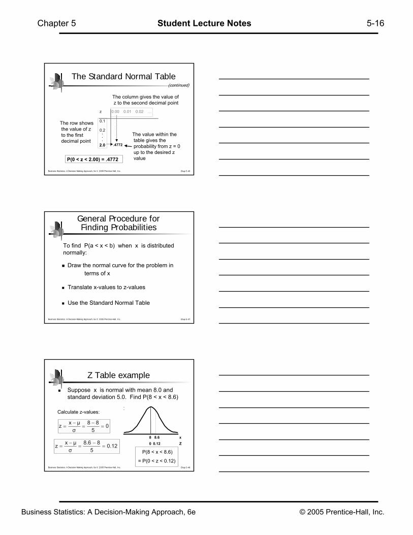
The Standard Normal Table
The value within the table gives the probability from z = 0up to the desired z value
z 0.00 0.01 0.02 …
0.1
0.2
.4772
2.0P(0 < z < 2.00) = .4772
The row shows the value of z to the first decimal point
The column gives the value of z to the second decimal point
2.0
.
..
(continued)
Business Statistics: A Decision-Making Approach, 6e © 2005 Prentice-Hall, Inc. Chap 5-47
General Procedure for Finding Probabilities
Draw the normal curve for the problem interms of x
Translate x-values to z-values
Use the Standard Normal Table
To find P(a < x < b) when x is distributed normally:
Business Statistics: A Decision-Making Approach, 6e © 2005 Prentice-Hall, Inc. Chap 5-48
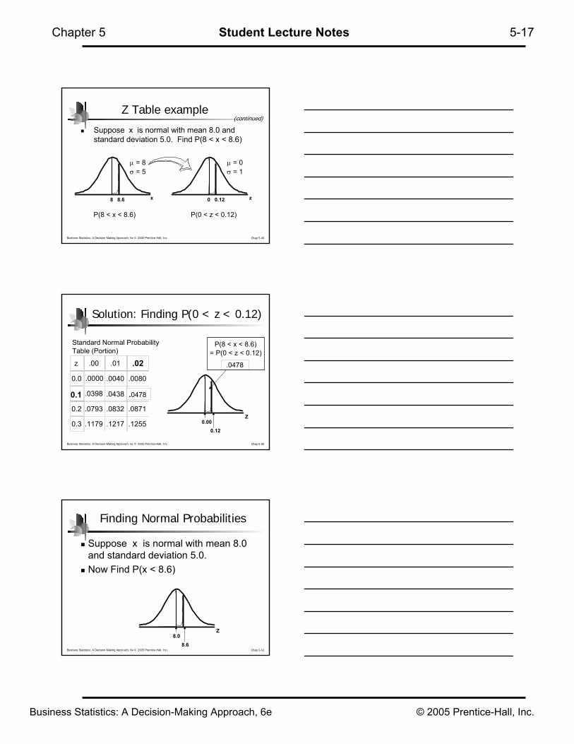
Z Table example
Suppose x is normal with mean 8.0 and standard deviation 5.0. Find P(8 < x < 8.6)
P(8 < x < 8.6)
= P(0 < z < 0.12)
Z0.120x8.68
05
88σ
µxz =−
=−
=
0.125
88.6σ
µxz =−
=−
=
Calculate z-values:
Business Statistics: A Decision-Making Approach, 6e © 2005 Prentice-Hall, Inc.
Chapter 5 Student Lecture Notes 5-17
Business Statistics: A Decision-Making Approach, 6e © 2005 Prentice-Hall, Inc. Chap 5-49
Z Table example
Suppose x is normal with mean 8.0 and standard deviation 5.0. Find P(8 < x < 8.6)
P(0 < z < 0.12)
z0.120x8.68
P(8 < x < 8.6)
µ = 8σ = 5
µ = 0σ = 1
(continued)
Business Statistics: A Decision-Making Approach, 6e © 2005 Prentice-Hall, Inc. Chap 5-50
Z
0.12
z .00 .01
0.0 .0000 .0040 .0080
.0398 .0438
0.2 .0793 .0832 .0871
0.3 .1179 .1217 .1255
Solution: Finding P(0 < z < 0.12)
.0478.02
0.1 .0478
Standard Normal Probability Table (Portion)
0.00
= P(0 < z < 0.12)P(8 < x < 8.6)
Business Statistics: A Decision-Making Approach, 6e © 2005 Prentice-Hall, Inc. Chap 5-51
Finding Normal Probabilities
Suppose x is normal with mean 8.0 and standard deviation 5.0. Now Find P(x < 8.6)
Z
8.68.0
Business Statistics: A Decision-Making Approach, 6e © 2005 Prentice-Hall, Inc.
Chapter 5 Student Lecture Notes 5-18
Business Statistics: A Decision-Making Approach, 6e © 2005 Prentice-Hall, Inc. Chap 5-52
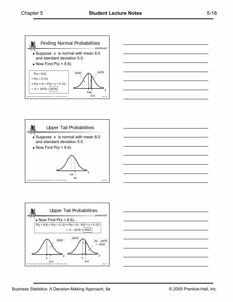
Finding Normal Probabilities
Suppose x is normal with mean 8.0 and standard deviation 5.0. Now Find P(x < 8.6)
(continued)
Z
0.12
.0478
0.00
.5000P(x < 8.6)
= P(z < 0.12)
= P(z < 0) + P(0 < z < 0.12)
= .5 + .0478 = .5478
Business Statistics: A Decision-Making Approach, 6e © 2005 Prentice-Hall, Inc. Chap 5-53
Upper Tail Probabilities
Suppose x is normal with mean 8.0 and standard deviation 5.0. Now Find P(x > 8.6)
Z
8.68.0
Business Statistics: A Decision-Making Approach, 6e © 2005 Prentice-Hall, Inc. Chap 5-54
Now Find P(x > 8.6)…(continued)
Z
0.120
Z
0.12
.0478
0
.5000 .50 - .0478 = .4522
P(x > 8.6) = P(z > 0.12) = P(z > 0) - P(0 < z < 0.12)
= .5 - .0478 = .4522
Upper Tail Probabilities

Business Statistics: A Decision-Making Approach, 6e © 2005 Prentice-Hall, Inc.
Chapter 5 Student Lecture Notes 5-19
Business Statistics: A Decision-Making Approach, 6e © 2005 Prentice-Hall, Inc. Chap 5-55
Lower Tail Probabilities
Suppose x is normal with mean 8.0 and standard deviation 5.0. Now Find P(7.4 < x < 8)
Z
7.48.0
Business Statistics: A Decision-Making Approach, 6e © 2005 Prentice-Hall, Inc. Chap 5-56
Lower Tail Probabilities
Now Find P(7.4 < x < 8)…
Z
7.48.0
The Normal distribution is symmetric, so we use the same table even if z-values are negative:
P(7.4 < x < 8)
= P(-0.12 < z < 0)
= .0478
(continued)
.0478
Business Statistics: A Decision-Making Approach, 6e © 2005 Prentice-Hall, Inc. Chap 5-57
Normal Probabilities in PHStat
We can use Excel and PHStat to quicklygenerate probabilities for any normaldistribution
We will find P(8 < x < 8.6) when x isnormally distributed with mean 8 andstandard deviation 5
Business Statistics: A Decision-Making Approach, 6e © 2005 Prentice-Hall, Inc.
Chapter 5 Student Lecture Notes 5-20
Business Statistics: A Decision-Making Approach, 6e © 2005 Prentice-Hall, Inc. Chap 5-58
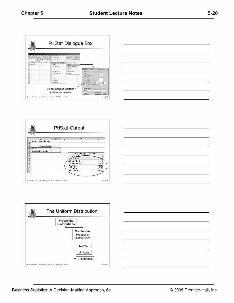
PHStat Dialogue Box
Select desired options and enter values
Business Statistics: A Decision-Making Approach, 6e © 2005 Prentice-Hall, Inc. Chap 5-59
PHStat Output
Business Statistics: A Decision-Making Approach, 6e © 2005 Prentice-Hall, Inc. Chap 5-60
The Uniform Distribution
ContinuousProbability
Distributions
Probability Distributions
Normal
Uniform
Exponential
Business Statistics: A Decision-Making Approach, 6e © 2005 Prentice-Hall, Inc.
Chapter 5 Student Lecture Notes 5-21
Business Statistics: A Decision-Making Approach, 6e © 2005 Prentice-Hall, Inc. Chap 5-61
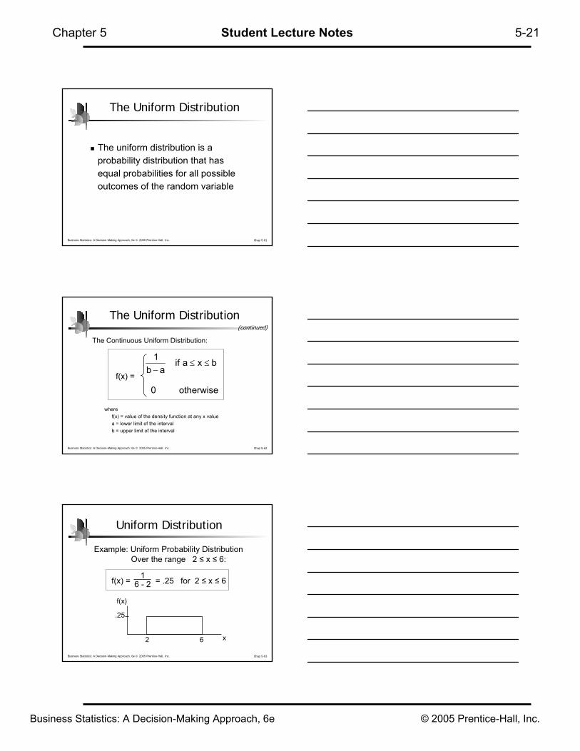
The Uniform Distribution
The uniform distribution is a probability distribution that has equal probabilities for all possible outcomes of the random variable
Business Statistics: A Decision-Making Approach, 6e © 2005 Prentice-Hall, Inc. Chap 5-62
The Continuous Uniform Distribution:
otherwise 0
bxaifab
1≤≤
−
wheref(x) = value of the density function at any x valuea = lower limit of the intervalb = upper limit of the interval
The Uniform Distribution(continued)
f(x) =
Business Statistics: A Decision-Making Approach, 6e © 2005 Prentice-Hall, Inc. Chap 5-63
Uniform Distribution
Example: Uniform Probability DistributionOver the range 2 ≤ x ≤ 6:
2 6
.25
f(x) = = .25 for 2 ≤ x ≤ 66 - 21
x
f(x)
Business Statistics: A Decision-Making Approach, 6e © 2005 Prentice-Hall, Inc.
Chapter 5 Student Lecture Notes 5-22
Business Statistics: A Decision-Making Approach, 6e © 2005 Prentice-Hall, Inc. Chap 5-64
The Exponential Distribution
ContinuousProbability
Distributions
Probability Distributions
Normal
Uniform
Exponential
Business Statistics: A Decision-Making Approach, 6e © 2005 Prentice-Hall, Inc. Chap 5-65
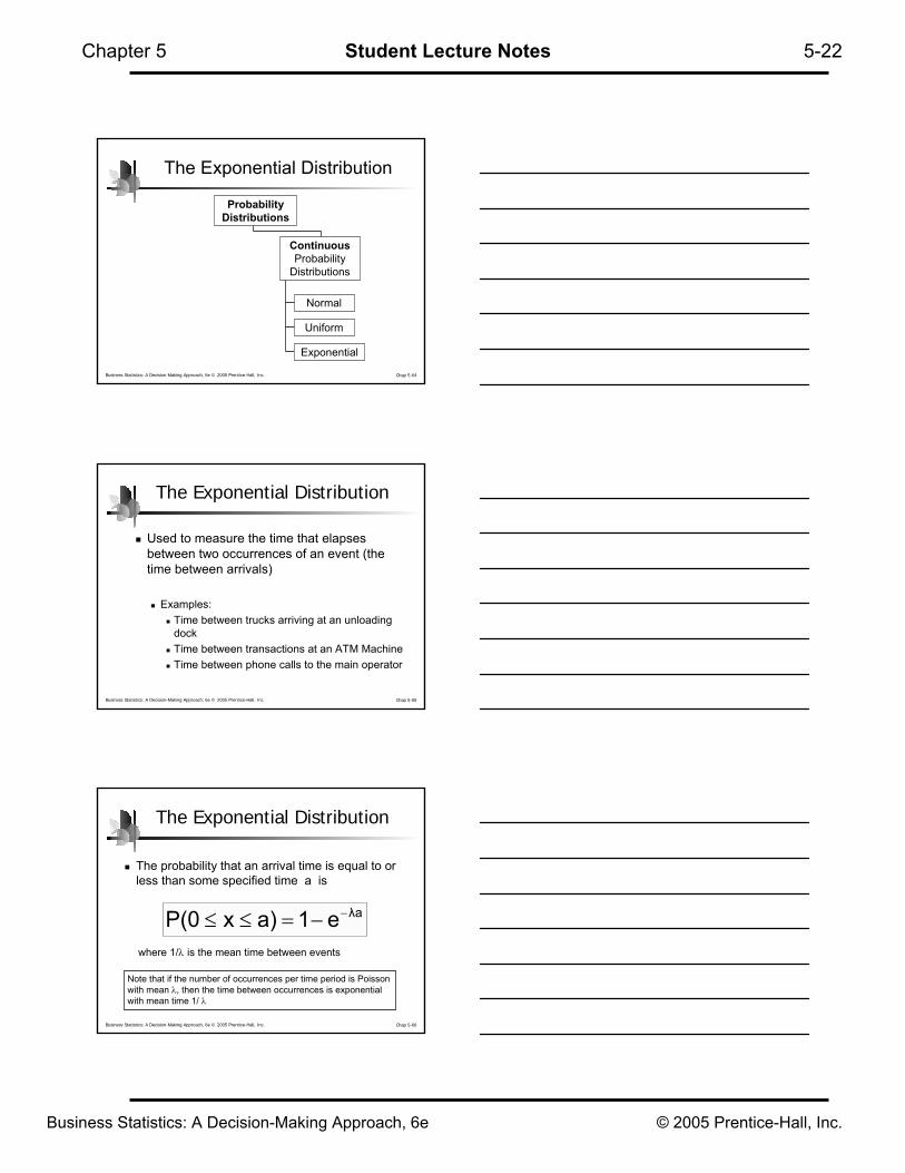
The Exponential Distribution
Used to measure the time that elapses between two occurrences of an event (the time between arrivals)
Examples: Time between trucks arriving at an unloading dockTime between transactions at an ATM MachineTime between phone calls to the main operator
Business Statistics: A Decision-Making Approach, 6e © 2005 Prentice-Hall, Inc. Chap 5-66
The Exponential Distribution
aλe1a)xP(0 −−=≤≤
The probability that an arrival time is equal to or less than some specified time a is
where 1/λ is the mean time between events
Note that if the number of occurrences per time period is Poisson with mean λ, then the time between occurrences is exponential with mean time 1/ λ
Business Statistics: A Decision-Making Approach, 6e © 2005 Prentice-Hall, Inc.
Chapter 5 Student Lecture Notes 5-23
Business Statistics: A Decision-Making Approach, 6e © 2005 Prentice-Hall, Inc. Chap 5-67
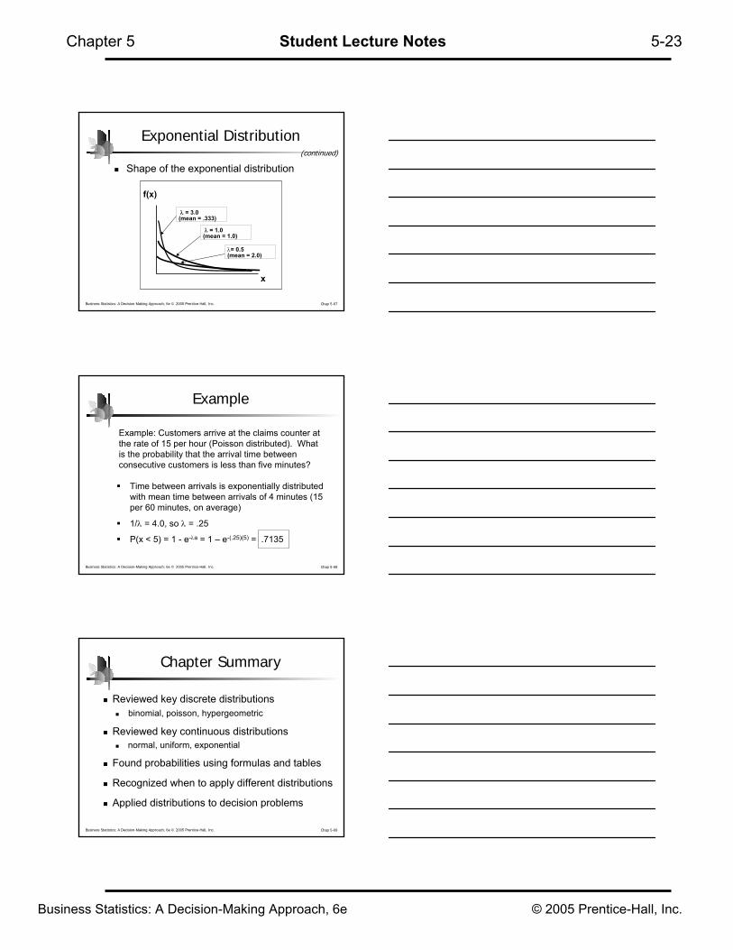
Exponential Distribution
Shape of the exponential distribution(continued)
f(x)
x
λ = 1.0(mean = 1.0)
λ= 0.5 (mean = 2.0)
λ = 3.0(mean = .333)
Business Statistics: A Decision-Making Approach, 6e © 2005 Prentice-Hall, Inc. Chap 5-68
Example
Example: Customers arrive at the claims counter at the rate of 15 per hour (Poisson distributed). What is the probability that the arrival time between consecutive customers is less than five minutes?
Time between arrivals is exponentially distributed with mean time between arrivals of 4 minutes (15 per 60 minutes, on average)
1/λ = 4.0, so λ = .25
P(x < 5) = 1 - e-λa = 1 – e-(.25)(5) = .7135
Business Statistics: A Decision-Making Approach, 6e © 2005 Prentice-Hall, Inc. Chap 5-69
Chapter Summary
Reviewed key discrete distributionsbinomial, poisson, hypergeometric
Reviewed key continuous distributionsnormal, uniform, exponential
Found probabilities using formulas and tables
Recognized when to apply different distributions
Applied distributions to decision problems