chapter 5 stewart 8e - new river community college

Chapter 5 Notes, Stewart 8e Chalmeta

Contents

5.1 Areas and Distances . . . . . . . . . . . . . . . . . . . . . . . . . . . . . . . . . . . . . . . . 2 5.1.1 Area . . . . . . . . . . . . . . . . . . . . . . . . . . . . . . . . . . . . . . . . . . . . . 2 5.1.2 Distance . . . . . . . . . . . . . . . . . . . . . . . . . . . . . . . . . . . . . . . . . . . 6

5.2 The Definite Integral . . . . . . . . . . . . . . . . . . . . . . . . . . . . . . . . . . . . . . . . 8 5.2.1 Riemann Sums . . . . . . . . . . . . . . . . . . . . . . . . . . . . . . . . . . . . . . . 8 5.2.2 The Definite Integral . . . . . . . . . . . . . . . . . . . . . . . . . . . . . . . . . . . . 9 5.2.3 Evaluating Definite Integrals . . . . . . . . . . . . . . . . . . . . . . . . . . . . . . . 10

5.3 The Fundamental Theorem of Calculus . . . . . . . . . . . . . . . . . . . . . . . . . . . . . . 16 5.3.1 The Fundamental Theorem of Calculus, Part I . . . . . . . . . . . . . . . . . . . . . 16 5.3.2 The Fundamental Theorem of Calculus, Part II . . . . . . . . . . . . . . . . . . . . . 18

5.4 Indefinite Integrals . . . . . . . . . . . . . . . . . . . . . . . . . . . . . . . . . . . . . . . . . 20 5.5 The Substitution Rule . . . . . . . . . . . . . . . . . . . . . . . . . . . . . . . . . . . . . . . 24

5.5.1 U-Substitution for Indefinite Integrals . . . . . . . . . . . . . . . . . . . . . . . . . . 24 5.5.2 U-Substitution for Definite Integrals . . . . . . . . . . . . . . . . . . . . . . . . . . . 27 5.5.3 Double U substitution . . . . . . . . . . . . . . . . . . . . . . . . . . . . . . . . . . . 29

1


5.1 Areas and Distances

5.1.1 Area

Consider the problem of finding the area under the curve on the function y −x2 + 5 over the domain [0, 2]. We can approximate this area by using a familiar shape, the rectangle. If we divide the domain interval into several pieces, then draw rectangles having the width of the pieces, and the height of the curve, we can get a rough idea of the total area.

For example suppose we divide the interval [0, 2] into 5 equal subintervals of length

∆x b − a n

, i.e., each of width 2 5 .

The intervals are [0 , 0.4], [0.4 , 0.8], [0.8 , 1.2], [1.2 , 1.6], [1.6 , 2.0]. The table below shows the values obtained when y (x) is evaluated at the corresponding points.

x y −x2 + 5

0 5

0.4 4.84

0.8 4.36

1.2 3.56

1.6 2.44

2 1

Plotting these points yields the following graph.

0

1

2

3

4

5

0 1 2 x

y

y −x2 + 5

If we find the minimum value in the subinterval, and use this as our height for that rectangle, we have what is known as an inscribed rectangle. See the graph below.

0

1

2

3

4

5

0 1 2

=

=

=

=

y

y = −x2 + 5

x

Now each of the above rectangles has the exact same width, namely 2/5. For this function the height of each rectangle is given by calculating the value of the function at the right hand endpoint of each subinterval. The area under the curve, can then be approximated by adding the areas of all the rectangles together.

2


Notice that when using the minimum values, i.e. using inscribed rectangles, we arrive at an estimate that is lower than the actual area under the curve. Hence, this method results in what is known as the lower sum or an underestimate. Let’s calculate this estimate using the right endpoints

R5

5∑

i=1

F (xi) ∆xi

f

(2 5

) 2 5 + f

(4 5

) 2 5 + f

(6 5

) 2 5 + f

(8 5

) 2 5 + f (2)

2 5

2 5

[f

(2 5

)

+ f

(4 5

)

+ f

(6 5

)

+ f

(8 5

)

+ f (2)

]

2 5 [4.84 + 4.36 + 3.56 + 2.44 + 1]

2 5 [16.2]

6.48

You can also calculate an estimate using the maximum value in the subinterval and using it as the height of the rectangles. These rectangles are known as circumscribed rectangles. The resulting area approximation will be greater than the area under the curve. Consequently, we call this type of sum an upper sum or an oversetimate.

0 1 2 3 4 5

0 1 2

= ·

=

=

=

=

=

y

y = −x2 + 5

x

Calculuating the sum with the left endpoints we get:

5∑ L5 = F (xi−1) · ∆xi

i=1 ( ) ( ) ( ) ( ) 2 2 2 4 2 6 2 8 2

= f (0) + f + f + f + f 5 5 5 5 5 5 5 5 5 [ ( ) ( ) ( ) ( )]

2 2 4 6 8 = f (0) + f + f + f + f

5 5 5 5 5

2 = [5 + 4.84 + 4.36 + 3.56 + 2.44]

5 2

= [20.2] 5

= 8.08

From the two calculations above we can conclude that the area of the curve lies some where between the two approximations, i.e. 6.48 < area of region < 8.08

3


Another method that can yield a better approximation is known as the midpoint rule. In the midpoint rule, you choose the value exactly in the middle of the subinterval to use in calculating the height of the rectangle; resulting in some rectangles being both inscribed and circumscribed.

0

1

2

3

4

5

0 1 2 x

y

y −x2 + 5

Let’s calculate the above estimate: The Midpoint Sum.

M5

5∑

i=1

F (x ∗ i ) ∆x

f

(1 5

) 2 5 + f

(3 5

) 2 5 + f

(5 5

) 2 5 + f

(7 5

) 2 5 + f

(9 5

) 2 5

2 5

[f

(1 5

)

+ f

(3 5

)

+ f

(5 5

)

+ f

(7 5

)

+ f

(9 5

)]

2 5 [4.96 + 4.64 + 4 + 3.04 + 1.76]

2 5 [18.4]

7.36

NOTE: The smaller the subintervals, the better the approximation will be. This is because, the function’s values

are changing less in the subinterval, i.e. the value of the function is fairly constant in each subinterval. Consequently, we are not approximating by such a rough amount each time. For example, here is the same region divided into 20 rectangle instead of 5. Note that the error is minute compared with the previous work.

0

1

2

3

4

5

0 1 2

-

=

= ·

=

=

=

=

=

y

y = −x2 + 5

x

a. Each of the above processes (lower sum, upper sum, midpoint sum) are just approximations. They are not exact.

b. When you want to calculate the Volume of a solid, you can use similar techniques, only you’ll be using rectangular solids or cylinders to approximate the volume.

4


Definition 5.1. The area A of the region S that lies under the graph of the continuous function f(x) is the limit of the sum of the areas of approximating rectangles:

n∑ A = lim Rn = lim f(xi) · ∆x = lim [f(x1)∆x + f(x2)∆x + · · · + f(xn)∆x] ,

n→∞ n→∞ n→∞ i=1

b − a where ∆x = , xi = a +∆x · i.

n

Example 5.1.1. Use definition 5.1 to find an expression for the exact area under the given curves on the indicated intervals.

1. f(x) = −x2 + 5 on [0, 2].

√ 2. f(x) = x on [1, 4].

Accuracy:

Error Magnitude = |true value - calculated value|

|true value − calculated sum| Relative Error =

true value

|true value−calculated sum| Percentage Error = (100%) true value

For the example in part I, the true value for the area under the curve y = −x2 + 5 over the domain [0, 2] is 22 = 7.33. Therefore the error associated with the approximations are: 3

| 22 −6.48| 3

22 ≈ 0.11636364 Errorlower sum = 3

| 22 −8.08| Errorupper sum = 3

22 ≈ 0.1018182 3

| 22 −6.48| = 3

22 ≈ 0.0036364 Errormidpoint sum 3

5


5.1.2 Distance

A. Constant Velocity

If the velocity of an object remains constant, then the distance can be computed by

distance = velocity × time

B. Variable velocity

1. If the velocity varies, i.e., the object moves with velocity, v = f(t) where a ≤ t ≤ b and f(t) ≥ 0, then we will think of the velocity as a constant on each subinterval. If the times are equally spaced,

b − a then ∆t = .

n n∑

Using the left endpoints, the total distance= f(ti−1) · ∆t. i=1

n∑ Using the right endpoints, the total distance= f(ti) · ∆t.

i=1

n∑ ∗ Using the midpoints, the total distance= f(t i ) · ∆t.

i=1

2. This can be thought of as finding the area under the velocity curve where the base of the rectangle b − a

is ∆t = and the height of the rectangle is v = f(t). n

n n∑ ∑ 3. Definition: distance = A = lim f(ti−1) · ∆t = lim f(ti) · ∆t

n→∞ n→∞ i=1 i=1

Example 5.1.2. A radar gun was used to record the speed of a runner at the times in the table. Estimate the distance the runner covered during those 5 seconds.

t (s) v (m/s) t (s) v (m/s)

0 0 3.0 10.5 0.5 4.67 3.5 10.67 1.0 7.34 4.0 10.76 1.5 8.86 4.5 10.81 2.0 9.73 5.0 10.81 2.5 10.22

Using left hand endpoints:

6


Using right hand endpoints:

Using midpoints:

Example 5.1.3. Uneven Subintervals: Given y = x3 on [1, 3]. Use the table below to estimate the area between the curve and the x-axis

using the left endpoints.

3 x y = x

1 1 1.4 2.744 1.6 4.096 2.1 9.261 2.2 10.648 2.5 15.625 3 27

Example 5.1.4. If the function is not strictly increasing nor decreasing. The table below gives the velocity at the specified time. Use this data to give an estimation of the

distance traveled.

time (s) 0 2 4 6 8 10

velocity (ft/s) 0 6.1 12.5 8.3 4.9 0

7


5.2 The Definite Integral

5.2.1 Riemann Sums

Definition 5.2. Given y = f(x): 1. Let f(x) be defined on a closed interval [a,b]. 2. Partition [a,b] into n subintervals [xi−1, xi] of length ∆xi = xi − xi−1. Let P denote the partition

a = x0 < x1 < x2 < · · · < xn−1 < xn = b. 3. Let ||P || be the length of the longest subinterval. (||P || - norm of the partition P .)

∗ ∗ 4. Choose a number x i in each subinterval ( x i may be an endpt). ∑ ∗ 5. Form the Riemann Sum = SP = [f (x i )] (∆xi)

NOTES:

1. f(x) does not have to be continuous nor nonnegative on [a,b]. Therefore, SP does not necessarily represent an approximation to the area under a graph.

∗ 2. x need not be the same in each interval. i

3. ∆xi need not be the same length.

4. Riemann Sums are used to approximate a given quantity.

5. To increase the accuracy of the sum, decrease the subinterval length; hence, increase the number of subintervals.

6. As the accuracy of the sum increases, Riemann Sum −→ Definite Integral.

Example 5.2.1. Finite Sums are an example of Riemann Sums in which each subinterval has the same ∗ length and the same x i is chosen for each subinterval.

Example 5.2.2. 2. Given y = x2 on [1,2]. Partition [1,2] into the 4 subintervals: [1, 1.3], [1.3, 1.5], [1.5,1.6] & [1.6,2]. Let x1 =1, x2 =1.4, x3 =1.6, x4 =1.9. Find the Riemann Sum using this information.

Example 5.2.3. Repeat using 4 equal subintervals and xi being the midpoint of each subinterval.

8


5.2.2 The Definite Integral

Definition 5.3. If f(x) is a continuous function defined for a ≤ x ≤ b, we divide the interval [a, b] b − a

into n subintervals of equal width ∆x = . We let x0(= a), x1, x2, · · · , xn(= b) be the endpoints of n

∗ ∗ ∗ ∗ these subintervals and we choose sample points x 1, x 2, · · · , x n in these subintervals, so x lies in the ith i

subinterval [xi−1, xi]. Then the definite integral of f(x) from a to b is ∫ b n∑ ∗ f(x) dx = lim [f (x i )] (∆x).

n→∞ a i=1

NOTE: ∫ b

1. The definite integral f(x) dx is a number; it does not depend on x. a ∫ b ∫ b ∫ b

f(x) dx = f(t) dt = f(r) dr a a a

2. Because we have assumed that f(x) is continuous, it can be proved that the limit in the definition ∗ always exists and gives the same value no matter how the sample points x i have been chosen. ∫ b

3. f(x) dx gives the signed area of a region between the curve y = f(x) and the x-axis on [a, b]. a

Theorem: All continuous functions are integrable, i.e., if a function f(x) is continuous on [a, b], then its definite integral over [a, b] exists.

Example 5.2.4. Express the limit as a definite integral on the given interval

n∑ a. lim (6xi − 3xi ) (∆x); [-2, 3]

n→∞ i=1

n∑( )5 b. lim (xi)

3 − 7 (∆x); [4, 7] n→∞

i=1

√ n ( )2 ( ) ∑ 4i 4

c. lim 3 2 − 1 + =

n→∞ n ni=1

9

4

1


Example 5.2.5. Express the definite integrals as a limit: ∫ b n∑ ∗ f(x) dx = lim f (x i )∆x

n→∞ a i=1

b − a ∗ ∗ where ∆x = and x i is the right hand endpoint , i.e., x i = a + (∆x)i. n

∫ 9

a. (x 2 − 2x + 3) dx

∫ 4

b. (x 3 + x) dx

5.2.3 Evaluating Definite Integrals

A. Approximating the Value of Definite Integrals

n∑ ∗ In the previous section we used the area of rectangles [f (x i )] (∆x) to approximate the area under

i=1 a curve. We now know that the definite integral gives us the ”signed” area between a curve and the x-axis. Therefore, we can use this method to approximate the definite integral. If we use midpoints as

∗ the x i value in the definition of a Riemann sum, we call it the Midpoint Rule:

∫ b n∑ f(x) dx = [f (x̄i)] (∆x) = ∆x [f (x̄1) + f (x̄2) + · · · + f (x̄n)]

a i=1

b−a 1 where ∆x = n and x̄i = 2 (xi−1 + xi)= midpoint of [xi−1, xi]. ∫ 2 1 Example 5.2.6. Use the Midpoints Rule with n = 5 to approximate dx

x 1

10


B. Evaluating the Exact Value of a Definite Integral.

Example 5.2.7. Using geometry / area of a region to evaluate the exact value of a definite integral Sometimes the only way to evaluate a definite integral is to use geometry, as in the first example.

1) ∫ 5

−5

√ 25 − x2 dx

2) ∫ 5

0 (2 − x)dx

3) Use the graph of g(x) below to evaluate ∫ 5

0 g(x) dx

0

1

2

−1

−2

1 2 3 4 5

y

g(x)

x

n∑ Example 5.2.8. Given that sigma notation for finite sums is ak = a1 + a2 + a3 + · · · + an, evaluate

k=1 the following.

4 ( ) ∑ i 1) =

3i=1

∑ 2) (3j + 1) =

j=−2

11

3


C. Sum Formulas for Positive Integers

n n∑ ∑ (a) 1 = n; c = c · n; where c is a constant.

i=1 i=1

n∑ n(n + 1) (b) i =

2 i=1

(c) n∑

i2 = n(n + 1)(2n + 1)

6 i=1

(d) n∑

i3

i=1

=

[ ]2 n(n + 1) 2

D. Algebra Rules for Finite Sums

n n n∑ ∑ ∑ (a) Sum/Difference Rule: (ak ± bk) = (ak) ± (bk)

k=1 k=1 k=1

n n∑ ∑ (b) Constant Multiple Rule: c · ak = c ak, where c is a constant.

k=1 k=1

Example 5.2.9. Evaluate the following

10∑ 1) k2 − 3k + 2

k=1

20∑ 2) 4k2

k=5

12


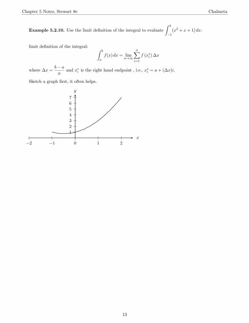
Example 5.2.10. Use the limit definition of the integral to evaluate ∫ 2

−1 (x 2 + x + 1) dx.

limit definition of the integral: ∫ b

a f(x) dx lim

n→∞

n∑

i=1

f (x ∗ i ) ∆x

where ∆x b − a n

and x ∗ i is the right hand endpoint , i.e., x ∗

i a + (∆x)i.

Sketch a graph first, it often helps.

1 2 3 4 5 6 7

0 1 2 −1 −2

=

= =

y

x

13


E. Properties of the definite integrals

∫ a ∫ b ∫ a

a. f(x) dx = 0 b. f(x) dx = − f(x) dx = 0 a a b ∫ b ∫ b ∫ b

c. c dx = c(b − a); c = constant function. d. c · f(x) dx = c f(x) dx a a a ∫ b ∫ b ∫ b

e. f(x) ± g(x) dx = f(x) dx ± g(x) dx a a a ∫ c ∫ b ∫ b

f. f(x) dx + f(x) dx = f(x) dx a c a

∫ 1 ∫ 3 ∫ 2 ∫ 3

Example 5.2.11. Given that f(x) dx = 7, f(x) dx = 5, g(x) dx = 3, and g(x) dx = −8, −2 1 −2 2

evaluate the following: ∫ 1

1) f(x) dx = 3

∫ 3

2) f(x) dx = −2

∫ 2

3) −6g(x) dx = −2

∫ 3

4) [2f(x) + 4g(x)] dx = −2

∫ 2

5) 5 dx = −1

14


F. Comparison properties of the integrals ∫ b

(a) If f(x) ≥ 0 on [a, b] then f(x) dx ≥ 0. a ∫ b ∫ b

(b) If f(x) ≥ g(x) on [a, b] then f(x) dx ≥ g(x) dx. a a

(c) Max-Min inequality: If M and m are the maximum and the minimum values of f(x) on [a, b] then ∫ b

m(b − a) ≤ f(x) dx ≤ M(b − a). a

∫ 2

Example 5.2.12. Show that the value of sin(x 2) dx can not be 4. 0

15


5.3 The Fundamental Theorem of Calculus

5.3.1 The Fundamental Theorem of Calculus, Part I

Fundamental Theorem 1: If f(x) is continuous on [a, b], then the function g(x) defined by ∫ x

g(x) = f(t) dt; a ≤ x ≤ b a

is continuous on [a, b] and differentiable on (a, b), and [∫ ] x

g ′ (x) = d

f(t) dt = f(x); a ≤ x ≤ b dx a

Extension of Theorem: [∫ ] u(x) d

f(t) dt = f(u(x))u ′ (x); a ≤ x ≤ b dx a

Example 5.3.1. Find the following derivatives. [∫ ] x d 1) sin(t) dt =

dx −π

[∫ ] x d dr 2) =

dx r 1

[∫ 2 ]

3) d

5x 2 dx = dy y

[∫ ] 3 xd

4) tan(t) dt = dx 0

∫ t Example 5.3.2. If f(t) = (x 2 + 1) dx, find f ′ (0).

0

∫ 3x dt y Example 5.3.3. Let y = . Find d2

dx2 . 1 t2 + t + 1

16


Example 5.3.4. Let f(x) ∫ x

−3 g(t) dt where g(x) is the function whose graph is shown below. Then

answer the following.

1

2

−1

−2

1 2 3 4 5 −1 −2 −3 −4 x

=

y

g(x)

1) Evaluate

a) f(−3) b) f(−1)

c) f(0) d) f(1)

e) f(3) f) f(5)

2) On what interval(s) is f(x) increasing?

3) What are the maximum and minimum values of f(x) over [−3, 5]?

17


∫ 2 x dt Example 5.3.5. Find the derivative of the function y = √ .

tan x 2 + t4

5.3.2 The Fundamental Theorem of Calculus, Part II

Fundamental Theorem 1: If f(x) is continuous on [a, b], then ∫ b

f(x) dx = F (b) − F (a) a

where F (x) is any antiderivative of f(x) on [a, b], that is, a function such that F ′ (x) = f(x).

Example 5.3.6. Evaluate the following integrals ∫ 10

1) (2x + 3) dx = 2

∫ π/2

2) (sin θ) dθ = 0

∫ −3 2 3) (y + ey) dy =

0

∫ 2

4) (8 − 4x 3) dx = 1

∫ −1 12 5) dt =

t −2

18


{ ∫ 1 −x − 1 if −3 ≤ x < 0 6) Evaluate f(x) dx if f(x) = √

−3 − 1 − x2 if 0 ≤ x ≤ 1

{ ∫ x 3 if 0 ≤ x ≤ 1 7) Let f(x) = and g(x) = f(t) dt. Find an expression for g(x) similar to the one

3x2 if 1 < x ≤ 3 0

for f(x).

8) Find the area bounded by y = −x2 − 2x and the x-axis from x = −2 to x = 1.

19


5.4 Indefinite Integrals

Definition 5.4. A function F (x) is an antiderivative of a function f(x), if F ′ (x) = f(x) for all x in the domain of f(x). The set of all antiderivatives of f(x) is the indefinite integral of f with respect to x, ∫ denoted by f(x) dx. ∫

i.e. f(x) dx = F (x) + C iff F ′ (x) = f(x)

NOTES: ∫ A. An indefinite integral f(x) dx is a function (or a family of functions), while a definite integral ∫ b

f(x) dx is a number. a

B. Any 2 antiderivatives of a function differ by only a constant.

Formulas ∫ ∫ 1. k · f(x) dx = k f(x) dx

∫ ∫ ∫ 2. f(x) ± g(x) dx = f(x) dx ± g(x) dx

∫ 3. k dx = kx + C

∫ n+1 x4. x n dx = + C; n ∈ R, n ̸= −1

n + 1 ∫ 1

5. dx = ln |x| + C x ∫ ∫ x ax 6. e x dx = e + C 7. a x dx = + C

ln a ∫ ∫ 8. sin x dx = − cos x + C 9, cos x dx = sin x + C

∫ ∫ 10. sec 2 x dx = tan x + C 11. csc 2 x dx = − cot x + C

∫ ∫ 12. sec x tan x dx = sec x + C 13. csc x cot x dx = − csc x + C

∫ ∫ dx dx

14. √ = sin−1 x + C 15. = tan−1 x + C 2 2 1 − x 1 + x

20


Recall that the most general antiderivative on a given interval is obtained by adding a constant to a particular antiderivative. We adopt the convention that when a formula for a general indefinite integral is ∫

1 1 given, it is valid only on an interval. Thus, we write = − + C with the understanding that it is

2 x x valid on the interval (0, ∞) or on the interval (−∞, 0). This is true despite the fact that the most general {

1 − 1 + C1 if x < 0 x antiderivative of the function y = 2 is F (x) = .

x − 1 + C2 if x > 0 x

Example 5.4.1. Evaluate the following: ∫ ( ) 4 7 1 5

1) + √ − + dx 4 2 x 3 3x 1 + xx

∫ ( )2 2) x 3 + x dx

∫ 3) (e t + 4t − e 2 + 5) dt

21


∫ sin θ

4) dθ 1 − sin2 θ

∫ 5) tan2 y dy

∫ 8 √ 6) 3 x(x − 1) dx

1

( ) ∫ 2 t6 − t2

7) dt 1 t4

22


( ) ∫ 1 3 5 x + x + x8)

4 dx −1 1 + x2 + x

∫ 9) (e u + 3 sin u − csc u cot u) du

∫ x4 − 1

10) dx x2 + 1

∫ ( )( ) 1 1

11) r + r − dr 2 2 r r

23


5.5 The Substitution Rule ( )4 Example 5.5.1. Differentiate y = x3 + 1

5.5.1 U-Substitution for Indefinite Integrals

Definition 5.5. The Substitution Rule: If u = g(x) is a differentiable function whose range is an interval I and f(x) is continuous on I, then ∫ ∫

f(g(x))g ′ (x)dx = f(u)du

Example 5.5.2. Integrate the following

∫ 1) (2x + 1)2 dx

∫ 2 ( )15

2) t t3 + 7 dt

24


∫ 3) cos θ sin2 θ dθ

4) ∫

dx 2x + 1

5) ∫

5x4 + 2 dx 3 (4x5 + 8x)

6) ∫

xxe 2−5dx

25


∫ 7) θ3 sec(θ4) tan(θ4) dθ

∫ 2y y + e8) dy

y2 + e2y

∫ √ 9) (24x 2 + 12x) 3

(4x3 + 3x2 + 4)2 dx

∫ t dt

10) 1 + 9t4

26


dy 11) Solve the initial value problem, = e t sin(e t − 2), y(ln 2) = 0.

dt

5.5.2 U-Substitution for Definite Integrals

Definition 5.6. The Substitution Rule for Definite Integrals: If g(x) is continuous on [a, b] and ∫ b ∫ g(b) f(x) is continuous on the range of u = g(x), then f(g(x)) dx = f(u) du.

a g(a)

Example 5.5.3. Evaluate the following.

∫ π

1) cos 3 x sin xdx = 0

∫ 4 √ 2) 3y + 4 dy =

0

27

0


∫ π/6

3) tan θ dθ

∫ 9 dt 4) √ ( √ )3 =

4 t 3 + t

∫ 0 ( ( )) ( ) θ 2 θ 5) 2 + tan 2 sec 2 dθ

−π/2

28

1


5.5.3 Double U substitution

Sometimes we need to manipulate the integrand and/or solve the u-substitution for the original variable in order to make the appropriate substitution more obvious.


∫ 4 √ 1) x 5 − x dx

∫ ( )5 2) x 3 3 + x 2 dx

29

1


Symmetry

Suppose f(x) is continuous on [−a, a]. ∫ ∫ a a

a) If f(x) is even [f(−x) = f(x)], then f(x) dx = 2 f(x) dx −a 0 ∫ a

b) If f(x) is odd [f(−x) = −f(x)], then f(x) dx = 0 −a


∫ 3

1) (x − 2)2 dx

∫ 5 √ 2) x 25 − x2 dx

−5

30

chapter 5 stewart 8e - new river community college

Documents