chapter 5 · start assigning connectivity of frame members ... the attribute data necessary for...
TRANSCRIPT

Chapter 5
Data Assignment

Chapter 5 Data Assignment
Chapter 5 Data Assignment 5-1
A problem to be solved by the finite element method is defined by the geometry
and the attributes of the solution domain. The geometry is modeled by nodes and
elements created by mesh generation as described in Chapter 4. The attributes
consist of various data such as material properties, boundary conditions, load
conditions and so on. VisualFEA provides functions for creating these data and
assigning them on the nodes and elements. The attribute data handled by
VisualFEA can be classified basically into 3 categories: properties of the solution
domain, conditions at the boundaries, and data related to external effects such as
load and temperature.
The data in each category have many items varying with the type of analysis and
the geometry of the domain. Data sets are first defined with specific values of all
relevant items, and then assigned to the selected nodes or elements. These actions
a re carried out interactively using various functions provided in the tool palette,
menu or dialog box. The states of the data assignment can also be visualized and
checked for their correctness. The major functions related with data assignment
can be summarized as follows:
• creating and deleting data sets : define a new data set and enter values of
the individual items of the data set using a dialog box, and delete a data set.
• assigning and unassigning data : assign a data set to the selected objects, and
unassign a data set from the selected objects.
• c h e c k i n g and v i s u a l i z i n g data assignment : visualize the assignment of a
specific data set or identify the data set assigned to the selected objects.
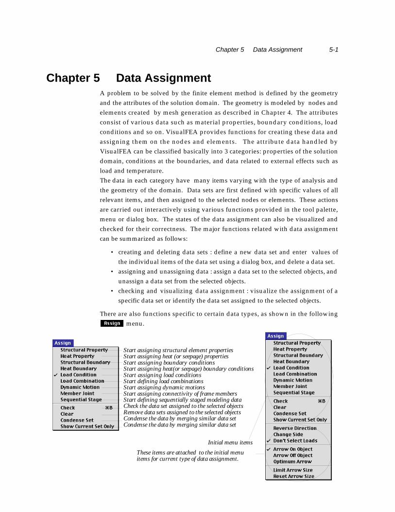
T h e re are also functions specific to certain data types, as shown in the following
menu.
Chapter 5 Data Assignment
These items are attached to the initial menu items for current type of data assignment.
Initial menu items
Start assigning structural element propertiesStart assigning heat (or seepage) propertiesStart assigning boundary conditionsStart assigning heat(or seepage) boundary conditionsStart assigning load conditionsStart defining load combinationsStart assigning dynamic motionsStart assigning connectivity of frame membersStart defining sequentially staged modeling dataCheck the data set assigned to the selected objectsRemove data sets assigned to the selected objectsCondense the data by merging similar data setCondense the data by merging similar data set

5-2 Chapter 5 Data Assignment
Overview of Data Assignment
There are a few different types of data to be assigned to the finite element model.
But the pro c e d u res of assigning data are similar and consistent re g a rdless of the
data type as described below.
Basic composition of data
The minimum amount of data necessary for finite element analysis is varied with
the type of problem to be solved. VisualFEA can do 3 types of analysis : structural,
heat conduction and seepage. And there f o re, data re q u i red for these 3 types of
problems are described below.
■ Data for structural analysis
The attribute data necessary for structural analysis are basically composed of the
following components:
• material properties: elastic constants, unit weight, thermal expansion
coefficients, etc.
• s t ructural boundary conditions: structural constraints or supporting states
such as spring.
• load conditions: various types of applied forces including uniform forc e ,
moment, body force, etc.
The above components are essential for structural analysis. Multiple load
conditions can also be defined by linear combination of the load condition sets.
• load combinations: combinations of load condition sets defining multiple
load condition. This item is available only for linear static structural model
with more than 2 load condition sets.
The following data items are additionally required to define other characteristics
of the problem.
• local member connectivity: pin ended, rigid ended.
• dynamic motion: dynamic displacement, velocity and acceleration.
When the necessary data are completely assigned, the problem are are ready for
finite element solution.
■ Data for analysis of heat conduction
The data necessary for heat conduction analysis are basically composed of the
following 2 components:
• material properties: thermal conductivities in X, Y and Z directions.

Chapter 5 Data Assignment 5-3
• heat and temperature boundary conditions: specified temperatur e s ,
specified heat flux, convection boundary conditions, heat source, etc.
In order to make the problem solvable by VisualFEA, the material pro p e r t i e s
should be assigned to all elements, and at least one component of the heat or
temperature boundary conditions should be applied.
■ Data for seepage analysis
The data necessary for seepage analysis are basically composed of the following 2
components:
• material properties: flow conductivities in X, Y and Z dir e c t i o n s ,
conductivity function, water content function.
• seepage boundary conditions: water head (open and confined), flux, point
source, and initial water table.
In order to make the problem solvable by VisualFEA, the material pro p e r t i e s
should be assigned to all elements, and an open or confined head boundary
condition should be applied at least to one point of the model, as subsequently
described
General procedure of data assignment
The pro c e d u re of assigning data, re g a rdless of type, may be divided into the
following several steps:
1) Start the data assignment procedure.
Choose one of the items “Element Property”, “Structural Boundary”, “Heat
Boundary”, “Load Condition”, and “Element Connectivity” fro m
menu. Then, a corresponding dialog box appears.
2) Define a data set.
A data set is a data unit carrying specific values of data items. There are a
number of items in a data set. Specific values are entered for them using the
associated dialog. Details of data items are described for each data type in the
following sections.
You may define as many data sets as necessary. There is no limit to the number of
data sets. Only one data set is active at a time. The currently active data set is
effective for assignment. When a new data set is created, the set becomes active
automatically.
3) Make the desired set active.
If you want to assign a data set which is not currently active, you should
make the desired set become the active one by scrolling. A data set may be
c reated, deleted or scrolled using the functions of dialog boxes, which are

5-4 Chapter 5 Data Assignment
explained later in this section.
4) Select objects to assign data.
A data set may be assigned to different types of objects, but not to all object
types. There is a default object type for a given data type. The selection tool
of default object type is automatically activated when you start a data
assignment procedure. You may switch the object selection tool if necessary,
but only applicable object selection tools are enabled.
5) Assign data to the selected objects.
Click button of the dialog to assign the currently active data set to the
selected objects. The newly assigned data are indicated with highlight on the
mesh.
Some types of data may be assigned to surface meshes, volume meshes or curves.
However, they are eventually assigned to the nodes or elements within these objects.
The default and applicable object types are described in detail for each data type in the
following sections.
You may repeat step 2) through 5) as many times as necessary without opening the
dialog again while the corresponding dialog box is on the main window. You may
quit this data assignment pro c e d u re by clicking the close box of the dialog, or
starting any other procedure.
Functions common to all types of data assignment
T h e re are a number of functions related to data assignment. Some of them are
p rovided as dialog items, and others as menu items. Among all the various
functions related to data assignment, those ones commonly applied to all types of
data assignment are described below. Other functions are applied diff e re n t l y
depending on the type of data and the analysis subject. So, they are explained in
separate sections for various types of data assignment.
■ Functions handling data sets
While you are assigning data, a dialog box is always displayed on the main
window. The dialog boxes have various items depending on the associated data
type and the analysis subject. However, there are items common to all dialog
boxes for data assignment as shown below.
create a new data set
delete a data set
scroll up data setsscroll down data sets
assign a data set
data set label
data set number
(Mac OS : popu menuWindows: dropdown list)

Chapter 5 Data Assignment 5-5
All of the above dialog items are for handling data sets including creating, deleting,
scrolling and selecting data set. Usage of the items is explained below.
Click this button to create a new data set. The values of the data items
in the new set are initially copied from the existing values if
applicable, or given with the default values.
The active data set is deleted by clicking this button. The data set is
also removed from all the objects assigned with it. Exceptionally in
case only one data set is left. Then the set is not deleted, but only its
assignment is removed.
The data set numbers are rearranged to fill the gap of the deleted set.
The set next to the deleted set becomes active.
Click this button to assign the current data set to the selected objects.
( Windows: It is the default push button of the dialog. There f o re ,
pressing key has the same effect as clicking this button.)
The number of the data set is displayed as a popup menu(Windows:
d rop-down list) item. You may choose the desired set using this
popup menu (Windows: drop-down list).
The label of the data set. You may label a data set by entering a
character string in the text box.
This button is used to scroll up the data set. The current set is scrolled
up by this button. Clicking this button once reduces the current set
number by one.
This button is used to scroll down the data set. The current set is
scrolled down by this button. Clicking this button once increases the
current set number by one.
■ Entering values of data items
A data set consists of many data items, each of which should be given with specific
values. All of the data items are expressed as dialog items: some are editable texts,
and others are radio buttons, check boxes, etc.
The first data set is initialized with the default values given by the program. When
a new data set is created, each item of the set usually inherits the value of the
corresponding item of the previously current set. Some items are interrelated.
You may freely enter or change values of the currently current data set before
assigning the set to objects. However, once a data set is assigned to any object,
modification of the set is restricted.
■ Modifying values of data items
In order to modify the values of a data set, first you must make the set the current
set using the dialog items , or as explained above. Only the current

5-6 Chapter 5 Data Assignment
set is displayed on the dialog, and thus, their items can be accessed for
modification. If the current set is not yet assigned to any object, the data items can
be edited freely. On the other hand, if the set is already assigned, modification of
the set either asks for confirmation or is not allowed. So, if you try to modify an
item of an assigned data set, you will get a message like this
If you click button, the current data become modifiable again so that you
may freely edit any item in the set until the modified set is assigned to any object.
In this case, the modification will affect all the objects assigned with this data set. If
you click button,the current set remains intact, and instead, a new set is
created. If you click button, your editing action is ignored, and nothing
happens.
There are also cases in which any assigned set cannot not be modified. Then, you
will get a notice like this,
If you click button, a new set is created and becomes current. So, you may
edit the data items of the new set and assign the set to the selected objects. If you
click button, your editing action is ignored, and nothing happens.
■ Assigning data sets
If new data assignment is ready, button of the dialog is enabled. Pressing
the button assigns the current data set to the selected objects. Data assignment can
be canceled by “Undo” command in menu before any other action is taken.
You may assign a data set to objects which have already been assigned with other
data sets. The results of such overlapping assignment depend on the type of data
and setting of the related option, and are explained in conjunction with assignment
of corresponding data sets.

■ Checking data assignment
The state of the data assignment can be checked using “Check” item.
When you choose “check” item in menu, the data set assigned on
the selected object becomes active, and the dialog shows the data items of
this set. At the same time, the assignment of the new current set is
displayed with highlight.
If two or more objects are selected and they are not assigned with a single
data set, the new current set cannot be determined, and thus re q u e s t e d
checking may not be realized.
Instead of using this function, you may identify the data set by scrolling
the current data set.
■ Clearing data assignment
In order to clear data assignment from certain objects, first select the objects to be
cleared of data assignment, and choose “Clear” item. All data sets of the current
dialog are unassigned from the selected objects. The data sets themselves are not
affected by this action.
In order to delete data sets, use button in the dialog.
■ Condensing data sets
If you want to remove data sets which are not assigned to any object, choose
“Condense” item. As for structural boundary conditions, data sets with identical
contents will also be merged into one by this action. If the current set is merged
into another set, the merged set becomes the current set.
■ Ending data assignment
In order to end the current data assignment, simply click the close box of the dialog
box, or start any other command.
Chapter 5 Data Assignment 5-7

5-8 Chapter 5 Data Assignment
Structural Element Properties
The attributes of the solution domain in finite element analysis are defined by the
data representing the characteristics of each element. These data are termed here
as element properties. The element property related action is initiated by one of
the 2 diff e rent menu items, i.e., "Structural Property" and "Heat Property" (or
"Seepage Property" for a seepage analysis) depending on the type of property for
assignment. In the case of coupled analysis, it is necessary to assign two different
types of properties to one model.
Defining structural element properties
In order to start assigning structural properties, choose “Structural Property”
item in menu. “Property” dialog appears, and the current state of
their assignment are displayed in the main window.
The element properties are defined and assigned by the data unit called
element property set. A set consists of many data items, all of which are
displayed on “Property” dialog. Structural element properties may include
geometric characteristics as well as material properties. The items diff e r
depending on the subject of analysis, or analysis class of the element as
described below.
■ Analysis class of element
The first popup menu in “Property” dialog is provided to enable mixing different
types of stru c t u res in one analysis, as explained in the next section. Using this
menu, you can select the type of analysis-related characteristics to impose on the
element. It is termed here as “analysis class of element.” Each item of the popup
menu represents an analysis class of an element.
check box to turn on or off property color mode
popup menu selecting the analysis class of the element
popup menu setting the constitutive model
buttons to set isotropy
editable text for data items consisting an element property set

Chapter 5 Data Assignment 5-9
• "Plane/Surface": plane stress, plane strain, axisymmetric, plate bending, and
shell element.
• "Solid": 3-d solid element.
• "Truss": 2-d or 3-d truss element.
• "Frame": 2-d or 3-d frame element.
• "Interface": interface or gap element
• "Slip Bar": slip bar element
• "Embedded bar": embedded bar element
• "Heat": heat conduction element
Only classes compatible for the current project are selectable. In case of frame
analysis, for example, "Truss" and "Frame" items are selectable, and others are
disabled.
■ Constitutive model
The second popup menu in “Property” dialog is to select the constitutive
model. This is applicable for material nonlinear analysis of stru c t u res. For
linear analysis, the menu contains only "Linear" item. The current version of
VisualFEA supports only those nonlinearities shown as the menu items. The
items vary depending on the analysis class of element as described in the
p revious section. For "Plane/Surface" and "Solid", the following items are
available.
• "Linear": linear elastic model.
• "Elasto-plastic:V-M": Elasto-plastic model with Von Mises yield criterion.
• "E l a s t o - p l a s t i c : M - C": E l a s t o - p l a s t i c model with M o h r- C o u l o m b y i e l d
criterion.
• "Elasto-plastic:Tresca": Elasto-plastic model with Tresca yield criterion.
• "E l a s t o - p l a s t i c : D - P": Elasto-plastic model with D ru c k e r- P r a g e r y i e l d
criterion.
• "Compression Only": Linear constitutive relationship for compression, and
no stress for tension.
• "Tension Only": Linear constitutive relationship for tension, and no stre s s
for compression.
The following are the items available for interface elements.
• "L i n e a r Interface": linear elastic properties defined in the longitudinal and
the thickness direction respectively.
• "No tension slip": The interface delivers compressive normal force across the
element, but not tensile force. The maximum resistance against slippage
between the two faces across the element is defined by the friction
c o e fficient. The maximum resisting stress is obtained by normal stre s s
multiplied by the friction coefficient.

5-10 Chapter 5 Data Assignment
• "No compression slip": The interface delivers tensile normal force across the
element, but not compressive force. The maximum resistance against
slippage between the two faces across the element is defined by friction
c o e fficient. The maximum resisting stress is obtained by normal stre s s
multiplied by the friction coefficient.
• "Gap": The interface models a gap between two faces. No force is delivered
between the two faces until the gap is diminished by deformation.
The following are the items available for slip bar elements.
• "Linear bonding": The bonding between the slip bar and the surro u n d i n g
body is represented by linear elastic model .
• "Nonlinear bonding": The bonding between the slip bar and the surrounding
body is represented by nonlinear stress-strain relationship.
■ Isotropy of the properties
The element properties can be defined as either isotropic or orthotropic using the
radio buttons in "P roperty" dialog. In case the properties are defined as
orthotropic, there appear more items in the dialog as shown in the following figure.
<Data items for isotropic materials and for orthotropic ones>
defined as isotropic
defined as orthotropic

Chapter 5 Data Assignment 5-11
■ Data items of element properties
An element property set consists of a number of data items, which vary depending
on the analysis subject, analysis class of the element and the isotropy. As you alter
the popup menu items or radio buttons on "Property" dialog, you will notice that
the dialog expands or shrinks in its size to accommodate the changing data items
p ro p e r l y. Each data item is denoted by a simple token or by a caption. This
denotation of data items can be toggled by clicking the part of the dialog as shown
in the figure below..
Defining element properties of truss and frame elements
Frame and truss elements are line segments with specific cross sections. The
property set of such elements includes the data related to the cross section such as
section area, area moment of inertia, and so on. These data can be defined either
directly inserting the values to the corresponding items, or indirectly by specifying
the shape and the dimensions of cross section.
" P roperty" dialog for frame or truss element is diff e rent from dialogs for other
analysis class elements as shown below.
There are 2 radio buttons to set whether to define the element properties with or
without defining the cross section. Turn on "Section unspecified" radio button to
define the element property without specifying the cross section. Otherwise, turn
on "Section specified" radio button to specify the cross section as explained in the
following section.
tokens of data items Click this part to toggletoken and caption
captions of data items

5-12 Chapter 5 Data Assignment
■ Defining cross sections of a truss or a frame member
The cross sectional properties of a structural member can be inputted by
dimensioning the section of a selected shape in the following order.
1) Click "Defined section" radio button or button.
Then, "Section Properties" dialog appears on the screen.
2) Scroll the list view of section icons so that the desired icon may be seen.
The current version of VisualFEA has 13 shapes of defined cross section. The
list view on the left of the dialog contains the icons of section shape. Only 4 of
Use these buttonsto set whether to specifythe cross section or not
Press these buttonsto create or modify a cross section
Click the icon to selectthe section type.
Dimensional notationsof the selected section typeare displayed here.
Set the orientationof the section.
Input dimensionsof the selected section type.
Set the scale of the inputted dimensions to actual ones.
Computed section porperties.
Click this button to insert the computed section properties into appropriate items of “Property” dialog.
Save the section attributes to a fileRead the section attributes from a file

Chapter 5 Data Assignment 5-13
<List view icons and dimensional notations of cross sections>

5-14 Chapter 5 Data Assignment
them are shown. The desired one can be made visible by using the scroll bar
of the list view.
3) Select the desired shape of cross section.
Click the icon of the desired shape. Then, there appears the detailed view of
the selected cross section with dimensional notations, and editable text boxes
for inputting the dimensions.
4) Input dimensions of the section.
Insert the texts into the editable text items representing the dimensions of the
c ross sections. If all the dimensions are supplied, the computed sectional
properties are displayed at the right bottom portion of the dialog.
5) Set the orientation of the section if necessary
If the desired orientation of the section is not the same as the one displayed on
the dialog, that can be altered by choosing one of the following radio buttons:
- "Original" : The orientation is maintained as it is.
- "Flip vertical": The section is flipped about a horizontal axis.
- "Flip horizontal": The section is flipped about a vertical axis.
- "Rotate right": The section is rotated 90° clockwise.
- "Rotate left": The section is rotated 90° counter clockwise.
- "Rotate 180° ": The section is rotated 180°.
6) Click button.
The computed cross sectional properties are automatically inserted into the
corresponding items of "Property"dialog.
< Automatic insertion of computed cross sectional properties>

Chapter 5 Data Assignment 5-15
Once the cross sectional properties are automatically inserted into the appropriate
text items of "Property" dialog, the cross section data is linked to the property set.
Thus, "Defined section" radio button is turned on for this set. The cross section of
this property set can be edited later by clicking button and modifying the
text items of "Section Properties" dialog. However, if any item automatically
inserted from the cross sectional definition is manually modified, the link between
the property set and the section properties is broken and cannot be re c o v e re d .
Thus, "Undefined section" radio button is turned on for this property set.
Assigning element properties
Element properties are assigned to objects as a set. Only the currently active set is
assigned to selected objects by clicking button of the dialog. The general
procedures of assigning data are explained in a previous section, and so will not be
repeated here. Rules of object selection for property assignment and the display of
the assignment are briefly explained below.
■ Selecting objects to assign element properties
Element property sets can be assigned to various objects. However, the data sets
a re eventually assigned to elements constituting the objects. For example,
assigning a data set to a volume is equivalent to assigning the set to all elements
within the volume. There f o re, the data sets can be assigned either to individual
elements or to the kind of objects which contain the actual elements involved in the
finite element analysis. The assignable objects differ depending on the analysis
subject or the analysis class of element as summarized in the following table.
< Assignable objects for element properties >
plane stress/strainaxisymmetric,plate bendingshell structure
3-D solid structure
2-D truss3-D truss
2-D rigid frame3-D rigid frame
interface
slip bar
embedded bar
plane/surface
volume
truss
frame
interface
slip bar
embedded bar
surface mesh, surface element
volume mesh, volume element
curve, truss element
curve, frame element
curve
curve
curve
analysis subject analysis class
of element assignable objects

5-16 Chapter 5 Data Assignment
■ Overriding previous assignment of element properties
If you assign a data set to objects on which another data set has already been
assigned, the newly assigned set will replace the old one. Thus, one data set at
most is assigned to an element.
Because of this overriding behavior, it is more efficient to start assigning property sets from
l a rger regions and to proceed to smaller parts. For example, if most of a mesh has one
property and a remaining small part has another, assign one property set to the mesh as a
whole first and another set to the relevant elements.
■ Representation of element property assignment
Elements assigned with element properties are drawn in red. The elements
assigned with the currently active data set are highlighted in dark red The
assignment is always represented by boundary lines of each element, regardless of
the rendering mode.
Mixing different structural types in one analysis
Different types of structures may be included in one analysis. For example, you
may model a 3-D solid stru c t u re in which 3-D truss members exist as shown
b e l o w. This can be achieved defining and assigning element property sets of
different analysis classes using the popup menu in “Property” dialog.
< Example of a model with mixed structural types >
■ Changing the analysis class of element
The popup menu in “Property” dialog has a few items re p resenting analysis
classes. When the dialog appears for the first time , the popup menu is set to the
item of analysis class corresponding to the current analysis subjects. If you change
the item, all the dialog items are also altered accord i n g l y. At the same time, the
assignable objects are changed, and the relevant object selection tool is
automatically activated.
3-D solid
3-D truss

Chapter 5 Data Assignment 5-17
■ Applicable analysis classes of element
In VisualFEA, not all types of structures can be mixed with each other. There are
applicable types for a given analysis subject. In the popup menu shown above,
only the items of applicable analysis classes are enabled. Listed in the following
table are the structural types which can be included for given analysis subjects.
< Structural types applicable for a given analysis subject >
plane stress/strainaxisymmetric
3-D solid structure
2-D rigid frame
3-D rigid frame
2-D truss2-D frameinterfaceslip barembedded bar
2-D truss2-D frameshellslip barembedded bar
2-D truss
3-D truss
trussframeinterfaceslip barembedded bar
trussframeplane/surfaceslip barembedded bar
truss
truss
analysis subject analysis class of element structural type
applicable structural types
Popup menu for selectingthe analysis class of element.

5-18 Chapter 5 Data Assignment
Using interface elements
Interface elements are used in modeling the behavior of gaps with negligible
width. They cannot be used alone, but may be included in plane stress, plane
strain or axisymmetric problems. (The current version of VisualFEA supports only
2 dimensional interface elements.)
■ Characteristics of interface elements
Interface elements fill the gap separating two adjacent surfaces. They connect the
nodes on the boundaries of both surfaces. VisualFEA supports only 4 node
interface elements. The structural behavior of the gap can be controlled by the
stiffness of the interface elements in width and length directions. These stiffness
are determined by the moduli of elasticity in both directions, and the gap width of
the elements. A pair of nodes facing with each other are separated by as much as
the specified gap width. Assigning zero or very small value of gap width or large
modulus of elasticity in width direction will restrain the relative movement in
width direction, of the pair of nodes. On the other hand, the modulus of elasticity
in length direction controls the relative movement in length direction. So, you may
model the desired behavior of the gap, or relative movement of the contacting
surfaces by assigning appropriate values to the properties of interface elements.
< Characteristics of interface elements >
■ Creating interface elements
Interface elements are created somewhat differently from other structural types of
elements. They are not created by mesh generation or curve input, but by
assignment of element properties as explained below.
1) Choose “Interface” item from the popup menu in “Property” dialog.
The data items in “Property” dialog are altered.
2) Enter the value for each data item.
The interface element can be made to represent specific behavior by entering
appropriate values for the data items.
surface 1
surface 2base curve Before generating interface elements After generating interface elements
interface elements
gap width
EL
Eg

Chapter 5 Data Assignment 5-19
• modulus of elasticity in length direction (EL): The Young’s modulus of
elasticity in the direction parallel to the length of the interface elements.
• modulus of elasticity in gap width direction (Eg): The Young’s modulus of
elasticity in the direction normal to the length of the interface elements.
• gap width (gap): The width of interface of elements. This value should be
small as compared with the dimension of the whole structure.
• thickness (t): This item is applicable only for plane stress problems. Usually,
this value is set as identical to the thickness of the main structure in which
the interface elements are embedded.
3) Select one or more base curves to assign interface elements.
The selected base curves are to be used as the basis of the interface elements.
T h e re f o re, they should be serially connected, and completely embedded
within the main structure.
4) Click button in the dialog.
Interface elements are created on the selected curves. The active set of
element properties are assigned to the newly created elements.
When interface elements are created, the basis curves together with the nodes on
them are duplicated. The interface elements are composed of the nodes on the new
and existing base curves.
< Example of a plane strain case with interface elements >
■ Deleting interface elements
Interface elements can be deleted only by deleting the set of element pro p e r t y
assigned to them. The meshes are re s t o red to the state before creating interface
elements. That is, the surface meshes separated by the interface elements are
joined again.
interface elements
plane strain elements
Before deformation After deformation

5-20 Chapter 5 Data Assignment
Using slip bars
Slip bar elements are used in modeling bars, cables, rods or other reinforcement in
planar or 3-D solid structures. For example, tendons within prestressed concrete
beams can be best modeled by using slip bars. Slip bars cannot be used alone, but
may be included in plane stress, plane strain, axisymmetric, or 3-D solid structures.
■ Characteristics of slip bar elements
Slip bars are objects embedded within, but independent from, a body of planar or
3-D solid. There can be bonding effects between the slip bar and the main body.
These behaviors are modeled by using slip bar elements, which are a kind of truss
elements combined with bonding effects. Conceptually, nodes on slip bar are
s u r rounded by the nodes paired within the main body. Numerically, a pair of
nodes, one in the slip bar and the other in the main body, are independent from
each other, but share identical coordinates.
A pair of nodes are allowed to slip against each other in the direction along the slip
bar element. But they are forced to move together in its normal direction. The
bonding effect between the slip bar and the main body is re p resented by the
stiffness against the slip of paired nodes.
< Concept of slip bar elements >
■ Creating slip bar elements
Slip bar elements are created somewhat differently from other structural types of
elements, but similar to interface elements. They are not created by mesh
generation or curve input, but by assignment of element properties as explained
below.
1) Choose “Slip Bar” item from the popup menu in “Property” dialog.
main body
slip bar
nodes on the main body
nodes on the slip barEach pair of nodes have identical coordniates

Chapter 5 Data Assignment 5-21
The data items in “Property” dialog are altered. A property set of slip bar
element is always accompanied by an annexed property set. The annexed set
has the attributes for truss elements re p resenting truss behavior of the slip
bar. This annexed set can be modified but cannot be assigned independently.
2) Enter the value for each data item.
The slip bar element can be made to represent specific behavior by entering
appropriate values for the data items.
• modulus of elasticity of the slip bar (Eb a r): The Young’s modulus of
elasticity of the slip bar elements.
• modulus of elasticity re p resenting ( Eb o n d): The Young’s modulus of
elasticity representing the bonding effect between the bar and the solid.
• section area (A): The section area of the bar.
3) Select one or more curves to assign slip bar elements.
The selected curves are to be used as the basis of the slip bar elements.
Therefore, they should be serially connected, and completely slip within the
main body.
4) Click button in the dialog.
Slip bar elements are created on the selected curves. The active set of element
properties are assigned to the newly created elements.
< Example of modeling a prestressed beam using slip bar elements >
■ Deleting slip bar elements
Slip bar elements can be deleted only by deleting the set of element pro p e r t y
assigned to them. When a property set for slip bar is deleted, its annexed set is
also removed.
Without prestressing With prestressing

5-22 Chapter 5 Data Assignment
Using embedded bars
Similarly to slip bars, embedded bars are also used in modeling stiffening material
embedded within planar or 3-D solid stru c t u res. Embedded bars are more
convenient and flexible to use than the slip bars, because they can be arbitrarily
placed within continuum. Embedded bars cannot be used alone, but may be
included in plane stress, plane strain, axisymmetric, or 3-D solid structures.
■ Characteristics of embedded bar elements
Embedded bars and slip bars are similar in their usage as stiffening line segments
embedded within continuum, but diff e rent in their characteristics and in their
modeling method. A slip bar is an element which has nodes and its own
displacement field, while an embedded bar is not an independent element but a
stiffening segment embedded within continuum elements. Thus, an embedded bar
has neither independent displacement field nor nodes. Its displacements are
defined only through the deformation of the surrounding elements. The stiffness
of the embedded bars are directly added to the surrounding elements. The strains
of embedded bars are computed from the displacements of the surro u n d i n g
elements.
An embedded bar can pass through a number of elements without restriction in
the position or in the direction of its path. Embedded bars may be placed freely
within continuum without involving nodal connectivity conditions as shown in the
f i g u res of this and the next pages. So, embedded bars can be employed
conveniently in modeling complex reinforcement within continuums, especially in
combination with unstructured meshes.
2-D Mesh
embedded bar
< An example of embedded bars placed within a 2-D unstructured mesh >

■ Creating embedded bars
Any straight line can be defined as an embedded bar by assignment of element
properties as explained below.
1) Create straight lines using the line tool .Many embedded bars with a certain regular arrangement may be cre a t e d
e fficiently by using duplication of curves. The figure at the bottom of this
page shows an example of thousands of embedded bars created mostly by
"Duplicate and Move" and "Duplicate and Revolve". Refer to "Duplicating
curves and surface primitives" section of Chapter 3.
2) Start property assignment procedure.Choose “Element Property” item from menu.
3) Choose “Embedded Bar” item from the popup menu in “Property” dialog.The data items in “Property” dialog are altered to the items of embedded
bars.
4) Enter the value for each data item.The data items are related to the axial stiffness of the embedded bar. It is
assumed that the section area of the embedded bar is subtracted from the
embedding elements. Let Ae and Ee be the section area and the elastic
Chapter 5 Data Assignment 5-23
The mesh of this part is hidden.
Thousands of rock bolts in tunnel linings are modeled by embedded bars.
< An example of embedded bars in a 3-D solid model >

5-24 Chapter 5 Data Assignment
modulus of the embedded bar, and Eo be the elastic modulus of the
embedding element. Then, the stiffness contribution of the embedding bar is
5) Select one or more lines to assign embedded bar properties.
6) Click button in the dialog.The selected curves turn into embedded bars only when the surro u n d i n g
continuum elements are assigned with element properties as illustrated by the
f i g u re below. The intersections of embedded bars and element edges are
marked by small circles.
< Creation of embedded bars>
■ Deleting embedded bar
The embedded bar properties are removed by deleting the embedded bar property
set, or by clearing the assigned property set. The line segments remain undeleted,
although the property assignment is removed.
The mesh of this part is assignedwith element properties.
The mesh of this part is not assignedwith element properties.
Before assignmentof embedded bar properties
All these lines are selected for assignment of embedded bar properties.
After assignmentof embedded bar properties
Embedded bars are created only in the part assigned with element properties.
k = Ae Ee − Eo( )

Color coding of property sets
P roperty sets can be coded by colors. If the property color mode is turned on,
assignment of property set to each part of the model is distinguished by the color
used for rendering the part either in wireframe or in shaded image. Any parts
without property assignment are re n d e red in gray. The default color codes are
predefined for the first 16 property sets. The color of each set can be altered using
the color palette functions of the corresponding operating system.
■ Turning on the property color mode
The property color mode is turned on by checking the "Prop. color" box of
"Property" dialog. The color box filled with the color of the current property set
and "Palette" button appear on the dialog when the property color mode is turned
on.
■ Changing or setting the property color
Click button to change the property color. Then, the color palette dialog
appears on the screen. The default color for the first 16 sets are shown in the
palette.(Windows only) You may change the default color, or set a new color code
for the property sets beyond the first 16 sets.
It should be noted that gray is the reserved color for rendering the part without
property assignment, and cannot be used as a property set color.
Check this box to turn onthe property color mode.
the color of the property set Click this button to change the color
Chapter 5 Data Assignment 5-25

5-26 Chapter 5 Data Assignment
Heat Conduction and Seepage Properties
The element properties for heat conduction or seepage analysis are defined and
assigned in the similar way as that of structural analysis. The related actions are
initiated by "Heat Property" (or "Seepage Property") item of menu.
Heat conduction properties
If the analysis subject is defined as a heat conduction problem, "Heat
Property" item appears in menu and is enabled. Choose the item in
o rder to start assigning heat conduction properties. “Property” dialog
appears, and the current state of their assignment are displayed in the main
window.
■ Defining heat conduction properties
Heat conduction properties include the thermal conductivity coefficients in X and
Y directions for 2-D heat conduction problems, and X, Y and Z directions for 3-D
heat conduction problems. If the conductivity is isotropic, click "Isotropic" button
in the dialog. Then, the dialog shows only one editable text item "K". If the
conductivity is orthotropic, click "Orthotropic" button. Then, the dialog shows the
editable text item of the thermal conductivity coefficient for each of the coordinate
axis directions. Inserting the value(s) in the editable text box(es) complete the
defining of heat conduction properties.
■ Assigning heat conduction properties
Heat conduction properties can be assigned only to surface meshes in the case of
plane and axisymmetric heat conduction problems, and only to volume meshes in
the case of 3-D heat conduction problems.
defined as isotropic defined as orthotropic
thermal conductivity coefficients
thermal conductivity coefficientin all directions

Seepage properties
If the analysis subject is defined as a seepage problem, "Seepage Property"
item appears in menu and is enabled. Choose the item in order to
start assigning seepage properties. “Property” dialog appears, and the
current state of their assignment are displayed in the main window.
■ Defining seepage properties
Seepage properties include the hydraulic conductivity coefficients in X and
Y directions for 2-D seepage problems, and in X, Y and Z directions for 3-D
seepage problems. The conductivity can be re p resented by one value for
i s o t ropic material as shown in the figure below. Check "Isotropic" radio
button to input the conductivity coefficients as isotropic material.
Seepage properties include conductivity functions for unconfined seepage analysis.
The conductivity function defines the ratio of the reduced conductivity to the full
conductivity as a function of pore pressure.
■ Defining hydraulic conductivity functions
A conductivity function is associated with each one of the seepage property sets.
Click button in the "Property" dialog to input a conductivity function for the
current property set. Then, "Hydraulic Conductivity Function" dialog appears on
the screen. The conductivity function can be defined either by equation or by table
using this dialog as described below.
1) Click button of "Property" dialog to open "Hydraulic Conductivity
Function" dialog.The dialog opens with default settings. The dialog consists of 2 parts as
Chapter 5 Data Assignment 5-27
defined as isotropic defined as orthotropic
thermal conductivity coefficients
thermal conductivity coefficientin all directions
to define the conductivity of soil with negative pore pressure
to define the water content function

5-28 Chapter 5 Data Assignment
shown in the figure below. The first part is used to define the hydraulic
conductivity function by an equation, and the other part to define the function
in tabular form.
2) Turn on "Define by equation" radio button to define the conductivity function
by an equation.The hydraulic conductivity factor c is computed as a function of negative pore
pressure P by the equation,
where a is the Gardner coefficient and n is a power factor.
The conductivity factor implies the ratio of the reduced conductivity in
negative pore pressure region to the full conductivity.
3) Insert the Gardener coefficient a, and power factor n.
The value of a is normally assumed between 0.001 and 0.1, and the value of n
between 2 and 4.
4) Turn on "Define by table" radio button to define the conductivity function in
tabular form.The hydraulic conductivity is defined by the tabulated relation between the
c =1
1 =a Pn
Turn on this botton to define conductivity by the equation.
Turn on this botton to define conductivity by the table.
to add or insert a new row in the table.
to delete the selected row in the table.
to read the table saved as a text file.
to save the table as a text file.
to display or edit the conductitity function in graphic mode.

p o re pre s s u re and the conductivity factor. The conductivity factor is
computed by linear interpolation of the given pore pre s s u res and the
conductivity factors.
5) Click button to add a new row in the table, and button
remove a row.
The buttons are enabled when "Defined by table" radio button is turned on.
After creating a new row, insert the values of the row using the editable text
box.
6) Click button to complete defining the conductivity function.
The "Hydraulic Conductivity Function" dialog closes, and the conductivity
function is added to the current seepage property set. The check box of
"Conductivity Func." item of the "Property" dialog is marked to indicate that
the hydraulic function of the property set is defined.
■ Assigning seepage properties
In order to assign seepage properties, first select the object to assign, and click
button of the "Property" dialog. Seepage properties can be assigned only to
surface meshes in the case of plane and axisymmetric seepage problems, and only
to volume meshes in the case of 3-D seepage problems.
Chapter 5 Data Assignment 5-29

5-30 Chapter 5 Data Assignment
Structural Boundary Conditions
S t ructural boundary conditions specify the way a stru c t u re is supported.
The data items of the structural boundary condition are related to the
constraining status of nodes at the boundaries. The status is defined for
each nodal d.o.f., and is one of the following four.
• free : free to move. In other words, no constraint is imposed.
• f ree with spring constant : partially constrained state like hinges with
friction, elastic supports, etc. The degrees of constraint are represented
by spring constants.
• fixed: No movement is allowed. The 0 displacement is prescribed.
• fixed with prescribed displacements : initial displacement, settlements,
etc. The displacement is forced to be the prescribed value.
In order to start assigning structural boundary conditions, choose “S t ru c t u r a l
Boundary” item in menu. “Struct Boundary” dialog appears, and current
state of their assignment are displayed in the main window.
Defining structural boundary conditions
You must first create and define sets of boundary conditions before assigning them
on the structural boundaries. All the data items of the active set are displayed on
”Struct Boundary” dialog and can be entered or modified using the dialog.
■ Nodal degrees of freedom
The boundary condition dictates the state of each nodal degree of freedom. The
nodal d.o.f. differ depending on the subject of analysis. If more than one structural
type is involved in the analysis, the items are extended to hold all associated
structural types.
fixity of each nodal d.o.f. prescribed displacements
or spring constants
content of editable text items
options of handling overlaid data sets
letters representing nodal d.o.f.
The boundary condition is defined in local coordinates
if this box is checked.

Chapter 5 Data Assignment 5-31
< Nodal d.o.f for various analysis subjects >
■ Data items of structural boundary condition
A structural boundary condition set has a few data items. They consist of nodal
fixity, initial displacements or spring constants defined for each d.o.f.
• f i x i t y: the state of nodal constraint. Either “free” or “fixed” condition is
specified for each nodal d.o.f., and indicated in the check boxes of the dialog.
If a box is checked, the corresponding d.o.f. is fixed.
• p rescribed displacement: nodal displacements given prior to solving the
problem. Nodal displacements can be specified only for fixed d.o.f.
• spring constant: This value represents the degree of partial constraint. The
spring constants can be specified only for free d.o.f.
The following figure shows examples of applying prescribed displacements and
spring constants.
< Nodal d.o.f for various analysis subjects >
■ Entering data items of boundary conditions
The fixity of each nodal d.o.f. is entered by clicking the check box in front of the
symbol indicating the respective d.o.f. The prescribed displacements and the
prescribed displacement

5-32 Chapter 5 Data Assignment
spring constants are entered within the corresponding text boxes. As shown
below, not all the text boxes are displayed. Some of them are hidden. Displayed
items are related to the heading of the text items. There are 3 headings:
• “ P rescribed Displace.”: This heading indicates that only text items for
p rescribed displacements are shown. Because displacements can be
prescribed only for fixed d.o.f., the text items of fixed d.o.f. are displayed.
• “Spring Constant”: This heading indicates that only text items for spring
constants are shown. Because spring constants can be applied only for free
d.o.f., the text items of free d.o.f. are displayed.
• “Mixed Values”: This heading indicates that text items for spring constants
as well as for prescribed displacement are shown. Thus, all text items are
displayed.
The heading is initially set as “Prescribed Displace.” You may scroll through the
above three headings by clicking any point over the heading. But, only applicable
ones will be scrolled. For example, if non-zero values are entered in pre s c r i b e d
displacements, “Spring Constant” will be skipped.
< Headings of editable text items >
These checked d.o.f. are fixed.
These unchecked d.o.f. are free.
indicates that the prescribed displacements are entered in the following text boxes.
Enter the prescribeddisplacements in these boxes.Leave 0 for no displacement.
Click here to scroll the heading.
indicates that the spring constants are entered in the following text boxes.
Enter the spring constants in these boxes.Leave 0 for no spring constant,i.e., for completely free d.o.f.
indicates that either prescribed displacements or spring constantsare entered depending on the fixityof the corresponding d.o.f.

Chapter 5 Data Assignment 5-33
■ Defining boundary conditions in local coordinates
The structural boundary conditions can be defined in either in global coordinates
or in local coordinates. The local coordinates are based on the axis of a structural
member, the tangent direction of a surface edge, or the normal to a surface. Check
"Local direction" box of "Struct Boundary" dialog in order to use local coordinates
for a boundary condition set. At the moment, the "Local direction" is checked, the
d.o.f. labels are altered as shown in the figure below.
< Boundary constraints in local coordinates >
Use of local coordinates may be most appropriate for roller support and spring
boundary condition which are illustrated in the figure below. The pre s c r i b e d
displacements and the spring constants are entered for the local coordinates in the
same way as for the global coordinates.
2-D trussplane stressplane strainaxisymmetric
3-D truss3-D solid 2-D frame
3-D frame shell plate
local coordiatesnot defined
translation in the axial direction
translation in the direction normal to axis (truss/ frame) or to surface (shell)
translation in the local x direction(shell)
translation in the local y direction
translation in the local z direction
axial rotation (shell)
rotation about the local y axis(shell)
rotation about the local z axis(shell)
spring constant
prescribeddisplacement
spring support defined in local coordinates
roller support defined in local coordinates
< Examples of boundary conditions defined in local coordinates >

5-34 Chapter 5 Data Assignment
In most cases, only the axial direction or the normal direction is concerned with the
boundary conditions in local coordinates. The axial and normal directions at every
node is determined in association with the object to which the boundary condition
is assigned.
• curve: In the case the boundary condition is assigned to a curve, the axial
(//) direction is defined as tangent to the curve at every node on the curve.
For planar models, the normal (⊥) direction is uniquely determined from the
axial direction. For 3-D models, the 2 normal (/y and /z) directions are
determined by vector operations of the unit axial vector, and the unit
vector in the global Z direction, .
w h e re and re p resent unit vectors in the local y and z d i re c t i o n s
respectively.
• surface mesh: In the case the boundary condition is assigned to a surface
mesh, the normal direction (⊥) is first determined at every node on the
surface mesh. And the 2 other (/x and /y) directions are determined byvector operations of the unit normal vector and the unit vector in theglobal Y direction, .
w h e re and re p resent unit vectors in the local x and y d i re c t i o n s
respectively.
• node: If the node belongs to only one curve or only one surface mesh, the
normal or the axial direction is determined by the curve and the surface.
But, if the node shared by multiple curves or by multiple surfaces, then the
program asks to choose the curve or the surface mesh to be used as the basis
for determining the local directions.
First, choose one of the two ratio buttons, "Set the tangent curve", or "Set the
tangent surface mesh. (For a frame or a planar problem, the second button is
dimmed, and the first button is turned on.) And select the curve or thesurface mesh for the basis of the local directions. Then, button
becomes active. Click the button to assign the boundary condition in local
coordinates.
This item is dimmed in the case of a frame,or a planar problem.
r v y
r v x
r v x =
r j ×
r n
r v y = r
n × r v x
r j
r n
r v z
r v y
r v y =
r k ×
r t
r v z =
r t ×
r v y
r k
r t

Chapter 5 Data Assignment 5-35
Assigning structural boundary conditions
The structural boundary conditions are assigned to objects as a set. The currently
active set is assigned to selected objects by clicking button of the dialog. It
is assumed that all the nodes are initially free. That is, none of the nodal d.o.f. are
constrained fully or partially at the beginning. Assigning a boundary condition set
is equivalent to modifying the unconstrained state of each nodal d.o.f. Thus, the
boundary condition sets are assigned only to the nodes, one or more d.o.f of
which are fixed or free with spring constant. It is meaningless to define or assign
a boundary condition set with all d.o.f. free. If you define such a set and assign it
to the selected objects, the assignment is ignored.
■ Selecting objects to assign structural boundary conditions
S t ructural boundary conditions may be assigned to nodes, curves and surface
meshes. However, the data sets are eventually assigned to nodes within the
objects. For example, assigning a boundary condition set to a surface mesh is
equivalent to assigning the set to all nodes within the surface mesh.
For a 3 dimensional solid, boundary conditions are usually assigned only to the
outer surfaces, or to nodes on these surfaces. Therefore, it is sometime necessary to
prevent assigning boundary conditions to nodes inside the volume inadvertently.
This can be done by checking “Shut Invisible Nodes” item in menu so that
the inside nodes become unselectable.
■ Replacing or adding previous assignment
When a new structural boundary condition set is assigned to a node with
previously assigned boundary conditions, the old set will be either replaced by or
added to the new one, depending on the mode of overlaying data sets.
In “Struct Boundary” dialog, there are two radio buttons, “Replace” and “Add”. If
“Replace” button is on, the old assignment is replaced by the new assignment. The
text data items are also replaced by the corresponding values of the new set.
If “Add” button is on, the resulting assignment is the union of the old and the new
assignments. The state of a d.o.f. is determined by bit ORing with ‘0’ for free d.o.f.
and ‘1’ for fixed d.o.f. If the editable text data of both old and new sets are of same
kind( both prescribed displacements or both spring constants), the item is filled
with the one whose absolute value is larger.
If there exists a boundary condition set identical to the one resulting from the bit
ORing, that set is assigned to the node with the overlaid boundary conditions.
Otherwise, a new set is created.

Mark the boundary condition by rectangleMark the boundary condition by numberMark the boundary condition by icon
Enlarge the size of the iconReduce the size of the icon
5-36 Chapter 5 Data Assignment
< Example of overlaying boundary conditions >
■ Representation of boundary condition assignment
Nodal assignment of structural boundary conditions is re p resented by icon,
number or rectangle marked at the node. Choose the desired option of marking
the boundary conditions from menu. The item of the currently applied
option is checked as shown below. The icon option is available only for 2-D
modeling.
Boundary condition set 1 is applied to this curve first.
with “ Replace” button on with “ Add” button on.
The boundary condition set 3 is applied to this curve next
Set 1 is replaced by set 2. Set 3 is created and assigned
Boundary condition set 1 and set 2 are overlaid on this node.
1
2
3

Chapter 5 Data Assignment 5-37
<Options of representing boundary conditions>
If a boundary condition set is assigned to curves or surfaces, the individual nodes
on the curves or surfaces are marked. The nodes assigned with the currently active
data set are highlighted in dark red, and the nodes with other sets are marked in
bright red. The boundary conditions are displayed only when“Struct Boundary”
dialog is on the screen. Check "Show Str. Boundary" item of menu to make
the boundary conditions displayed even when “Struct Boundary” dialog is not on.
The size of the icon re p resenting the boundary conditions can be enlarged or
reduced by using "Enlarge" or "Reduce" item of menu.
Mark by rectangle
Mark by number
Mark by icon
fixed end roller support pin support

5-38 Chapter 5 Data Assignment
Heat Conduction and Seepage Boundary conditions
A menu item of menu is displayed in one of the two texts"Heat
Boundary" and "Seepage Boundary", depending on whether the analysis subject of
the project is heat conduction analysis or seepage analysis.
The boundary conditions in heat conduction and seepage analysis can be defined
and assigned by choosing the menu item.
Heat conduction boundary conditions are relevant only for heat conduction
analysis. Accordingly, “Heat Boundary” item in the menu is enabled only when
the analysis subject is set as one of the "Heat Analysis" item in”Problem Setup”
dialog. Likewise, seepage boundary conditions are relevant only for seepage
analysis. The text of the menu item displayed as "Seepage Boundary" when the
analysis subject is set as one of the "Seepage Analysis" item.
Defining heat conduction boundary conditions
You must first create and define sets of heat conduction boundary conditions
before assigning them on the heat conduction model.
■ Types of heat conduction boundary condition
There are a few different types of heat conduction boundary conditions as follows:
• temperature: A temperature is specified for various objects such as nodes,
curves and surfaces.
• c o n v e c t i o n: The convection coefficient and the ambient temperature are
assigned to an edge curve or a boundary surface .
• heat flux: The heat flux through a curve or a face is specified.
• point sourc e: A node is defined as a heat source. Heat source is more
analogous to load condition of structural analysis, and may be treated as
such. In VisualFEA, however, heat source is treated as a kind of boundary
condition.
editable text items
data type popup menu
specified temperatureconvection boundary conditionspecified heat fluxheat source or sink at a point
Chapter 5 Data Assignment 5-39
The type of heat conduction boundary condition is chosen using the popup menu
in “Heat Boundary” dialog. The editable text items are altered subsequent to
selection of the popup menu.
■ Editable text items
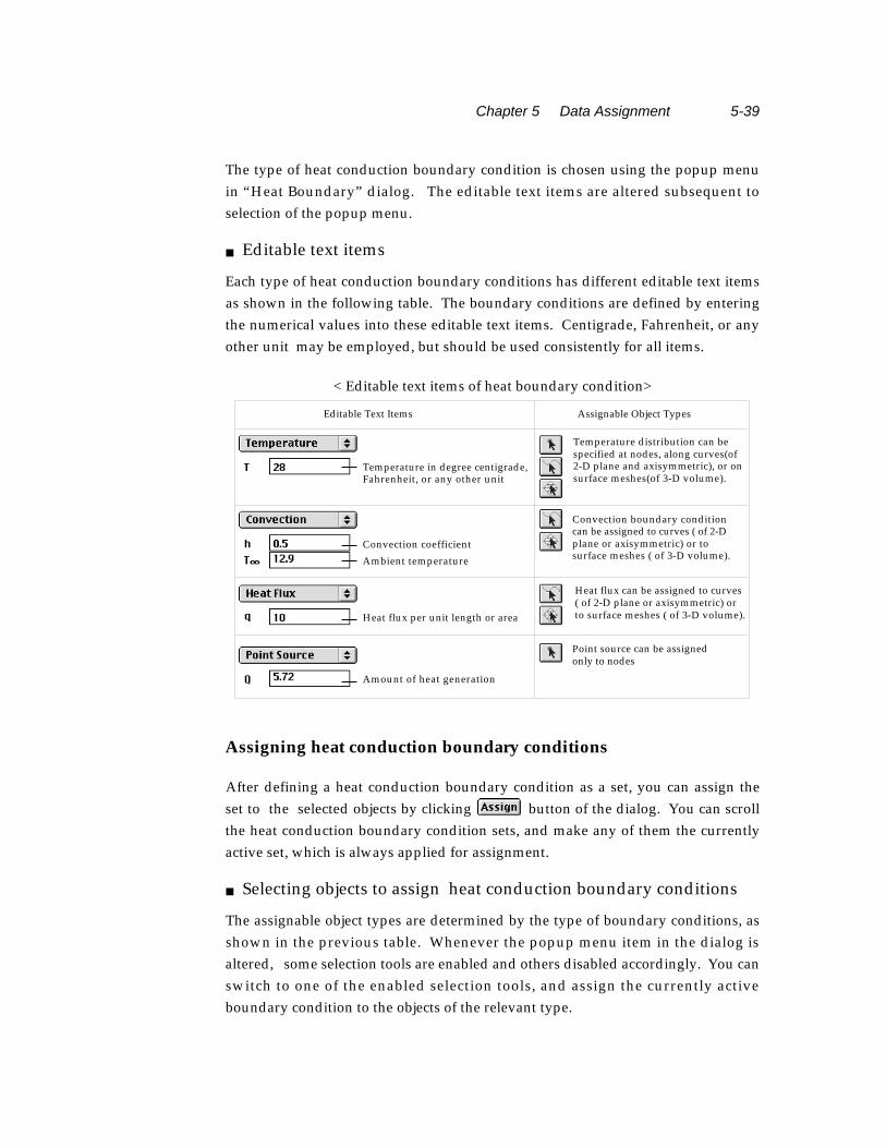
Each type of heat conduction boundary conditions has different editable text items
as shown in the following table. The boundary conditions are defined by entering
the numerical values into these editable text items. Centigrade, Fahrenheit, or any
other unit may be employed, but should be used consistently for all items.
< Editable text items of heat boundary condition>
Assigning heat conduction boundary conditions
After defining a heat conduction boundary condition as a set, you can assign the
set to the selected objects by clicking button of the dialog. You can scroll
the heat conduction boundary condition sets, and make any of them the currently
active set, which is always applied for assignment.
■ Selecting objects to assign heat conduction boundary conditions
The assignable object types are determined by the type of boundary conditions, as
shown in the previous table. Whenever the popup menu item in the dialog is
altered, some selection tools are enabled and others disabled accordingly. You can
switch to one of the enabled selection tools, and assign the currently active
boundary condition to the objects of the relevant type.
Editable Text Items Assignable Object Types
Temperature distribution can be specified at nodes, along curves(of 2-D plane and axisymmetric), or on surface meshes(of 3-D volume).
Convection boundary conditioncan be assigned to curves ( of 2-Dplane or axisymmetric) or tosurface meshes ( of 3-D volume).
Heat flux can be assigned to curves( of 2-D plane or axisymmetric) orto surface meshes ( of 3-D volume).
Point source can be assignedonly to nodes
Temperature in degree centigrade, Fahrenheit, or any other unit
Convection coefficient
Ambient temperature
Heat flux per unit length or area
Amount of heat generation

5-40 Chapter 5 Data Assignment
■ Replacing previous assignment
An object can be assigned with only one heat boundary condition set. If you assign
a new set to the object which has already been assigned with other set, the old set
will be replaced by the new one.
But, it should be noted that one object may encompasses other objects of different
type, and accordingly multiple sets may actually be assigned to a single object. For
example, a temperature may be specified along a curve, while the other
temperature is assigned to a node which is on the same curve. Thus, the node is
assigned with two condition sets which are in conflict. In this case, the nodal
assignment overrides other assignments such that the temperature of the curve is
not applied to that node. In general, if one object encompasses the other object,
and both objects are assigned with two different heat boundary condition sets, the
assignment on the encompassed object always overrides the other assignment.
■ Representation of heat conduction boundary condition assignment
The objects assigned with heat conduction boundary conditions are distinguished
f rom others by small square marks or by color. The nodes assigned with the
current set are marked by dark red squares. The nodes assigned with other than
the current set are marked by bright red squares. The curves, surface meshes, or
volume meshes assigned with the current set are drawn in dark red color, and
those assigned with other than the current set are drawn in bright red color.

Chapter 5 Data Assignment 5-41
Seepage boundary conditions
If the analysis subject is set as either "2-D Seepage", "Axisymmetric Seepage", or "3-
D Seepage", the text of the menu item "Heat Boundary" changes to "Seepage
Boundary". Selection of the menu item pops up the "Seepage Boundary" dialog.
Seepage boundary conditions can be defined and assigned, while the dialog is on
the screen,
■ Types of seepage boundary condition
T h e re are a few diff e rent types of seepage boundary conditions as described
below:
• open head: Open head is a type of boundary condition assigned to the
domain boundary curves or surfaces such as a upstream or a downstre a m
face of a dam. The boundaries assigned with open head include nodes
under and above the specified water head. The nodes under the specified
head are prescribed with the water head in the system equations. The nodes
above the specified head are so called "review nodes" subject to unknown
phreatic water face which are determined through iterative solution process.
The open head allocated review nodes automatically to the nodes above water level.
• confined head: Confined head is a type of boundary condition pre s c r i b i n g
all the assigned nodes with the specified water head .
• flux: seepage flow rate through unit area or length.
• point source: flow supplied at a point.
• initial water table: water table at the initial stage of transient seepage flow,
or water table initially assumed in the iterative solution process.
■ Assigning open head boundary conditionOpen head boundary conditions can be assigned using "Seepage Boundary" dialog by the
following pro c e d u re s .
1) Set the popup menu (Windows: dropdown list) to "Open Head".
data type popup menu
editable text items
free surface head (variable)confined head (fixed)seepage fluxseepage source or sink at a pointinitial water table

5-42 Chapter 5 Data Assignment
2) Insert the value of the water head in the editable text box with label "H".The upstream water level H1 and the downstream water level H2 a re the
values of the open water heads in the example below.
The water levels are measured from the datum to be specified in "Analysis Option"
dialog. Refer to "Setting analysis options for seepage analysis" section of Chapter 6.
3) Select the boundary curves or surfaces to be assigned with the open head..Select curves for 2-D analysis and surfaces for 3-D analysis.
4) Assign the boundary condition to the selected objects by clicking
button of the dialog.
<Example of open head boundary conditions>
■ Assigning confined head boundary condition
As an alternative to the open head boundary condition in the above example, the nodes of
the upstream edge under the water level can be assigned with "Confined Head" H1, because
the nodes of the upstream edge cannot form a phreatic water face above the upstream
water level. However, it should be noted that the confined head should assigned
only to the nodes under the upstream water level.
<Example of a confined head boundary condition in unconfined seepage analysis>
Assign “Confined Head” H1 to these nodes.
Assign “Open Head” H2 to this curve
Assign “Open Head” H1
to this curveAssign “Open Head” H2 to this curve
Specify this value in “Seepage Analysis Option” dialogH0 =Datum
H1
H2

Chapter 5 Data Assignment 5-43
The above example is to show that a confined boundary condition may substitute an open
head boundary condition in some cases. But confined boundary conditions are commonly
used to prescribes the constant head at the selected nodes or nodes along the selected curve,
as shown in the example below. In the case of confined seepage analysis, only confined head
conditions are applied.
In order to assign confined head boundary conditions, set the popup menu(Wi n d o w s :
d ropdown list) to "Confined Head," and follow the similar pro c e d u re as that of open head
boundary condition.
<Example of confined head conditions in confined seepage analysis>
■ Assigning flux
Water supply or drain through the boundary surfaces is re p resented by the boundary
condition of flux. In order to assign fluxes, set the popup menu(Windows: dropdown list) to
"Flux". The value of the flux should re p resent volume of water per unit area per unit time.
The flux should be assigned to boundary curves in 2-D seepage analysis and to boundary
surfaces in 3-D seepage analysis.
■ Assigning point source
Water supply or drain at a point is re p resented by the boundary condition of point source. In
o rder to assign point sources, set the popup menu(Windows: dropdown list) to "Point
S o u rce". The value of the point source should re p resent volume of water per unit time. The
point source should be assigned to nodes.
H1
H2
Assign “Open Head” H1
to this curveAssign “Open Head” H2
to this curve

5-44 Chapter 5 Data Assignment
■ Defining the initial water table
In transient analysis, the initial water table should be defined as the phreatic surface at the
initial stage. But in steady state analysis, the initial water table can be considered as the
initially assumed phreatic water surface, and there f o re, defining the initial water table may
not be essential. However, the assumption of the initial water table affects the computational
e fficiency of the iterative solution process, and is essentially used in obtaining the overall
distribution of the negative pore water pre s s u re above phreatic surface. The negative pore
water pre s s u re above the initial water table is set to 0.
The initial water table can be defined by the following pro c e d u re .1) Create a curve or a surface to be defined as the initial water table.
The initial water table is defined by one or more curves in 2-D seepage
analysis, and one or more surface meshes in 3-D seepage analysis. The curves
or surface meshes can be created as usual. If there already exist curves or
surface meshes that can be defined as the initial water table, this step can be
ignored.
2) Open "Seepage Boundary" dialog if it is not yet opened.
3) Set the popup menu (Windows: dropdown list) to "Initial Water Table".
4) Select the curves or the surface meshes to be defined as the initial water
table.
5) Click button of the dialog.
<Example of initial water table>
initial water table

Chapter 5 Data Assignment 5-45
Load Conditions
The load condition re p resents the state of various forces applied to the
objects in structural analysis.
In order to start assigning load conditions, choose “Load Condition” item in
menu. “Load Condition” dialog appears, and the current state of
their assignment is displayed in the main window.
Defining load condition sets
Load conditions are defined and assigned by the data unit called a load condition
set. A load condition set is initially created by clicking button of “Load
Condition” dialog. If a load set is already assigned, additional assignment of the
set, either to a single object or multiple objects, creates a new load set
automatically by duplicating the set. Loads applied to the assigned object(s) share
the new load set.
■ Data items of a load condition
A set consists of many data items including the type, the direction, the magnitude,
and the position of a force. The actual data items vary depending on the type of
analysis.
• load type: A number of load types are included in the first popup menu of
“Load” dialog.
• load direction: The local directions such as normal and tangential, as well as
x, y and z directions in the global coordinates are provided in the second
popup menu of the dialog.
• editable text items: Magnitude, position, re f e rence points and others are
inputted in the editable text items in the dialog. The editable text items
differ depending on the type of the objects.
■ Load types
load direction popup menu
load type popup menu
editable text items
load drawing scale

5-46 Chapter 5 Data Assignment
There are a number of different load types as shown in the the popup menu items.
Some of the menu items are enabled, while others are disabled depending on the
type of analysis. For example, “Point Force” item is available only for 2-D or 3-D
frames.
• nodal force: Nodal forces are applied at nodes. When this item is chosen in
the popup menu, the node selection tool is automatically activated, so
that you may select nodes to which the force is applied.
• point forc e: Point forces are applied at a point between nodes on a frame
member. This item is enabled only for 2-D and 3-D frame analysis. When
this item is chosen in the popup menu, the element selection tool i s
automatically activated.
• uniformly distributed: These are forces distributed uniformly over a curve or
a surface. In order to apply uniform forces, you must first activate the curve
selection tool , or the surface selection tool , unless one of the two
tools is already in action.
• linearly distributed: These are distributed forces with linear variation along
a curve. When this item is chosen in the popup menu, the curve selection
tool is automatically activated.
• parabolically distributed: These are distributed forces with quadratic
variation along a curve. When this item is chosen in the popup menu, the
curve selection tool is automatically activated.
• bilinearly distributed: These distributed forces have bilinear variation on a
surface. The force intensity at a point is determined by bilinear interpolation
of the intensities at 4 corner points. When this item is chosen in the popup
menu, the curve selection tool is automatically activated.
• nodal moment: This re p resents a moment or a couple applied at a node.
When this item is chosen in the popup menu, the node selection tool is
automatically activated.
Body forceSelf-straining forceThermal load
Concentrated force at a nodal pointPoint force at a point of a frame memberUniformly distributed forceDistributed force with linear varialion along a lineDistributed force with quadratic variation along a lineDistributed force with bilinear variation on a surfaceMoment at a nodal pointMoment at a point of a frame memberUniformly distributed momemt along an edge
Distributed force with hydrostatic variation in x dir.Distributed force with hydrostatic variation in y dir.Distributed force with hydrostatic variation in z dir.

Chapter 5 Data Assignment 5-47
< Examples of load types >
• point moment: This re p resents a moment or a couple applied at a point
between nodes on a frame member. This item is enabled only for 2-D and 3-
D frame analysis. When this item is chosen in the popup menu, the element
selection tool is automatically activated.
• uniform moment: This re p resents a line moment applied uniformly on a
frame member or an edge of a surface.
• body forc e: This is the force due to acceleration of mass. One example of
body force is the weight, or gravitational force of an object. Body force is
applicable to all types of objects except slip bar and embedded bar elements.
• self-straining force: This is internally exerted force due to prestressing, lack
of fit, and so on. Self-straining force can be applied to frame members or
embedded bar elements.
• thermal load: Thermal load implies the temperature variation or
t e m p e r a t u re gradient which causes strains and stresses. The equivalent
NodalForce
UniformForce
TrapeziformForce
ParabolicForce
PointForce
NodalMoment
PointMoment
UniformMoment
LoadType
LoadType
2-D Frame and 2-D Elasticity Example 2-D Frame Example

5-48 Chapter 5 Data Assignment
nodal forces are computed from the give temperature distribution. In a
coupled analysis of str u c t u re and heat conduction, the temperature
distribution is not specified by the thermal load but is given by the nodal
values computed from heat conduction analysis.
• h y d rostatic in X: “Hydrostatic in X” implies linear variation in the X
d i rection. This is to re p resent forces distributed on an area with intensity
varying linearly in X direction and uniform in other directions.
• h y d rostatic in Y: “Hydrostatic in Y” implies linear variation in the Y
d i rection. This is to re p resent forces distributed on an area with intensity
varying linearly in Y direction and uniform in other directions.
• h y d rostatic in Z: “Hydrostatic in Z” implies linear variation in the Z
direction. This is to represent forces distributed on an area with intensity
varying linearly in Z direction and uniform in other directions.
■ Load direction
The direction of forces may be specified either in X, Y, and Z axis of Cartesian
coordinates system or in local directions normal or tangential to curves or surfaces.
• X direction: X direction in XYZ coordinate system.
• Y direction: Y direction in XYZ coordinate system.
• Z direction: Z direction in XYZ coordinate system.
• normal to curve: Direction normal to the curve on which the force is acting.
• tangent to curve: Direction tangential to the curve on which the force is
acting.
x direction in Cartesian coordinatesy direction in Cartesian coordinatesz direction in Cartesian coordinatesDirection normal to a curveDirection tangential to a curveDirection normal to a surfaceDirection tangential to a surface and orthogonal to x axisDirection tangential to a surface and orthogonal to y axisDirection tangential to a surface and orthogonal to z axis

Chapter 5 Data Assignment 5-49
< Direction of a uniform load applied to a curve >
• normal to surface: Direction normal to the surface on which the force is
acting.
• tangent to surface and normal to X: The direction tangential to the surface
on which the force is acting, and normal to X direction. The dire c t i o n
tangential to a surface is not unique. The direction is constrained to be
normal to X direction, so that it became unique.
• tangent to surface and normal to Y: The direction tangential to the surface
on which the force is acting, and normal to Y direction.
• tangent to surface and normal to Z: The direction tangential to the surface
on which the force is acting, and normal to Y direction.
• no direction: This item is provided only for a thermal load which does not
have a direction. The load direction popup item automatically turns to this
item when the current load type is set as thermal load.
Tangent to CurveX Direction Normal to Curve

5-50 Chapter 5 Data Assignment
< Directions tangent to surface >
■ Editable text items
The editable text items are different depending on the type of loads as shown in the
following figures. When the popup menu item of load type is selected,
c o r responding editable text items appear on the dialog. The numerical values
related to a force are specified by these editable text items.
< Editable text items of load conditions >
X
Y
Z
Y
Z
X
Y
Z
X
Y
Z
X
X
Y
Z
X
Y
Z
Tangent to surfaceandnormal to X axis
Tangent to surfaceandnormal to Y axis
Tangent to surfaceandnormal to Z axis

Chapter 5 Data Assignment 5-51
< Editable text items of load conditions (continued)>
force magnitude
force intensity per unit length orper unit area
force magnitude
force location by ratio
force intensity at the other end
force intensity at one end
force intensity at mid point
force intensity at one end
force intensity at the other end
Editable Text Items Assignable Object Types
Nodal forces can be assigned only to nodal points. If “Nodal Force” is chosen as the type of load to assign, the node selection tool is automatically activated.
Point forces can be assigned only to a frame member. Therefore, this load type option is enabled only for 2-D or 3-D frames. Point forces can be applied either to elements (frame member) or to curves.The force location can be specified either by ratio(d/L) or by distance(d).
force location by distance
Click here to toggle d/L and d.
Uniformly distributed forces can be assigned to elements (except solid elements), to curves or to surface meshes.This type of force cannot be applied to solid elements.
Linearly varying trapesiform forces can be applied only to curves.In order to assign linear varing forces to surface meshes, use “Hydrostatic in X”, “Hydrostatic in Y” or “Hydrostatic in Z”
Quadratically varying parabolic forces can be applied only to curvesor frame elements.
1.0
force location by ratio force location by distance
Bilinearly varying distributed forces can be applied only to surface meshes.
w1 at corner 1
w2 at corner 2
w3 at corner 3
w4 at corner 4
w4
w1
w2
w3
d/LP P
d
L
w1
w2
w3
w1
w2

5-52 Chapter 5 Data Assignment
< Editable text items of load conditions (continued)>
Nodal moment can be applied to nodes of frame members. Therefore,this popup menu item is enabled only for frame analysis.
magnitude of moment
moment location by ratio
Editable Text Items Assignable Object Types
Point moments can be assigned only to a frame member. Therefore, this load type option is enabled only for 2-D or 3-D frames. Point moments can be applied either to elements (frame member) or to curves. The moment location can be specified either by ratio(d/L) or by distance(d).
force location by distance
magnitude of moment
Click here to toggle d/L and d.
Uniformly distributed moments can be applied to frame elements or to edges of a shell or a plate. Therefore, this type of load is valid only for 2-D frame, 3-D frame, plate bending and shell models.
Body forces can be assigned to elements, curves(for frames only), surface meshes(for planar elasticity, plate and shell), and volume meshes(for 3-D solid)
1.0
moment location by distance
moment location by ratio
moment intensity per unit length
Fb=wo abody force
unit massacceleration
acceleration
The magnitude of body force is determined by the acceleration and the unit mass which is specified as an item of the element property
average temperature
temperature gradient
thickness
Thermal loads can be applied to frame elements and curves. This type of load is valid only for 2-D and 3-D frame.
M
d/L
M
dL
M
M
T1
T2
Tav
Tgr
Tgr = T2 − T1
t
t

Chapter 5 Data Assignment 5-53
Self-straining forces can be applied to elements and curves, which should be members of truss or frame structures, or embedded bars within solids.magnitude of straining force
“Hydrostatic in X”
Object of assignment
Editable Text Items Assignable Object Types
force intensity w at X=h1
force intensity w at X=h2
force intensity w at Y=h1
force intensity w at Y=h2
force intensity w at Z=h1
force intensity w at Z=h2
X coordinate at which w=P1
X coordinate at which w=P2
Y coordinate at which w=P1
Y coordinate at which w=P2
Z coordinate at which w=P1
Z coordinate at which w=P2
“Hydrostatic in X”,“Hydrostatic in Y”, and “Hydrostatic in Z” can be applied to elements (surface elements only), curves and surface meshes.
P2
P1
h1
h2
X
X=0

5-54 Chapter 5 Data Assignment
Defining load condition sets for dynamic analysis
For dynamic analysis, load conditions may or may not have time dependent
characteristics. Therefore, assignment of dynamic load conditions involves more
steps than that of static load conditions, as described below.
■ Setting the time dependency
The dynamic load condition is classified further its time dependency as follows.
• static: static load condition independent of time.
• harmonic: time-dependent load condition with periodically changing
magnitude expressed by a sinusoidal equation.
• transient: time-dependent load condition represented in multiple time steps.
Thus, “Load Condition” dialog for dynamic analysis has radio buttons, "Static",
"Harmonic" and "Transient." Time dependency of a dynamic load is set by turning
on the corresponding radio button on "Load Condition" dialog.
As you alter the time dependency, you will notice the changing items below the
radio buttons. Time dependent attributes of dynamic loads are defined and
modified using these items.
■ Defining static load for dynamic analysis
Static load condition is assumed to have constant magnitude, direction and
position throughout the whole duration of analysis, and can be defined and
assigned in the same way as for static analysis. "Static" radio button should be
turned on to start defining static loads.
■ Defining harmonic load for dynamic analysis
A harmonic load has periodic characteristics with changing magnitude expressedby the sinusoidal function . The intensity of the load acting at asin t − to( )
radio buttons to setdynamic load classification
additional items fordynamic loads

Chapter 5 Data Assignment 5-55
specific time is obtained by multiplying the function by the constant load intensity
given at the bottom of the dialog.
■ Defining transient load for dynamic analysis
A transient load is defined by a series of values at a number of time steps, which
can be created and edited by the following steps.
1) Turn on “Transient” radio button in “Load Condition” dialog.
Then, items below the radio buttons take on the appearance shown below.
They include the current step number and the current time. The current time
step can be edited by directly changing the number in the box, or by scrolling
the number.
2) Click button.
Then, "Load Time Series" dialog pops up. The dialog produces editable
data items for each time step you create. The data items are equivalent to the data
items in "Load Condition" dialog.
current time step
current time
force magnitude
Click this button to create and edit a transient load
position of load
starting timeof application
ending timeof application
sin t − to( ) constant load intensity

5-56 Chapter 5 Data Assignment
3) Click button to add a time step.
A line of data items will be created for the new time step. In order to delete a
time step, click button after selecting the corresponding data line.
4) Select a line or a cell to edit.
Then, the data on the line or in the cell will be reflected in the editable text
boxes at the bottom of the dialog
5) Edit the text in the editable text box.
As you edit the text in a text box, it will immediately be echoed in the actual
data line.
6) Click button after completing creation of time steps.
"Load Time Series" closes and the data from the dialog are automatically
reflected in "Load Condition" dialog.
The data on the last line are assumed to be maintained up to the last time step in
the analysis. Thus the data shown in the above example dialog will create the
following time series data.
< An example of transient load>
0 0.2 0.4 0.6 0.8 1.0 1.2
0
-2
2
4
6
time
P

Chapter 5 Data Assignment 5-57
Assigning load condition sets
A load condition set is defined as explained in the previous section. The next step
is to assign the set to a certain object. You can assign the currently active set to
selected objects by clicking button of the dialog.
■ Selecting objects to assign load conditions
The load condition sets may be applied to various objects. However, assignable
object types are limited and determined by the type of load conditions, as
indicated in the previous figures of “Editable text items”. Only the selection tools
of assignable objects are enabled and others are disabled, whenever the type of the
current load set is altered.
■ Assigning a load condition set to multiple objects
You can apply the current load condition set to more than one object. However,
once the set is assigned, extra new load condition sets are automatically generated
so that each of the selected objects is assigned with an independent set which has
the same characteristics as that of the current set. So, you will find that the
number of load condition sets is increased as much as the number of assigned
objects minus one.
■ Assigning multiple load condition sets to a single object
One object may be assigned with more than one load condition sets. But there is a
possibility that you assign, by mistake, an identical load conditions to the same
object more than once. In order to prevent such a trouble, VisualFEA does not
allow assigning the same load condition to one object twice or more.
■ Representation of load assignment
The assigned forces, except body forces, are represented by arrows indicating the
point and the direction of their application. Body forces are indicated by x mark,
instead of arrow, at the centroid of each element.
The size of arrow can be adjusted using the slide bar of load drawing scale. The
slide bar has relative scale of arrow size. The arrow size can be lengthened by
moving the thumb of the bar to the right, and shortened by moving the thumb to
the left.
< Load drawing scale >
Enlarge the arrowReduce the arrow
Relative arrow size

5-58 Chapter 5 Data Assignment
Other functions related to assigning load conditions
Load conditions can be defined and assigned while the load condition dialog
appears on the screen. At this time, the few menu items related with load
conditions are attached to menu as shown below.
■ Reversing the force direction
The direction of the force can be reversed by simply choosing the item “Reverse
Direction” from menu. The force direction of the current load condition
set is reversed, and accord i n g l y, the corresponding editable text items of “Load
Condition” dialog is altered with reversed sign. If a load condition set is applied to
multiple objects, and “Reverse Direction” command is issued immediately, then
the direction of all the lastly assigned loads will be reversed.
< Result of “Reverse Direction” command>
■ Exchanging the reference end of the curve
The location of point force is represented by the distance from one end of a curve
or a frame element. In this case, the starting point of distance is the reference end of
the curve or the element. The magnitude of trapezoidal force is represented by two
load intensity W1 and W2. The end point with W1 may be the reference point . It
is sometimes necessary to switch the re f e rence point. This can be done simply
choosing the menu item “Change Side” from menu.
Reverse the direction of forceChange the reference end side of the curveSuppress selection of load by mouse clickDisplay the force simbol with arrow toward the object Display the force simbol with arrow outward the objectDisplay the force simbol with optimaly placed arrowLimit or do not limit the size of the force simbolReset the size of the force simbol
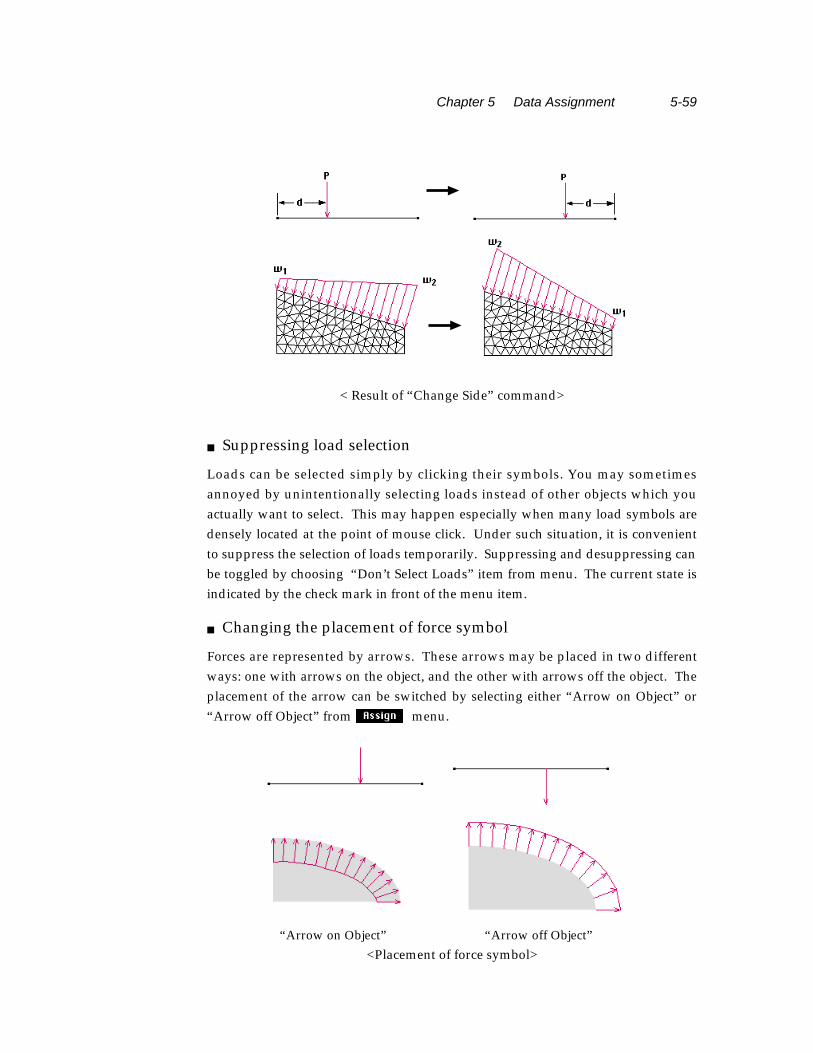
Chapter 5 Data Assignment 5-59
< Result of “Change Side” command>
■ Suppressing load selection
Loads can be selected simply by clicking their symbols. You may sometimes
annoyed by unintentionally selecting loads instead of other objects which you
actually want to select. This may happen especially when many load symbols are
densely located at the point of mouse click. Under such situation, it is convenient
to suppress the selection of loads temporarily. Suppressing and desuppressing can
be toggled by choosing “Don’t Select Loads” item from menu. The current state is
indicated by the check mark in front of the menu item.
■ Changing the placement of force symbol
F o rces are re p resented by arrows. These arrows may be placed in two diff e re n t
ways: one with arrows on the object, and the other with arrows off the object. The
placement of the arrow can be switched by selecting either “Arrow on Object” or
“Arrow off Object” from menu.
<Placement of force symbol>
“Arrow on Object” “Arrow off Object”

5-60 Chapter 5 Data Assignment
■ Limiting the size of force symbol
The size of the arrow re p resenting a force is determined to be appro x i m a t e l y
proportional to the magnitude of the force. When there are big differences in the
magnitudes of the forces, some of arrows become too large to be appro p r i a t e l y
drawn on the screen. For such circumstances, it is necessary to limit the size of
a r rows. This can be done by selecting “Limit Arrow Size” item from
menu.
■ Resetting the size of force symbol
As you continue assigning load conditions, the size of arrow may become
inappropriate, even though the load drawing scale can be adjusted using the slide
bar of "Load Condition" dialog. In such case, it is desirable to reset the default size
of the arrow by selecting “Reset Arrow Size” item from menu.

Chapter 5 Data Assignment 5-61
Load Combination
Multiple sets of analysis results can be obtained at once by solving a model
with multiple load cases. Each load case is defined by linear combination of
the load sets. A force vector Fr for the system equations is obtained by
linear combination of m force vectors, F1, ..., Fm, which may be expressed by
the following equation,
As many load cases as desired can be formed by various combinations of the
load sets, and can be used for independent analyses. Instead of solving the
equations with each one of the load cases, the program solves all the cases at
once, and thus saves the computing time significantly. The results fro m
various load cases can be combined further with desired factors to form a
new sets of analysis results.
The function of load combination is valid only for linear static analysis.
■ Defining load combinations
Load combination is meaningful only when there are 2 or more load condition sets
applied to the model. A load case is defined by combining all or parts of the load
sets with certain combination factors by the following factors.
1) Choose "Load Combination" item from menu.Then, "Load Combination" dialog appears on the screen.
2) Create or delete a combination set using or button in the
dialog.
combination factor C7
Check this button to includethe load set in the combination
load set number
inidicator of the current load set
Boxes of unassigned load setsare dimmed.
Fc = ciFii=1
m
∑

5-62 Chapter 5 Data Assignment
The usage of the dialog is similar to that of assignment dialogs except that
there is no button.
3) Check the load sets to be include in the combination.
Click the check boxes to turn on or off the inclusion of load sets in the
combination. Only the load sets applied to the model can be included in a
combination.
4) Insert the combination factors ci in the editable text boxes.
There appears an editable text box to the right of the included load set text.
Insert the text of the combination factor in the box. The factor can be either
positive or negative.
You may define as many load cases as necessary. However, it should be considered
that further combination of analysis results is also possible after solving the model
with multiple load combinations.
■ Handling load condition sets in "Load Combination" dialog
The "Load Combination" dialog may be displayed along with the "Load Condition"
dialog as shown in the figure below. You may change the current load set by
clicking the corresponding indicator in the "Load Combination" dialog.
Alternatively, you may also change the highlighted indicator by selecting a popup
menu(Windows:dropdown list) item in the "Load Condition" dialog.
<"Load Combination" dialog displayed along with "Load Condition" dialog>
■ Combining analysis results of multiple load conditions
The analysis results with various load combinations can be combined further as
described in Chapter 7.
popup menu to selectdynamic motion item
Turn on this buttonto assign transientdynamic motions
Click this buttonto start editinga transientmotion set.
current time step
current time
dynamic motionsin X, Y and Z directions

Chapter 5 Data Assignment 5-63
Dynamic Motions
Dynamic motions can be explicitly prescribed at nodes in dynamic analysis.
In order to start assigning dynamic motions, choose “Dynamic Motion” item
in menu. “Dynamic Motion” dialog pops up, and current state of
their assignment is displayed in the main window.
Dynamic motions can be applied to fixed degrees of freedom as well as to free d.o.f.
However, application of motion to fixed d.o.f. tends to increase the solution time.
Defining and assigning dynamic motion sets
Dynamic motions can be defined and assigned by the unit of data set similar to
load condition set. A dynamic motion set is initially created by clicking
button of “Dynamic Motion” dialog. If a dynamic motion set is already assigned,
additional assignment of the set, either to a single object or multiple objects,
creates a new set automatically by duplicating the original one.
The popup menu of "Dynamic Motion" dialog has the following items:
• "Displacement": transnational displacements assigned at nodes.
• "Velocity": transnational velocity assigned at nodes.
• "Acceleration": transnational acceleration assigned at nodes.
• "Nodal Dashpot": damping dashpot attached at nodes.
• "Nodal Mass": mass assigned to nodes.
The top 3 items correspond to types of dynamic motion and the other two to
dynamic resistance, which is described in the next section.
popup menu to selectdynamic motion item
Turn on this buttonto assign transientdynamic motions
Click this buttonto start editinga transientmotion set.
current time step
current time
dynamic motionsin X, Y and Z directions

5-64 Chapter 5 Data Assignment
■ Setting the time dependency of dynamic motion
The time dependency of dynamic motion can be set as one of the 3 types, harmonic
transient and initial types. In order to set the time dependency, click the
c o r responding radio button, "Harmonic", "Transient". or "Initial" in "D y n a m i c
Motion" dialog. As you alter the option of time dependency, you will notice the
changing items below the radio buttons. Time dependent variation of dynamic
motions is defined and modified using these items.
■ Defining harmonic motions
A harmonic motion has periodic characteristics with changing magnitudeexpressed by a sinusoidal function . The dynamic motion acting at a
specific time is obtained by multiplying the function by the amplitude of motion
given at the bottom of the dialog.
Click "Harmonic" radio button to define a set of harmonic motions. The
amplitudes of the motion components are defined by inserting the values in the
editable text boxes of motion components.
■ Defining transient motions
A transient motion is defined by a series of values at a number of time steps,
which can be created and edited by the following steps.
1) Select an item of dynamic motion from popup menu in “Dynamic Motion”
dialog.One of "Displacement", "Velocity" and "Acceleration" items should be selected.
2) Turn on “Transient” radio button in the dialog.Then, the items below the radio buttons take on the appearance shown at the
starting timeof application
ending timeof application
sin t − to( )
maximum amplitude of motion
sin t − to( )

Chapter 5 Data Assignment 5-65
beginning of this section ("Dynamic Motion"). They include the current step
number and the current time. The current time step can be edited by directly
changing the number in the box, or by scrolling the number.
3) Click button.
Then, "Dynamic Motion Series" dialog pops up. The dialog pro d u c e s
editable data items for each time step you create. The data items are
equivalent to the data items in "Dynamic Motion" dialog.
4) Click button to add a time step.A line of data items will be created for the new time step. In order to delete a
time step, click button after selecting the corresponding data line.
5) Select a line or a cell to edit.Then, the data on the line or in the cell will be reflected in the editable text
boxes at the bottom of the dialog
6) Edit the text in the editable text box.As you edit the text in a text box, it will immediately be echoed in the actual
data line.
7) Click button after completing creation of time steps."Dynamic Motion Series" closes and the data from the dialog are
automatically reflected in "Dynamic Motion" dialog.
The data on the last line are assumed to be maintained up to the last time step in
the analysis.

5-66 Chapter 5 Data Assignment
■ Defining initial motions
Initial motions are used to define the initial state of the analysis at time 0. The
type of initial motion is either displacement, velocity or acceleration. Click "Initial"
radio button of the "Dynamic Motion" dialog to define and assign initial motions.
■ Assigning dynamic motions
Dynamic motions can be assigned to various types of objects including nodes,
curves, surface meshes or volume meshes. However, they are eventually assigned
to nodes contained in the assigned objects. You should first choose the selectiontool, , , or in order to assign the dynamic motion sets to objects of
desired type.
Defining and assigning nodal dynamic properties
As described in the previous section, the popup menu of "Dynamic Motion" dialog
has items other than dynamic motion itself. They are concerned with dynamic
p roperties assigned at nodal points. "Nodal Dashpot" is to assign damping
characteristics to nodes, and "Nodal Mass" is to assign concentrated mass to nodes.
A nodal dashpot is a damper decelerating nodal movement, and nodal mass
carries inertia force conceptually concentrated at nodal points.
■ Nodal dashpot
Nodal dashpot represents a damper attached to a node. A nodal dashpot can be
defined and assigned by the following steps:
1) Select "Nodal Dashpot" item from popup menu in “Dynamic Motion” dialog.The editable text items on the dialog turn into states for defining a damping
coefficient for each nodal d.o.f.
2) Insert values into the editable text items.A damping coefficient is specified independently for each nodal d.o.f. For
example, Cx, Cy, and Cz a re damping coefficients for 3 nodal d.o.f in 3-D
solid case.
3) Select nodes or objects containing the nodes to assign the nodal dashpot..
4) Click button in the dialog.The nodes assigned with the dashpot are marked by red rectangle.

Chapter 5 Data Assignment 5-67
<Conceptual diagram of nodal dashpot>
■ Nodal mass
A nodal mass is a mass conceptually concentrated at a node, which makes the
nodal movement produce inertia force or moment. Nodal mass can be defined and
assigned by the following steps:
1) Select "Nodal Mass" item from popup menu in “Dynamic Motion” dialog.
The editable text items on the dialog turn into the state to get nodal mass
components defined for each nodal d.o.f.
2) Insert values into the editable text items.
The conceptual nodal mass is specified independently for each nodal d.o.f.
For example, mx, my, mz, mrx, mry, mrz are mass components for 6 nodal d.o.f
in 3-D frame model. The latter 3 are rotary inertias.
3) Select nodes or objects containing the nodes to assign the nodal mass..
4) Click button in the dialog.
The nodes assigned with the nodal mass are marked by red rectangle.
<Conceptual diagram of nodal mass>
nodal mass my
acceleration ay(t)
inertia forceFy(t) = my ay(t)
damping coefficient Cx
damping force Fx(t) velocity of nodal movement vx(t)
nodal dashpot
Fx(t) = Cx vx(t)

5-68 Chapter 5 Data Assignment
Frame Member Joint Conditions
Frame member joint conditions are meaningful only for 2-D and 3-D frame
analysis. Frame members are basically connected rigidly with other
members at their joints. But some of them may be pin- jointed. The state of
member connection can be defined as member joint condition sets and
assigned to corresponding members.
In order to start assigning member joint conditions, choose “Element Joint”
item from menu. Then, “Member Joint” dialog box appears on the
screen.
Defining frame member joint conditions
The frame member joint conditions are defined as a data set using “Member Joint”
dialog. There are only two data items, each of which represents the joint condition
at one end of a frame member. It is assumed that each frame member has only two
end nodes: the left and the right end node. The check mark of the check box in
front of “Left end node” or“Right end node” indicates that the corresponding node
is pin-jointed. The check mark is turned on and off by clicking the check box. In
order to define a truss member joint, turn on both check boxes. Unchecking both
of the check box makes the member joint condition with both ends rigidly jointed.
Defining such a joint condition is redundant, because all the frame members are
originally assumed to be rigidly jointed at both of their ends.
Assigning frame member joint conditions
In order to assign the currently active member joint condition set, first select the
m e m b e r, and click button of the dialog . The member will get the joint
condition defined by the set, and will be marked in red colors. The pinned joint is
also marked in the drawing of the member as shown below.
<Representation of member connectivity>
Both ends are rigidly jointed. One end is pin jointed. Both ends are pin jointed.
pin-connected at the left node if checked
pin-connected at the right node if checked

Sequentially Staged Modeling
Sequentially staged modeling is devised for analysis of objects with
changing geometry, material properties and load conditions over a given
period of time. Such a modeling is useful in analyzing structures like dams,
tunnels and bridges under construction. The sequentially staged modeling
option is turned on by checking the "Sequential" button of the "Pro j e c t
Setup" dialog. (Refer to "Project and File" section of Chapter 1.) The menu
item, "Sequential Stage" of menu is enabled when this modeling
option is turned on.
The "Sequential Stage" dialog can be toggled between the expanded and
s h runken states using the toggle button. The dialog is in the expanded
state, and turns to the shrunken state automatically when an assignment
dialog (such as "Property" or "Load Condition" dialog) is opened.
Chapter 5 Data Assignment 5-69
stage number popup
stage label
button to exclude the selected objectsfrom the current stage
button to include the selected objectsin the current stage
to show all objects in the model
to show all objects in the last stage
to show objects included at the current stageto show objects excludedat the current stage
to show all objects in the next stage
to show all objectsin the current stage
option to use the assumed stressfield for the current stage
option to relax the stresses due tounbalanced forces at the predefined
rates over the next few stages
option to clear the displacements but retainthe stresses computed at the current stage
the time of the current stage(used only for coupled analysis)
button to set the assumedstress field
button to set the schemeof stress relaxation
expand/shrink toggle button
< expanded state >
< shrunken state >

5-70 Chapter 5 Data Assignment
In order to start defining and assigning the sequential stages, choose "Sequential
Stage" item from menu. Then, "Sequential Stage" dialog opens as shown
b e l o w. The model of each stage is created by using this dialog. Usage of the
dialog items is explained below.
Click this button to create a new stage and display the state of the new
stage. The new stage model initially inherit its contents from the last
stage model or from the base model.
The current stage is deleted by clicking this button. The next or the
previous stage becomes the current stage.
The current stage number is displayed as a popup menu(Wi n d o w s :
drop-down list) item. You may move to the desired stage using this
popup menu (Windows: drop-down list).
The label of the current data set. You may label a data set by entering
a character string in the text box.
This button is used to scroll up the stage. The current stage is scrolled
up by this button. Clicking this button once reduces the current stage
number by one.
This button is used to scroll down the stage. The current stage is
scrolled down by this button. Clicking this button once increases the
current stage number by one.
The point of time for the current stage. This item is used only for
structural analysis coupled with transient seepage -analysis.
Expand/shrink toggle button. Click this button to expand or to shrink
the dialog.
Click this button to include the selected objects into the current stage
model. If the selected objects are already included in the current stage
model, this button is dimmed.
Click this button to exclude the selected objects from the current stage
model. If the selected objects are not included in the current stage
model, this button is dimmed.
If this radio button is on, all the objects, i.e. the objects of the base
model are displayed. Click this button to show all objects of the base
model independent of the stages.
Click this button to display the previous stage model.
Click this button to display the current stage model.
Click this button to display the next stage model.
Click this button to display the objects included at the current stage,
i.e., the objects which are not in the last, but in the current stage
model.
Click this button to display the objects excluded at the current stage,
i.e., the objects which are in the last, but not in the current stage
model.

Concept of sequentially staged modeling
Stage is a core concept of the sequentially staged modeling. This section describes
the finite element procedures based on the stages, and the inter-relation of analysis
results and modeling data between stages.
■ The base model and the stage models
A sequentially staged model consists of 2 or more stages. Each stage has all
i n g redients of finite element analysis by itself and is modeled to re p resent the
actual situation with changing geometry, properties, and load conditions. The
finite element analysis model for a stage is termed here as "stage model", while the
model with all data shared by all stages are termed as "base model." A sequentially
stage modeling always involves one base model and 2 or more stage models.
The base model is displayed on the screen when the "Sequential Stage" dialog is
not shown. The stage model of the current stage is displayed when "Sequential
Stage" dialog is opened. You can move to the desired stage either by using the
stage number popup menu(Windows: dropdown list), or by using the scro l l
buttons. The current stage number appears as the popup text. The current stage
can also be identified by the label displayed in the label text box. The geometry,
properties, boundary conditions and load conditions of the current stage model is
displayed in the main window if the dialog is opened and the display mode is set
to "Current". At the moment you close the dialog, the display on the main
window returns to the base model.
Chapter 5 Data Assignment 5-71
stage model“Sequential Stage” dialog is not shown.base model
The current stage number is shown in “Sequential Stage” dialog.
<Base model and stage model>

■ Data sharing and inheriting
All the stage models share the data of the base model. In other words, the base
model comprises all the data included in the stage models. The first created stage
model (the stage model of stage 1) initially inherits its data from the base model,
and is later modified to keep only necessary data by using exclusion, assignment or
clearing actions. Likewise, a subsequent stage model initially inherits its data from
the preceding stage model, and is modified later by various actions.
Creation or modification of geometric objects, i.e., curves and meshes are allowed
only for the base model. Thus, new objects cannot be attached to a stage model
d i re c t l y. The geometric objects created for the base model are automatically
inherited to all the currently existing stages.
On the other hand, properties and load conditions can be assigned directly to a
stage model. Any assignment performed at a stage level is applied to the
c o r responding stage model, and also included in the base model. But the
assignment is not applied to the other stage models. Nevertheless, any assignment
to the base model is automatically inherited to all the currently existing stages.
5-72 Chapter 5 Data Assignment
<Concept of data sharing and inheriting>

Chapter 5 Data Assignment 5-73
■ Solution process of stage models
A complete processing of finite element solver is performed for each of the stage
model. The processes are repeated, starting from the first stage and pro c e e d i n g
sequentially to the last. Each process of a stage model is not independent from the
others. A stage model is processed in association with its preceding or subsequent
stage. The solution results of a stage model are reflected in the processing of the
next stage model. For example, unbalanced forces resulting from excavation at a
stage are relaxed over the next few stages with prescribed rates. The solution
results such as displacements, stresses and so on are accumulated stage after stage.
The data accumulation can be artificially controlled if necessary. As an example,
the nodal displacements are cleared at the first stage while the computed stresses
a re retained, which is usually applied to modeling construction stages in
consolidated soil.
■ Procedure of sequentially staged modeling
A stage model is constructed in the form of extracting necessary components from
the base model. The pr o c e d u re of sequentially staged modeling can be
summarized as follows:
1) Create the base model.It is recommended to complete creating the base model before creating the
stages, although the base model may be added or modified in the middle of
working with stage models.
2) Create stage models and build the geometry of the stage models.The geometry of a stage is constructed initially by inheriting the geometry
f rom the base model or from the previous stage, and then modified by
"Include" and "Exclude" actions.
3) Build the data assignment of each stage model.P roperty and load condition data of a stage is constructed initially by
inheriting the data from the base model or from the previous stage, and then
modified by assigning or clearing data.
4) Execute the solution process.
The finite element solution process is launched in the same way as non-staged
models. Select "Solve" item of menu to go through the solution
p rocess. (Refer to "Processing of structural analysis" section of Chapter 6.)
However, a complete solution process is repeated for each of the stages. The
analysis results of a stage are accumulated and applied as a part of input data
for the analysis of the subsequent stages.
5) Postprocess the analysis results.
The analysis results of the staged model are arranged and saved as a
sequential process. The visualization of the analysis results can also be
controlled sequentially in accordance with the staged progress.

5-74 Chapter 5 Data Assignment
Creating stage models
Sequentially staged modeling is initiated by choosing "Sequential Stage" button
from menu. Stage 1 exists at the beginning of staged modeling. Stage 1
initially includes all the objects created so far, and the current assignment of
properties, boundary conditions and load conditions.
■ Creating a new stage
A new stage is added to the staged model by clicking button. If the current
stage is the last one, the new stage is attached to the last. If the current stage is not
the last one, the new stage is inserted between the current and the next stage.
A c c o rd i n g l y, the next and the following stages are reassigned with subsequent
numbers.
The new stage model initially inherits the geometry and the attributes from the
current stage which is now stated as previous stage. The newly created stage takes
the status of current stage.
■ Deleting a stage
The current stage is deleted by clicking button. If the current stage is the
last one, the previous stage takes the status of current stage. Otherwise, the next
stage takes the status of current stage, and the subsequent stages are renumbered
a c c o rd i n g l y. There should be at least one stage, and there f o re the current stage
cannot be deleted if there is only one stage.
■ Moving to the desired stage
You can move to the desired stage either by using the stage number popup
menu(Windows: dropdown list), or by using the scroll buttons. The current stage
number appears as the popup text. The current stage can also be identified by the
label displayed in the label text box. the contents of the main window, i,e.,
g e o m e t r y, properties, boundary conditions and load conditions are displayed on
the basis of the current stage.
Building the geometry of stage models
In a sequentially staged modeling, each of the stages represents a complete model
with all ingredient of finite element analysis, composed of geometry, pro p e r t i e s ,
boundary conditions and load conditions. However, it is not necessary to create
independent models for the stages. Instead, a stage can be constructed simply by
including and excluding its components from the predefined base model.
■ Including the selected objects to the current stage
It is the case in which the objects not in the previous stage is to be included into the
Chapter 5 Data Assignment 5-75
current stage. Before including the objects into the current stage, they may not be
displayed at the current stage depending on how the display option is set. In order
to make the desired object visible, check "All" or "Last" radio button. Then, select
the object, and click button. If the selected objects are already within the
current model, the button is dimmed.
■ Excluding the selected objects from the current stage
It is the case in which the objects in the previous stage is to be exclude from the
c u r rent stage. Select the objects to exclude, and click button. If the
selected objects are not within the current model, the button is dimmed.
■ Handling objects created after creation of some stages
As mentioned previously, it is desirable to complete the creation of the base model
and then to start creating the stages. Owing to some reason, however, a part of the
base model might have been created after creation of some stages, all or in part. In
such situations, the newly created objects are automatically included into all the
stages already created. If unwanted objects are included in this way, you should
move to the relevant stage, and exclude the objects manually.
■ "Model Display" options
Only displayed objects are selectable, and thus can be included or excluded as
d e s i red. There f o re, it is necessary to control the state of visibility of the desire d
objects for building the geometry of a stage. The "Sequential Stage" dialog has
radio buttons, "All", "Previous", "Current", "Next", "Included" and "Excluded" for
the option of object display. The usage of the buttons is described at the beginning
of this section.
Property assignment in sequentially staged modeling
In a sequentially staged modeling, the property assignment also varies with stages.
For example, a surface mesh region is assigned with property set A at stage 1, and
the property of the same region is altered to set B at stage 2. This is the case of a
c o n s t ruction modeling with changing material property in some part. Pro p e r t y
assignment can be handled either collectively by working with the base model or
individually by working with a stage model.
In order to start property assignment, select "Structural Property" item fro m
menu. If the "Sequential Stage" dialog is not currently on, the property
assignment is performed for the base model. If the dialog is already opened, the
dialog shrinks, and the "Structural Property" dialog is positioned at the bottom of
the "Sequential Stage" dialog as shown in the figure below. In this case, the
assignment is applied to the current stage model.

5-76 Chapter 5 Data Assignment
■ Assigning properties to the base model
The base model takes the property assignment and deletion, when "Sequential
Stage" dialog is not on. And the assignment to the base model is automatically
inherited to all stage models which have the assigned objects. Deletion of a
property set in the base model is also applied to all stage models. Thus, property
assignment or deletion in the base model overrides the previous assignments in all
stage models at once.
<Property assignment of the base model>
■ Assigning properties to stage models
Only one property set can be applied to an object in the base model, although the
property of an object can be altered from one stage to the other. Assignment of the
changing properties can be achieved by assigning diff e rent property sets to the
stage models. The current stage model takes the property assignment and
deletion, when "Sequential Stage" dialog is on. The current stage is indicated by
the popup menu item in the dialog. Property assignment to a stage model does
base model
stage 1 model stage 2 model stage 3 model stage 4 model
property assignmentor deletion
inherited to all stage models
“Sequential Stage” dialog is shrinked.
Assignment is applied to the base model. Assignment is applied to the current stage model.
base model stage model
< Property assignment to the base model and to a stage model >

not affect the assignment of other stage models. However, the assignment is
registered in the base model.
<Property assignment of a stage model>
Load assignment in sequentially staged modeling
Load assignment can be handled either collectively by working with the base
model or individually by working with a stage model. It is similar to the case of
property assignment. The load assigned to the base model is inherited to the stage
model. However, in solving the whole staged model, a load assignment to an
object is effective only for one stage model. In the case of assignment with the
base model, the load set is effective at the stage in which the assigned object first
appears. In the case of assignment with a stage model, the load set is effective at
that stage only.
Assignment of load conditions is initiated by selecting "Load Condition" item from
menu. If the "Sequential Stage" dialog is not currently on, the load
assignment is performed for the base model. If the dialog is already opened, the
dialog shrinks, and the "Load Condition" dialog is positioned at the bottom of the
"Sequential Stage" dialog as in the case of property assignment.
■ Assigning loads to the base model
A load condition applied to the base model is inherited to stage models. This does
not mean that the load condition is applied to all stage models, but means that the
load takes effect at one of the inherited stage models in which the assigned object
appears for the first time. Each of the load conditions is involved only once in the
system equations, and it is the system equations at the stage the load takes effect.
Thus, actual application of the load conditions in the base model is determined
automatically by the program, and cannot be controlled by the user.
The following example illustrates how the load assignment of the base model takes
effect in stage models. Load 1 to 4 are applied to the base model. Load 4 becomes
effective at stage 1, because the object assigned with the load is already in the stage
model. Load 2 and 3 take effect at stage 3 in which the assigned object appears.
Finally, load 1 appears at stage 4.
base model
stage 1 model stage 2 model stage 3 model stage 4 model
property assignmentor deletion
registered in the base models
Chapter 5 Data Assignment 5-77

5-78 Chapter 5 Data Assignment
■ Assigning loads to stage models
A load condition applied to the base model takes effect at the stage the assigned
object appears first. Thus, the stage of actual application may not be realized as
desired. Such a problem can be solved by assigning the load condition directly to
the desired stage. The following figure shows an example illustrating the
difference between the load assignment to the base model and the assignment to
the stage models.
base model
stage 1 model stage 2 model stage 3 model stage 4 model
load 1
load 2
load 3
load 4
load 4
load 1
load 3
load 2
base model
<Load assignment to the base model>
<Load assignment to stage models>

Control in processing of a sequentially staged model
The solution results of a stage model and their reflection on subsequent stage
models can be artificially controlled to embody the actual situation more
realistically.
■ Assumed stress field of a stage model
The solution results of a stage model can be replaced by assumed stress field as a
whole or in part. Such a fabrication of the analysis results is often used to
represent the initial state in soil mechanical analyses.
If you check the "Assumed stress field" box, button to the right turns to
enabled state from disabled state. Click the button to designate how the stress field
should be assumed. Then, "Assumed Stress Field" dialog appears.
Using the dialog, the stresses can be controlled as follows:
• "Vertical Direction": Select the vertical direction from the coordinate axis, X,
Y and Z . This option is enabled only for 3-D problems. The Y direction is
assumed to be the vertical direction for 2-D modeling.
• " Vertical Stresses": Select the way how the stresses in the vertical dire c t i o n
should be determined. If "As solved" ratio button is on, the vertical stresses
a re determined by the finite element solution. Otherwise, the vertical
stresses are directly calculated from the vertical loads.
• "Horizontal Stresses": Select the way how the stresses in the horizontal plane
should be determined. If "Vertical Stress × Ko" option is on, the horizontal
s t resses are directly calculated from the vertical stresses using the neutral
soil pressure coefficient Ko.
Chapter 5 Data Assignment 5-79
coordinate axis designated as the vertical direction
options specifying the vertical stress field
options specifying the horizontal stress field
options specifying the shear stress field

5-80 Chapter 5 Data Assignment
• "Shear Stresses": Select the way how the shear stresses should be
determined. If "Ignore" option is on, the shear stresses are set to 0,
regardless of the actually computed values.
In order to nullify the rule of stress assumption and use the solved values, uncheck
the "Assumed stress field" box.
■ Prescribing the staged stress relaxation rate
Excavation during construction can be modeled simply by excluding the elements
of the excavation part from the corresponding stage model. Removal of elements
results in change of stresses. In sequentially staged analysis, it is sometimes
assumed that the stress change does not occur at once, but gradually over a few
stages. Such an assumption is often adopted in 2 dimensional modeling of
excavation pro g ressing in the direction vertical to the plane. The assumption is
based on the concept of unbalanced forces and stress relaxation. At the beginning,
t h e re exist unbalanced forces resisting the stress change. Stress relaxation, i.e.,
transition of stresses to the final state progresses gradually in accordance with the
reduction of the unbalanced forces.
< Concept of unbalanced forces and stress relaxation >
The gradual stress transition is represented by the stress relaxation rates prescribed
for the stages subsequent to the excavation. The procedure of prescribing the stress
relaxation rates is as follows:
1) Check "Stepwise stress relaxation" box in the "Sequential Stage" dialog.
Only when the box is checked, button to the right is enabled.
Otherwise, it is disabled.
2) Click button to open "Stress Relaxation Rate" dialog.
The stress relaxation rate is prescribed using this dialog.
3) Create the lines of stages by clicking button.
The stage offset indicate the number of stages from the current stage. The
offset of the current stage is 0. Create as many stages as the relaxation rate is
prescribed.
4) Set the relaxation rates.
vertical stress due to body weightbefore excavation
stress after excavationwithout unbalanced forces
(100% stress relaxation)
stress after excavationwith full unbalanced forces
(0% stress relaxation)

Set the relaxation rate for each lines of stages. There are 2 columns of
relaxation rates. "No Refilling" column prescribes the relaxation rates of
excavation without refilling. "w/ Refilling" column applies to the relaxation
rate of excavation with later refilling.
4) Click button to complete prescribing the stress relaxation rate.
The relaxation rate data is saved to a text file by clicking button, and
imported from a text file by clicking button.
■ Clearing displacements
T h e re is an option to clear all the displacements accumulated up to this stage.
Check "Clear displacement" box to remove the displacements but retain the
stresses. This option is often used at the initial stage of soil mechanical analysis to
represent the initial state of stresses due to body weight.
Chapter 5 Data Assignment 5-81
stage elapse =1
70% stress relaxation(30 % unbalanced forces)
currentstage
number of stages from the current stage
time from the current stage
stress relaxation rate for excavation without refilling
stress relaxation rate for excavation with refilling
adda new line
delete theselected line
save the data in a text file read the data from a text file
pre-excavation stage
stage elapse =0(excavation stage)
40% stress relaxation(60 % unbalanced forces)
stage elapse =2
100% stress relaxation(0 % unbalanced forces)
< Prescribing the stress relaxation rate >

5-82 Chapter 5 Data Assignment