chapter 5 product differentiation versus …...with differentiation, where price or product choice...

157

Kumagai, Satoru, ed. 2010. New Challenges in New Economic Geography. Chiba: Institute of Developing

Economies.

Chapter 5 Product Differentiation versus Geographical Differentiation: Evidence from the Pork Processing Industry in China

Mariko WATANABE◎

Abstract

This chapter attempts to identify whether product differentiation or geographical

differentiation is the main source of profit for firms in developing economies by

employing a simple idea from the recently developed method of empirical industrial

organization. Theoretically, location choice and product choice have been considered as

analogues in differentiation, but in the real world, which of these strategies is chosen

will result in an immense difference in firm behavior and in the development process of

the industry. Development of the technique of empirical industrial organization enabled

us to identify market outcomes with endogeneity. A typical case is the market outcome

with differentiation, where price or product choice is endogenously determined. Our

original survey contains data on market location, differences in product types, and price.

The results show that product differentiation rather than geographical differentiation

mitigates pressure on price competition, but 70 per cent secures geographical monopoly.

Keywords: Product differentiation, geographical differentiation, price competition JEL Code: O14, O53, L13, L11

◎ Corresponding author: Institute of Developing Economies, JETRO, Chiba. This is an incomplete version. Please do NOT quote.

158

1. Introduction: Geography or Product for Promoting Development?

What kinds of behavior by firms lead to what types of economic development? In order

to consider this question, this chapter is motivated to identify what kinds of competition

strategies firms adopt and produce profit. Firms are always under pressure from

competition which may reduce their profit to zero or a negative figure. In order to avoid

this outcome and to survive, firms will adopt a strategy of differentiation. Entrepreneurs

and firms focus on how to make themselves different from others. Once differentiation

strategies are set, firms will start allocating internal resources and shaping their

organization. Their strategy will determine how they behave and how they look, and it

may affect demand for substantial factors such as labor, capital and the profile of the

development process of the economy.

Sources of differentiation are extremely diversified because this diversity is the

source of survival of firm. In this chapter, we examine product differentiation and

geographical differentiation as two competing strategies. Differentiation in product is a

well known strategy, particularly among Japanese industry. To succeed in differentiation

of products, a firm needs certain capabilities, for example, precise research on

consumers‟ preferences, research and development to produce new products, and an

acute sense of style to give „trendiness‟ to their products or services. In contrast, if firms

have successfully differentiated geographically in an industry, the firms‟ products may

be quite homogenous because firms have little or no incentive to differentiate. Due to

the smaller requirements for production technology in the case of geographical

differentiation, firms in developing economies may prefer to adopt this strategy.

However, the development of distribution technology or retail strategies may reduce the

success of geographical differentiation. This chapter is motivated to present evidence on

159

what kinds of strategies have been adopted and have benefited the firms in the „real

world‟ as a means of considering what kinds of strategies by firms may lead to what

types of economic development.

This chapter is organized as follows. Section 2 reviews the literature on

empirical methods which are undergoing extraordinary development in industrial

organization studies. This development is likely to be strongly connected with spatial

economy. Section 3 describes the background of this research, the dataset to be used and

basic observations from the data. Section 4 reports on the structural model, estimation

strategy and results. Section 5 discusses the extant problems and presents the

conclusion.

2. Literature Survey

To identify the “source of differentiation,” we need a method of estimation for an

endogenously determined market structure. The recent development of structural

estimation enables us to capture the outcome of strategic interaction. According to

Reiss and Wolak (2007), structural estimation can be defined as an approach that

economic model is used to develop mathematical statements about how observable

“endogenous” variables are related to observable and unobservable “exogenous”

variables. By doing this, researcher can estimate unobserved economic or behavioral

parameters that could not be otherwise inferred from non-experimental data1. This

approach is developing in a field called empirical industrial organization. In particular,

research on two strands, estimations of demand system and estimation on decision to

1 Experimental data can allow the researchers to infer structural estimates, but structure that economic theory provide will give more clear relationship with experimental data.

160

enter a market are accumulating.

If one focuses on a demand system where the products are differentiated and

prices are set accordingly, you have to deal with the problem that price is not exogenous

to the consumer‟s decision but rather is endogenous because the firm will set prices

according to the expected preference of the consumer. Price is an endogenous variable.

Use of an instrument variable to price may be the first idea to hit, but it is not easy to

find good instruments that represent the heterogeneous preferences of all consumers in

the market. Berry (1994) pointed out that the constants can be included in the choice

model by the consumer to capture average effect of product attributes which are most

likely unobservable. Berry (1994) and Berry, Levinson and Pakes (1995) demonstrated

that by transforming the market shares into a function of the unobservable product

attributes that generates endogeneity on price, unobservable attributes appears as a

linear term. By doing so, a traditional instrumental variable estimation becomes feasible.

This approach forms a major strand of empirical industrial organization (see Nevo 2001,

Train 2003: Chapter 13 ) In order to deal with endogeneity of price-product choice, it

may help to conduct an experiment to obtain information on consumers‟ preferences

(see Train 2003).

If one is focusing on the decision to enter a certain market, there again occurs

the endogeneity problem. In a standard setting, firms will decided to enter a certain

market when they expect profit, and this behavior is estimated by a discrete choice

model such as probit. Among structural variables in the profit function, selling price and

marginal cost are subject to strategic behavior and may become endogenous. If the price

of a firm‟s products depends on number of rivals, firm‟s decision on entry to a market

may affect the price. Particularly in oligopolistic environment, the number of rivals is

161

the outcome of strategic interaction among the potential entry firms and consists of

essentially endogenous variables. Another problem is that the equilibrium of this entry

game could be multiple and not unique.

Berry (1992) dealt with this problem by taking numbers of firms in the market

as a target of estimation in the flight route market of the airline industry in United States.

Jia (2008) dealt with this problem by transforming a profit maximization problem into a

search for the fixed points of the necessary conditions in capturing Walmart, K-mart and

small retailers in 2,065 counties. This model allows for flexible competition patterns

among all players. Seim (2006) employed a nested fixed-point algorithm solution in

estimating the model for location choices in the video retail industry. Mazzeo (2002)

proposed a two-stage estimation procedure à la Hekit in estimating the effect of market

concentration and product differentiation in an observed configuration of high and low

quality types in the motel industry. This chapter employs Mazzeo‟s (2002) two-step

approach.

Marginal cost, too, may become a source of endogeneity in an entry model.

This happens when the marginal cost may be reduced when the firm decides to enter.

This actually happens in a case of the chain store market, where a large chain may

benefit by reducing distribution cost or advertisement cost when it sets off a „chain

effect,‟ by its decision to enter. Jia (2008) succeeded in capturing this effect.

In relation to spatial economy, the problem of location choice has an affinity

with the later literature concerning the entry decision model. Theoretically, product

choice and location choice have been considered as analogues in differentiated markets

since Hotelling (1929). (See Andersen, De Palma, JF. Thisse 1992, Tirole 1988).

Empirical studies on location choice and spatial competition emerged in the 2000s,

162

benefiting from development of the empirical method of endogenous market outcome.

Regarding spatial competition, in addition to Jia (2008) and Nishida (2008) that

applied a similar approach to a dataset on convenience stores‟ network building choices

in Okinawa, Japan, Davis (2006) and Smith (2004) are conducting estimation on spatial

competition. However, the latter two researches take the firm‟s location as given, then

estimate quantity or price competition. Pinske, Slade and Brett (2002) proposed a

semi-parametric approach to spatial price competition.

3. Background of Case Study on Pork Processing Industry 3.1 Background

Pork is one of the most important foods for the Chinese. The industry is currently

undergoing a major transition, as prices and quality are now being questioned. In 2007,

pork prices skyrocketed in China nationwide, increasing about 70% over the previous

year. The direct cause of this price hike was an outbreak of blue-ear pig disease which

attacked sows heavily in 2006. The industry was vulnerable to this shock, and

production volume decreased drastically. A substantial portion of the production of pork

still relies on individual farmer‟s backyard production; due to rapid economic growth,

the opportunity cost of hog production for these farmers rose rapidly, and they easily

abandoned hog production and investment in sows. In addition to direct shock of the

disease, the high opportunity cost for farmers led to exaggerated shrinkage of pork

production.

As concerns about quality arose, this scattered backyard production system was

condemned again. The system made it difficult to conduct effective quality control, and

the ill-motivated farmers fed poisonous fattener feed to their pigs, which triggered

163

several the toxic and fatal accidents in 2006. Despite these concerns which the scattered

production system has generated, it has persisted so far. Could this be attributable to the

nature of competition in the market? Strategies to earn profit may shape the production

system both inside and outside of firms. So, identification of the source of profit and the

impact of pricing of products became a focal point of the research and led to the launch

of this study.

3.2 Data

The research described herein relied heavily on a unique survey conducted by the author

and her colleagues. This section describes the data.

3.2.1 Data sources

The data on pork processing market was obtained from an original survey conducted in

Jilin and Henan provinces in 2008 by the Institute of Developing Economies, Japan, and

the Chinese Academy of Agricultural Science.2 The target of the survey was pork

processing firms. The survey is unique in that it was designed to capture characteristics

of transactions between the surveyed firms and their customers and suppliers.

Demographic data such as population and fiscal expenditure of the county or city are

obtained from „Guidebook to the Administrative Zone of the People‟s Republic of

China,‟ and fiscal expenditure, a proxy of economic activity size, is from „Yearbook of

Fiscal Data at the County Level.‟

3.2.2 Data description

The dataset contains information on the characteristics of transactions and in both sales

2 Mariko Watanabe of IDE, Jimin Wang of CAAS and Sachiko Miyata of the World Bank designed the surveys and conducted a pilot survey. The entire survey was conducted with the cooperation with local statistics bureaus.

164

and procurement. In this chapter, a market is defined as the administrative area in which

the buyer is located, such as a particular city, ward, county or village. We have

information on demographics and market structure, i.e., the number of competitors, as

well. Samples were taken by asking firms to describe characteristics of transactions with

a specific partner, not with the market as a whole.

The hog production industry in China roughly flows as follows: Farmers raise

the piglets into pigs, middlemen pick up the pigs and transport them to the pork

processing firms, and then the firms distribute them to the wholesalers, retailers or the

wet market, or directly to the final consumer. Our survey focuses on the pork processing

firms because they are an unavoidable link in the industry flow since the Chinese

government permits only licensed processing firms to process pigs into pork as well as

because they have substantial bargaining power in the flow. The structure of the

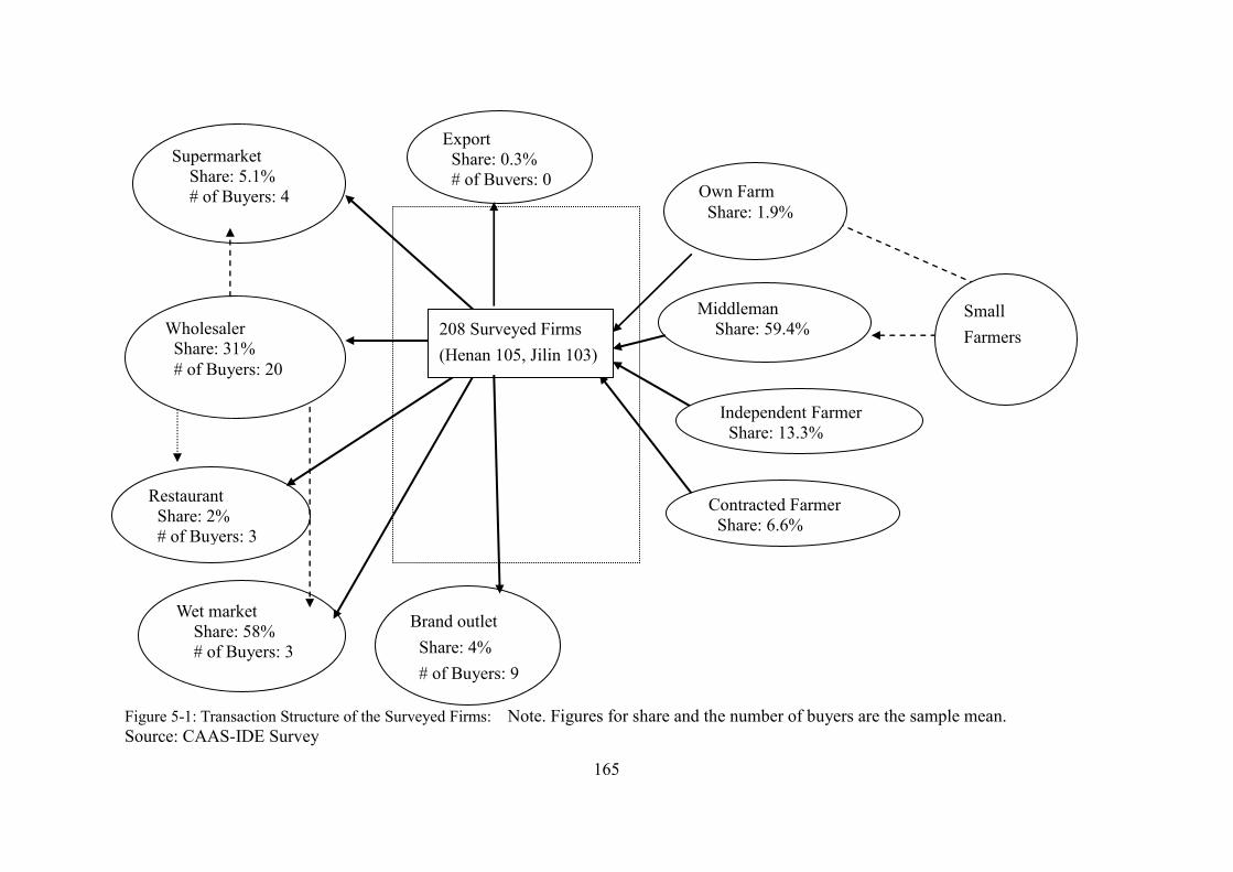
transaction flow captured by our survey is depicted in Figure 1. The functions filled by

the processing firms are as follow: (1) purchasing pigs, (2) slaughtering them (Raw

whole body pork will be sold to the customers at this stage. All processing firms fill this

function, and some processing firms focus only on this process.), (3) cutting into pieces

and cleaning, (4) selling and transporting in a chilled, controlled environment as „chilled

cut‟ pork, or (5) freezing and selling to the customers as „frozen cut‟ pork (Some

processing firms engage in this process.) and (6) cooking the pork into products such as

hams or boiled pork with soy sauce, etc. (Some firms do this in-house.). The pork from

(6) is sold as „cooked products.‟ The dataset contains „cooked products,‟ but the number

is very limited and the characteristics of products are similarity of products is more

further to other three types consisting of „raw whole body,‟ „frozen cut,‟ and „chilled cut.‟

Thus, the estimations in this chapter omit „cooked products.‟

165

Figure 5-1: Transaction Structure of the Surveyed Firms: Note. Figures for share and the number of buyers are the sample mean. Source: CAAS-IDE Survey

Own Farm Share: 1.9%

Small Farmers

Supermarket Share: 5.1% # of Buyers: 4

Restaurant Share: 2% # of Buyers: 3 Wet market

Share: 58% # of Buyers: 3

Wholesaler Share: 31% # of Buyers: 20

Middleman Share: 59.4%

208 Surveyed Firms (Henan 105, Jilin 103)

Export Share: 0.3% # of Buyers: 0

Brand outlet Share: 4% # of Buyers: 9

Contracted Farmer Share: 6.6%

Independent Farmer Share: 13.3%

166

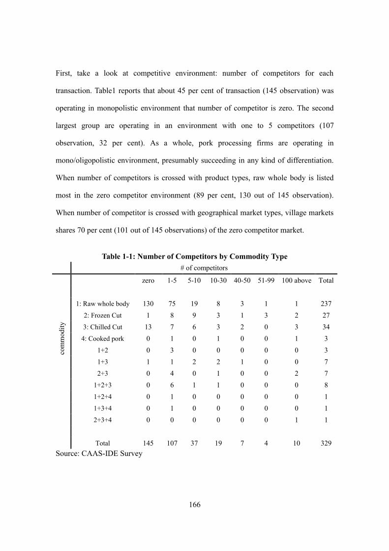
First, take a look at competitive environment: number of competitors for each

transaction. Table1 reports that about 45 per cent of transaction (145 observation) was

operating in monopolistic environment that number of competitor is zero. The second

largest group are operating in an environment with one to 5 competitors (107

observation, 32 per cent). As a whole, pork processing firms are operating in

mono/oligopolistic environment, presumably succeeding in any kind of differentiation.

When number of competitors is crossed with product types, raw whole body is listed

most in the zero competitor environment (89 per cent, 130 out of 145 observation).

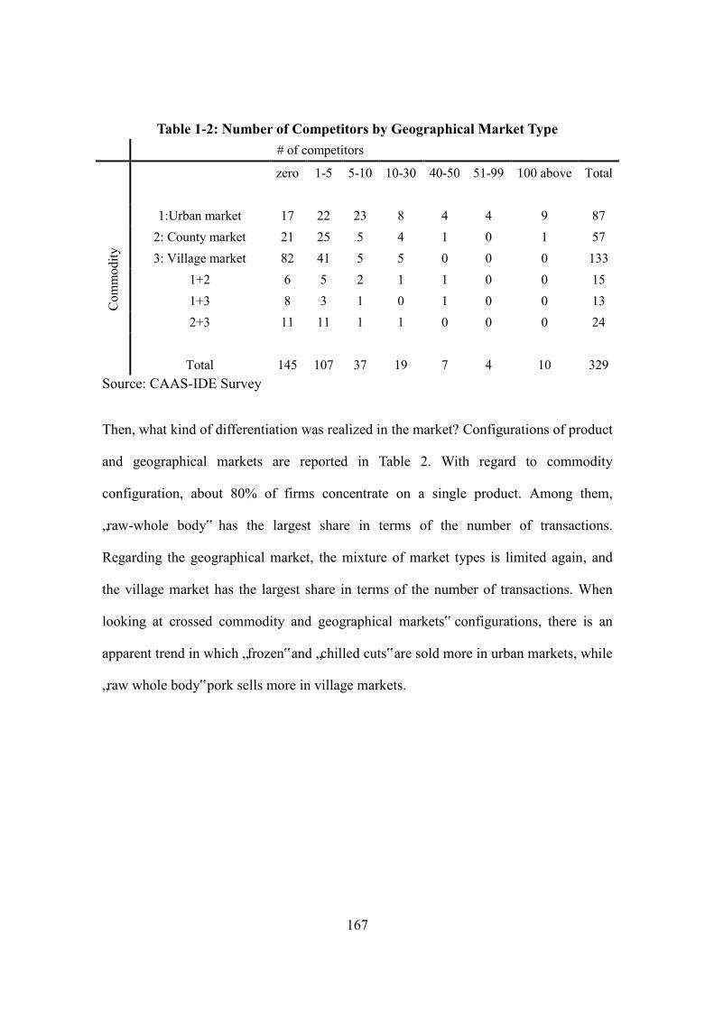
When number of competitor is crossed with geographical market types, village markets

shares 70 per cent (101 out of 145 observations) of the zero competitor market.

Table 1-1: Number of Competitors by Commodity Type

# of competitors

com

mod

ity

zero 1-5 5-10 10-30 40-50 51-99 100 above Total

1: Raw whole body 130 75 19 8 3 1 1 237 2: Frozen Cut 1 8 9 3 1 3 2 27 3: Chilled Cut 13 7 6 3 2 0 3 34

4: Cooked pork 0 1 0 1 0 0 1 3 1+2 0 3 0 0 0 0 0 3 1+3 1 1 2 2 1 0 0 7 2+3 0 4 0 1 0 0 2 7

1+2+3 0 6 1 1 0 0 0 8 1+2+4 0 1 0 0 0 0 0 1

1+3+4 0 1 0 0 0 0 0 1 2+3+4 0 0 0 0 0 0 1 1 Total 145 107 37 19 7 4 10 329

Source: CAAS-IDE Survey

167

Table 1-2: Number of Competitors by Geographical Market Type # of competitors

zero 1-5 5-10 10-30 40-50 51-99 100 above Total

Com

mod

ity

1:Urban market 17 22 23 8 4 4 9 87

2: County market 21 25 5 4 1 0 1 57 3: Village market 82 41 5 5 0 0 0 133

1+2 6 5 2 1 1 0 0 15 1+3 8 3 1 0 1 0 0 13 2+3 11 11 1 1 0 0 0 24

Total 145 107 37 19 7 4 10 329


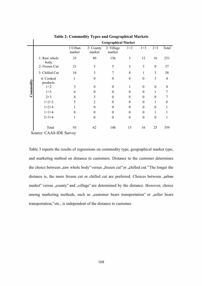
Then, what kind of differentiation was realized in the market? Configurations of product

and geographical markets are reported in Table 2. With regard to commodity

configuration, about 80% of firms concentrate on a single product. Among them,

„raw-whole body‟ has the largest share in terms of the number of transactions.

Regarding the geographical market, the mixture of market types is limited again, and

the village market has the largest share in terms of the number of transactions. When

looking at crossed commodity and geographical markets‟ configurations, there is an

apparent trend in which „frozen‟ and „chilled cuts‟ are sold more in urban markets, while

„raw whole body‟ pork sells more in village markets.

168

Table 2: Commodity Types and Geographical Markets Geographical Market

Com

mod

ity

1:Urban market

2: County market

3: Village market

1+2 1+3 2+3 Total

1: Raw whole body

35 49 136 3 12 16 251

2: Frozen Cut 21 5 5 3 3 0 37

3: Chilled Cut 16 3 7 8 1 3 38 4: Cooked products

1 0 0 0 0 3 4

1+2 3 0 0 1 0 0 4 1+3 6 0 0 0 0 1 7 2+3 4 3 0 0 0 0 7

1+2+3 5 2 0 0 0 1 8 1+2+4 1 0 0 0 0 0 1 1+3+4 0 0 0 0 0 1 1 2+3+4 1 0 0 0 0 0 1

Total 93 62 148 15 16 25 359


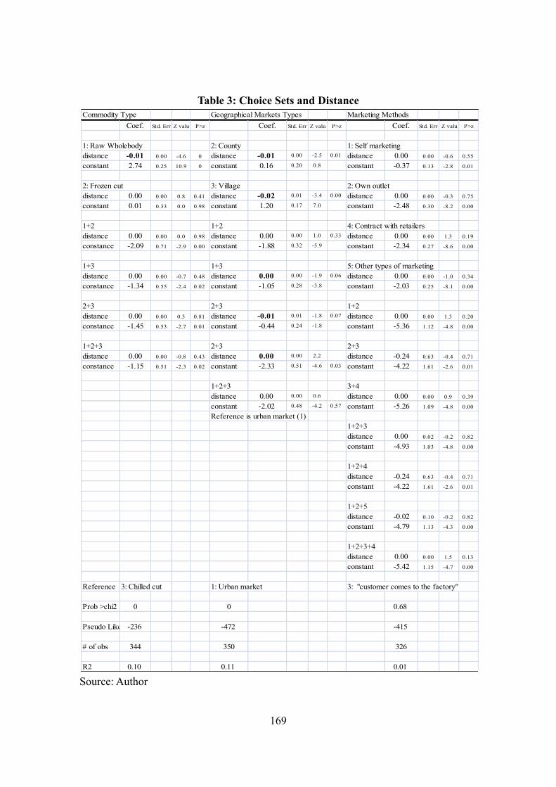
Table 3 reports the results of regressions on commodity type, geographical market type,

and marketing method on distance to customers. Distance to the customer determines

the choice between „raw whole body‟ versus „frozen cut‟ or „chilled cut.‟ The longer the

distance is, the more frozen cut or chilled cut are preferred. Choices between „urban

market‟ versus „county‟ and „village‟ are determined by the distance. However, choice

among marketing methods, such as „customer bears transportation‟ or „seller bears

transportation,‟ etc., is independent of the distance to customer.

169

Table 3: Choice Sets and Distance

Source: Author

Commodity Type Geographical Markets Types Marketing Methods Coef. Std. Err Z valu P>z Coef. Std. Err Z valu P>z Coef. Std. Err Z valu P>z

1: Raw Wholebody 2: County 1: Self marketingdistance -0.01 0.00 -4.6 0 distance -0.01 0.00 -2.5 0.01 distance 0.00 0.00 -0.6 0.55

constant 2.74 0.25 10.9 0 constant 0.16 0.20 0.8 constant -0.37 0.13 -2.8 0.01

2: Frozen cut 3: Village 2: Own outletdistance 0.00 0.00 0.8 0.41 distance -0.02 0.01 -3.4 0.00 distance 0.00 0.00 -0.3 0.75

constant 0.01 0.33 0.0 0.98 constant 1.20 0.17 7.0 constant -2.48 0.30 -8.2 0.00

1+2 1+2 4: Contract with retailersdistance 0.00 0.00 0.0 0.98 distance 0.00 0.00 1.0 0.33 distance 0.00 0.00 1.3 0.19

constance -2.09 0.71 -2.9 0.00 constant -1.88 0.32 -5.9 constant -2.34 0.27 -8.6 0.00

1+3 1+3 5: Other types of marketingdistance 0.00 0.00 -0.7 0.48 distance 0.00 0.00 -1.9 0.06 distance 0.00 0.00 -1.0 0.34


2+3 2+3 1+2distance 0.00 0.00 0.3 0.81 distance -0.01 0.01 -1.8 0.07 distance 0.00 0.00 1.3 0.20


1+2+3 2+3 2+3distance 0.00 0.00 -0.8 0.43 distance 0.00 0.00 2.2 distance -0.24 0.63 -0.4 0.71

constance -1.15 0.51 -2.3 0.02 constant -2.33 0.51 -4.6 0.03 constant -4.22 1.61 -2.6 0.01

1+2+3 3+4distance 0.00 0.00 0.6 distance 0.00 0.00 0.9 0.39

constant -2.02 0.48 -4.2 0.57 constant -5.26 1.09 -4.8 0.00

Reference is urban market (1)1+2+3distance 0.00 0.02 -0.2 0.82

constant -4.93 1.03 -4.8 0.00

1+2+4distance -0.24 0.63 -0.4 0.71

constant -4.22 1.61 -2.6 0.01

1+2+5distance -0.02 0.10 -0.2 0.82

constant -4.79 1.13 -4.3 0.00

1+2+3+4distance 0.00 0.00 1.5 0.13

constant -5.42 1.15 -4.7 0.00

Reference 3: Chilled cut 1: Urban market 3: "customer comes to the factory"

Prob >chi2 0 0 0.68

Pseudo Likelihood-236 -472 -415

# of obs 344 350 326

R2 0.10 0.11 0.01

170

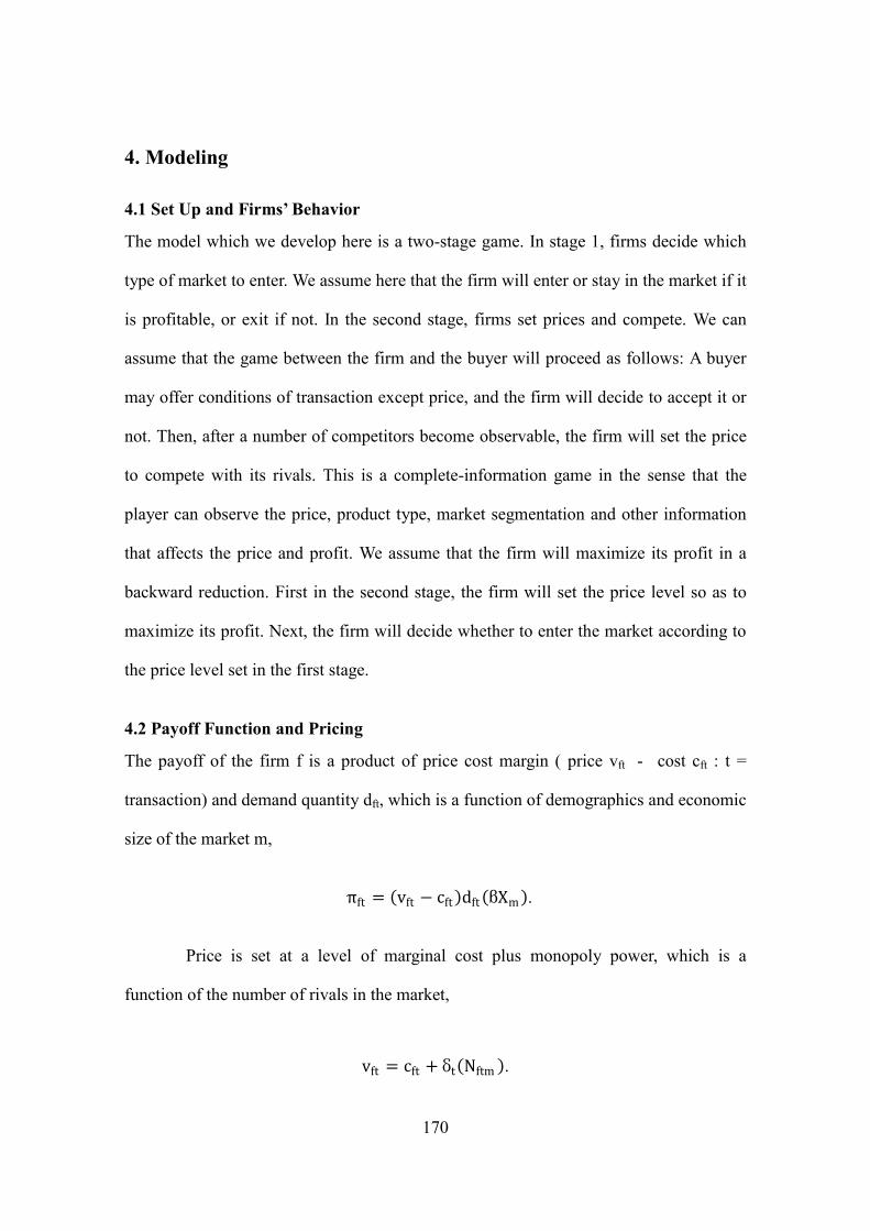
4. Modeling 4.1 Set Up and Firms’ Behavior

The model which we develop here is a two-stage game. In stage 1, firms decide which

type of market to enter. We assume here that the firm will enter or stay in the market if it

is profitable, or exit if not. In the second stage, firms set prices and compete. We can

assume that the game between the firm and the buyer will proceed as follows: A buyer

may offer conditions of transaction except price, and the firm will decide to accept it or

not. Then, after a number of competitors become observable, the firm will set the price

to compete with its rivals. This is a complete-information game in the sense that the

player can observe the price, product type, market segmentation and other information

that affects the price and profit. We assume that the firm will maximize its profit in a

backward reduction. First in the second stage, the firm will set the price level so as to

maximize its profit. Next, the firm will decide whether to enter the market according to

the price level set in the first stage.

4.2 Payoff Function and Pricing

The payoff of the firm f is a product of price cost margin ( price vft - cost cft : t =

transaction) and demand quantity dft, which is a function of demographics and economic

size of the market m,

πft = vft − cft dft βXm .

Price is set at a level of marginal cost plus monopoly power, which is a

function of the number of rivals in the market,

vft = cft + δt Nftm .

171

Marginal cost cft consists of the price of the pig pf, transportation cost tft

and cost to quality maintenance qft,

cft = pf + tft + qft .

The firm will set the price vft as high as possible so as to maximize its profit,

and thus the optimal price will be the marginal cost plus monopoly power. Firm-specific

factor and market specific factor remained unobservable to researcher.

vft∗ = cft + δt Nftm + σf + ωm + εftm (1).

Under this pricing strategy, optimal profit would be the product of monopoly

power, demographics and economic size of the market,

πft

∗ = δt Nftm + σf + ωm + εftm dft βXm (2).

Purpose of firm in differentiating their product is to maximize their monopoly

power, which brings profit maximization. Here the equilibrium is unique. In this

chapter, we will try to quantify monopoly power from two differentiation strategies, that

is, sizes of coefficients of product differentiation δp and that of geographical

differentiation δg , and compare which is more profitable for the firm.

4.3 Estimation

The final goal of estimation here is to obtain unbiased estimates of monopoly power

coefficients δp and δg in the price function (1). In this chapter, we will take a

Heckman two-step approach following Mazzeo (2002).

4.3.1 Correction of Sample Selection Bias due to Differentiation

Econometric problem here is that unobservable term εftm may be correlated with

172

observables, and in particular, coefficients of „number of competitors‟ δt , could be

biased. The source of this bias is a fact that the number of rivals and the competition

environment are endogenously determined with firm‟s differentiation strategy. If the

firm decides to operate in the product/geographical market t, the firm will set price vft.

Otherwise, we cannot observe price. This means that price vft is observable only in an

area larger than any critical point z. When applying this to the truncated sample, it is

known that we can obtain an unbiased estimator by explicitly introducing a selection

mechanism.

Expected value of price with a truncated sample conditional on observables x

(= cft + δt Nftm + σf + ωm ) can be obtained as follows:

E vft |x = E vft |x, vft > 𝑧 ･P vft > 𝑧|𝑥 + 0･P(vft = z|x).

The conditional probability that price vft whose variance is σ is larger than any critical

value z can be written as follows:

P vft |vft > 𝑧 = P εftm > 𝑧 − 𝑥𝛽 x = P εftm

σ>

z−xβ)

σ = Φ(

z−xβ

σ),

If any critical value z follows normal distribution with mean zero and variance 1, the

expected value of some variable y with a condition that y is larger than critical value z is

as follows,

E y|y > 𝑧 =� z

1−Φ z if z ∼ Normal(0,1).

Here, the conditional expected value of unobservable εftm becomes;

E εftm |εftm > 𝑧 − xβ = σE εftm

σ|εftm

σ>

z−xβ

σ = σ

ϕ{(z−xβ)/σ}

1−Φ z−xβ σ ,

Then, the expected value of price becomes the sum of observable xβ and times of

173

inverse Mills ratio.

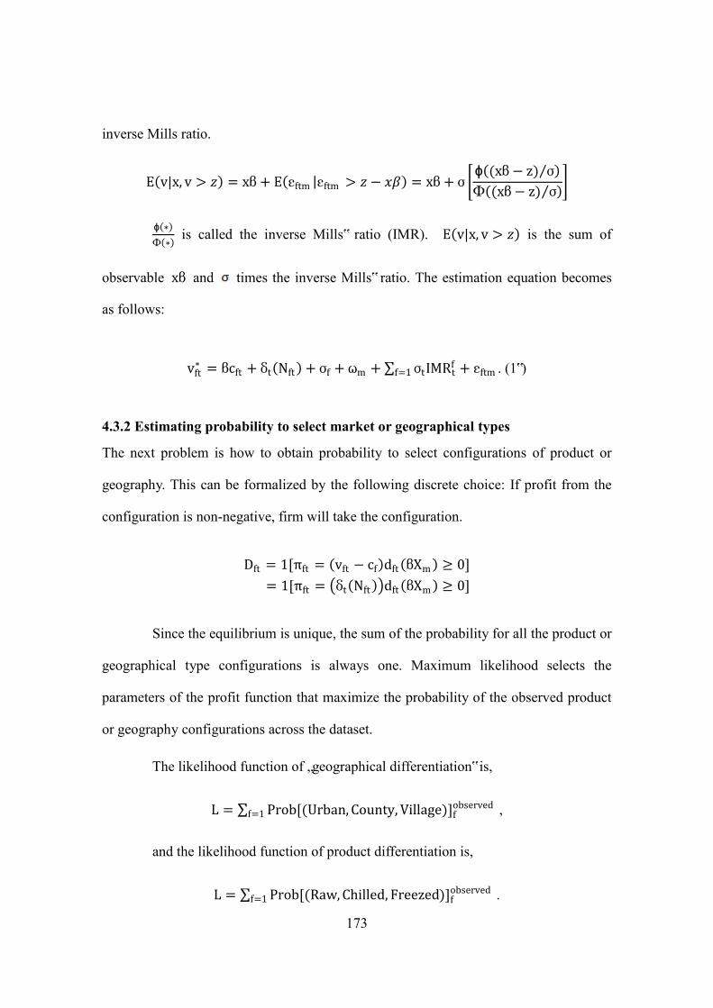
E v|x, v > 𝑧 = xβ + E εftm εftm > 𝑧 − 𝑥𝛽 = xβ + σ ϕ (xβ− z) σ

Φ (xβ− z) σ

ϕ ∗

Φ ∗ is called the inverse Mills‟ ratio (IMR). E v|x, v > 𝑧 is the sum of

observable xβ and times the inverse Mills‟ ratio. The estimation equation becomes

as follows:

vft∗ = βcft + δt Nft + σf + ωm + σtIMRt

ff=1 + εftm . (1‟)

4.3.2 Estimating probability to select market or geographical types

The next problem is how to obtain probability to select configurations of product or

geography. This can be formalized by the following discrete choice: If profit from the

configuration is non-negative, firm will take the configuration.

Dft = 1[πft = vft − cf dft βXm ≥ 0]

= 1[πft = δt Nft dft βXm ≥ 0]

Since the equilibrium is unique, the sum of the probability for all the product or

geographical type configurations is always one. Maximum likelihood selects the

parameters of the profit function that maximize the probability of the observed product

or geography configurations across the dataset.

The likelihood function of „geographical differentiation‟ is,

L = Prob[(Urban, County, Village)]fobserved

f=1 ,

and the likelihood function of product differentiation is,

L = Prob[(Raw, Chilled, Freezed)]fobserved

f=1 .

174

To estimate the likelihood function above, we use a maximum simulated likelihood

(MSL) approach. As our problems entail more than two choices, ordinary probit cannot

be used. Endogeneity correction method of truncated sample requires to the

unobservable follows normal distribution, not i.i.d. extreme values, so we cannot use

logit. Multinomial probit with simulation can compute the probability.3

4.4 Results

Tables 4 and 5 report the estimates of probability for select product/geographical

configurations.

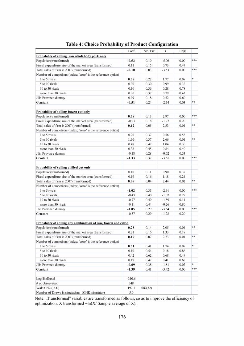
Product-choice-probability estimates reveal the following relationship: Estimated

parameters indicate the relative effects on profit and choice decision of differentiated

market conditions. Firstly, relative values of constants indicate that any single product is

preferred to a combination of raw whole body, frozen cut and chilled cut (constant of

combination = -1.39 versus constant of raw -.51, frozen -1.33 and -.37 chilled) if all

other observed variables are equal. Among choices in a single product, raw whole body

is preferred in a markets that population is smaller (the coefficient of population is -.53) ,

and is in oligopolistic (the coefficient of dummy 1 to 5 rivals is .38) and is preferred by

smaller firms (coefficient of sales = -0.1). Chilled cut is the opposite; it is preferred in

monopolistic markets (coefficient of dummy of 1 to 5 rivals is -1.02, which is

significant and the smallest) and is preferred by the larger firm (the coefficient of sales

= .09). Frozen cut is chosen in more competitive environment (coefficient of 5 to 10

3 Regarding details of multinomial probit, maximum simulated likelihood (MSL), method of simulated moment (MSM) see Stern (2000) and Train (2002). Simulation is used in these estimation methods so as to obtain a dimensional integral part of joint distribution among multi options that cannot be analytically solved.

175

rivals is 1, which is significant and the largest among choices), other conditions are

valued in between those of raw whole body and chilled cut.

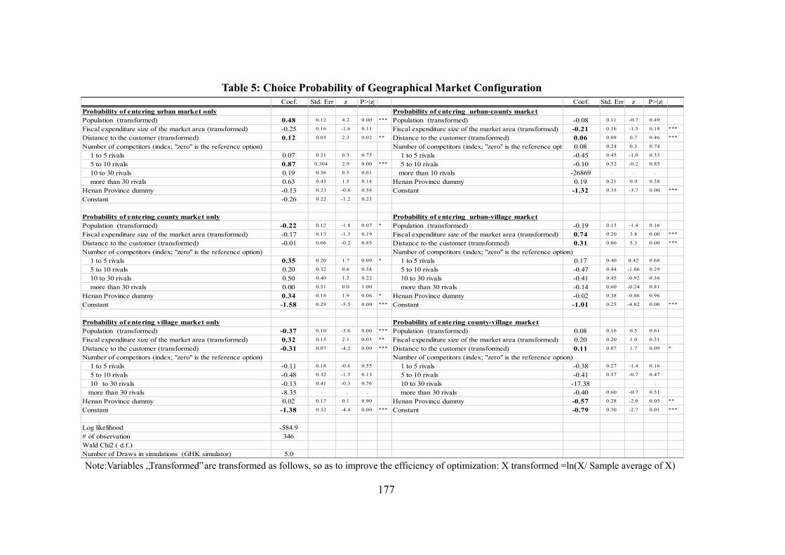
The results of geographical market choice estimates are somewhat complicated.

The dataset contains six choices of configuration of geographical market choice. The

constants of the six choices do not show systematic results. Only the constant of urban

market is not statistically significant, and the other coefficients of choice are more or

less at the same level. Coefficients for distance to the customers indicate that if the firm

can accept longer distances, the firm chooses only the urban market or an urban-county

or urban-village combinations. In contrast, a firm that cannot accept a longer distance to

the customer prefers to supply at only the village market.

176

Table 4: Choice Probability of Product Configuration

Note: „Transformed‟ variables are transformed as follows, so as to improve the efficiency of optimization: X transformed =ln(X/ Sample average of X).

Coef. Std. Err z P>|z|Probability of selling raw wholebody pork onlyPopulation(transformed) -0.53 0.10 -5.06 0.00 ***Fiscal expenditure size of the market area (transformed) 0.11 0.15 0.73 0.47Total sales of firm in 2007 (transformed) -0.10 0.03 -3.53 0.00 ***Number of competitors (index; "zero" is the reference option) 1 to 5 rivals 0.38 0.22 1.77 0.08 * 5 to 10 rivals 0.30 0.30 0.99 0.32 10 to 30 rivals 0.10 0.36 0.28 0.78 more than 30 rivals 0.30 0.37 0.79 0.43Jilin Province dummy 0.09 0.18 0.52 0.60Constant -0.51 0.24 -2.14 0.03 **

Probability of selling frozen cut onlyPopulation(transformed) 0.38 0.13 2.97 0.00 ***Fiscal expenditure size of the market area (transformed) -0.23 0.18 -1.27 0.20Total sales of firm in 2007 (transformed) 0.12 0.05 2.53 0.01 **Number of competitors (index; "zero" is the reference option) 1 to 5 rivals 0.20 0.37 0.56 0.58 5 to 10 rivals 1.00 0.37 2.66 0.01 ** 10 to 30 rivals 0.49 0.47 1.04 0.30 more than 30 rivals 0.38 0.45 0.84 0.40Jilin Province dummy -0.18 0.28 -0.62 0.53Constant -1.33 0.37 -3.61 0.00 ***

Probability of selling chilled cut onlyPopulation(transformed) 0.10 0.11 0.90 0.37Fiscal expenditure size of the market area (transformed) 0.19 0.16 1.18 0.24Total sales of firm in 2007 (transformed) 0.09 0.04 2.44 0.02 **Number of competitors (index; "zero" is the reference option) 1 to 5 rivals -1.02 0.35 -2.91 0.00 *** 5 to 10 rivals -0.43 0.40 -1.07 0.29 10 to 30 rivals -0.77 0.49 -1.59 0.11 more than 30 rivals -0.11 0.44 -0.26 0.80Jilin Province dummy -1.05 0.29 -3.64 0.00 ***Constant -0.37 0.29 -1.28 0.20

Probability of selling any combination of raw, frozen and cilledPopulation(transformed) 0.28 0.14 2.05 0.04 **Fiscal expenditure size of the market area (transformed) 0.21 0.16 1.33 0.18Total sales of firm in 2007 (transformed) 0.19 0.07 2.73 0.01 **Number of competitors (index; "zero" is the reference option) 1 to 5 rivals 0.71 0.41 1.74 0.08 * 5 to 10 rivals 0.10 0.54 0.18 0.86 10 to 30 rivals 0.42 0.62 0.68 0.49 more than 30 rivals 0.19 0.47 0.41 0.68Jilin Province dummy -0.69 0.38 -1.81 0.07 *Constant -1.39 0.41 -3.42 0.00 ***

Log likelihood -310.6# of observation 348Wald Chi2 ( d.f.) 197.1 chi2(32)Number of Draws in simulations (GHK simulator) 5.0

177

Table 5: Choice Probability of Geographical Market Configuration

Note:Variables „Transformed‟ are transformed as follows, so as to improve the efficiency of optimization: X transformed =ln(X/ Sample average of X)

Coef. Std. Err z P>|z| Coef. Std. Err z P>|z|Probability of entering urban market only Probability of entering urban-county marketPopulation (transformed) 0.48 0.12 4.2 0.00 *** Population (transformed) -0.08 0.11 -0.7 0.49

Fiscal expenditure size of the market area (transformed) -0.25 0.16 -1.6 0.11 Fiscal expenditure size of the market area (transformed) -0.21 0.16 -1.3 0.18 ***

Distance to the customer (transformed) 0.12 0.05 2.3 0.02 ** Distance to the customer (transformed) 0.06 0.08 0.7 0.46 ***

Number of competitors (index; "zero" is the reference option) Number of competitors (index; "zero" is the reference option) 0.08 0.24 0.3 0.74

1 to 5 rivals 0.07 0.21 0.3 0.75 1 to 5 rivals -0.45 0.45 -1.0 0.33

5 to 10 rivals 0.87 0.304 2.9 0.00 *** 5 to 10 rivals -0.10 0.52 -0.2 0.85

10 to 30 rivals 0.19 0.36 0.5 0.61 more than 10 rivals -26869 . . .

more than 30 rivals 0.63 0.43 1.5 0.14 Henan Province dummy 0.19 0.21 0.9 0.38

Henan Province dummy -0.13 0.23 -0.6 0.58 Constant -1.32 0.35 -3.7 0.00 ***

Constant -0.26 0.22 -1.2 0.23

Probability of entering county market only Probability of entering urban-village marketPopulation (transformed) -0.22 0.12 -1.8 0.07 * Population (transformed) -0.19 0.13 -1.4 0.16

Fiscal expenditure size of the market area (transformed) -0.17 0.13 -1.3 0.19 Fiscal expenditure size of the market area (transformed) 0.74 0.20 3.8 0.00 ***

Distance to the customer (transformed) -0.01 0.06 -0.2 0.85 Distance to the customer (transformed) 0.31 0.06 5.3 0.00 ***

Number of competitors (index; "zero" is the reference option) Number of competitors (index; "zero" is the reference option) 1 to 5 rivals 0.35 0.20 1.7 0.09 * 1 to 5 rivals 0.17 0.40 0.42 0.68



more than 30 rivals 0.00 0.51 0.0 1.00 more than 30 rivals -0.14 0.60 -0.24 0.81

Henan Province dummy 0.34 0.18 1.9 0.06 * Henan Province dummy -0.02 0.38 -0.06 0.96

Constant -1.58 0.29 -5.5 0.00 *** Constant -1.01 0.25 -4.02 0.00 ***

Probability of entering village market only Probability of entering county-village marketPopulation (transformed) -0.37 0.10 -3.6 0.00 *** Population (transformed) 0.08 0.16 0.5 0.61

Fiscal expenditure size of the market area (transformed) 0.32 0.15 2.1 0.03 ** Fiscal expenditure size of the market area (transformed) 0.20 0.20 1.0 0.31

Distance to the customer (transformed) -0.31 0.07 -4.2 0.00 *** Distance to the customer (transformed) 0.11 0.07 1.7 0.09 *

Number of competitors (index; "zero" is the reference option) Number of competitors (index; "zero" is the reference option) 1 to 5 rivals -0.11 0.18 -0.6 0.55 1 to 5 rivals -0.38 0.27 -1.4 0.16

5 to 10 rivals -0.48 0.32 -1.5 0.13 5 to 10 rivals -0.41 0.57 -0.7 0.47

10　to 30 rivals -0.13 0.41 -0.3 0.76 10 to 30 rivals -17.38 . . .

more than 30 rivals -8.35 . . . more than 30 rivals -0.40 0.60 -0.7 0.51

Henan Province dummy 0.02 0.17 0.1 0.90 Henan Province dummy -0.57 0.28 -2.0 0.05 **

Constant -1.38 0.32 -4.4 0.00 *** Constant -0.79 0.30 -2.7 0.01 ***

Log likelihood -584.9# of observation 346Wald Chi2 ( d.f.)Number of Draws in simulations (GHK simulator) 5.0

178

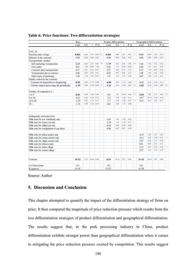
Table 6 reports the results of price regressions. What we focus on in this chapter is the

coefficients of number of rivals δt . The first column indicates the result of the price

regression (1‟) without correction of endogeneity. The second indicates the result of the

endogeneity correction by inserting the inverse Mills‟ ratio from product configuration

choice estimation. Coefficients of the number of rivals δp becomes larger than

regression without endogeneity correction for more than 5 competitors, but significant

only for the case with more than 30 competitors. The coefficients show how much the

price would increase/decrease compared to the zero-competitor environment. The

magnitude of impact on price reduction is for the group with more than 30 competitors,

2.1 RMB. This implies if product differentiation strategy taken, price is less elastic till

the competitors becomes as large as 30. What is interesting is if the customer will do

inspection of products, selling price is significantly reduced.

The third column reports the impact of geographical differentiation. The

coefficients of the number of rivals δg are significant and negative for the group with 1

to 5 competitors. Its magnitude is larger than in the case of product differentiation. With

the appearance of competitors numbering 1 to 5, the selling price is reduced by 4.2

RMB, which is the twice of the amount in the case of product differentiation. This

suggests that geographical differentiation can mitigate price reduction pressure less than

product differentiation.

Coefficients of the inverse Mills‟ ratio term are not strongly significant for both

the product-differentiated and the geographical-differentiated market. Coefficients of

the terms for frozen cut only are weakly significant and negative. This suggests that

there are unobserved factors which affect both observed price and product choice

179

probability in the opposite way. For example, if some factor encourages the choice to

sell only raw whole body, this will exert pressure on price.

There are some interesting results in relation to spatial economy. First, distance

to the customer has no power to explain price level. This is consistent for all the

estimation here. Secondly, a certain type of marketing and transportation method

matters price. Our data contains information on the transporting-marketing method: (1)

it is the seller firm that does marketing to the customer and transports the goods at the

seller‟s cost, (2) firms set up their own marketing outlets, (3) it is the customer who

goes to the firm and bears the transport cost, (4) it is the contracted distributor who does

the transportation and (5) others. Among these, „(1) the seller firm will bear the

marketing and transportation cost‟ is significant and positive. This means that if the

seller firm bears the transportation cost, then the selling price can be raised. However, if

the buyer bears the marketing and transportation cost, then the selling price is not

affected. Thus, there is asymmetry in the cost-bearing of transportation.

180

Table 6: Price functions: Two differentiation strategies

Source: Author 5. Discussion and Conclusion

This chapter attempted to quantify the impact of the differentiation strategy of firms on

price. It then compared the magnitude of price reduction pressure which results from the

two differentiation strategies of product differentiation and geographical differentiation.

The results suggest that, in the pork processing industry in China, product

differentiation exhibits stronger power than geographical differentiation when it comes

to mitigating the price reduction pressure exerted by competition. This results suggest

Base Product differentiation Geographical DifferentiationCoef. S.E. t P>|t| Coef. S.E. t P>|t| Coef. S.E. t P>|t|

Cost : βPurchase price of pigs 0.001 0.00 2.13 0.03 ** 0.001 0.00 1.81 0.07 * 0.001 0.001 1.58 0.12

Distance to the customer 0.00 0.00 0.60 0.55 0.00 0.00 0.48 0.63 0.00 0.00 -0.49 0.63

Transportation method Self marketing- transporation 2.13 0.83 2.57 0.01 ** 1.79 0.85 2.09 0.04 ** 1.66 1.36 1.23 0.22

Own outlet 0.01 1.09 0.00 1.00 0.23 1.15 0.20 0.84 0.20 1.61 0.13 0.90

Customer does transportation 0.51 0.81 0.63 0.53 0.27 0.82 0.33 0.75 0.12 1.30 0.09 0.93

Transporation due to contract 0.86 0.95 0.90 0.37 0.95 0.97 0.98 0.33 1.48 1.49 1.00 0.32

Other types of marketing 1.90 1.34 1.42 0.16 1.71 1.32 1.29 0.20 2.03 1.62 1.25 0.21

Quality control by the customer Customer do inspection on slaughtering -0.85 0.49 -1.75 0.08 * -0.88 0.51 -1.72 0.09 * -0.85 0.54 -1.58 0.12

Custmer inspect processing site periodically -1.19 0.50 -2.39 0.02 ** -1.21 0.54 -2.24 0.03 ** -1.02 0.54 -1.89 0.06 **

Number of competitors: δ1 to 5 -0.81 0.44 -1.86 0.06 * -0.6 1.51 -0.42 0.68 ** -4.84 2.82 -1.71 0.09 **

5 to 10 -0.21 0.64 -0.33 0.74 -2.2 1.49 -1.50 0.14 -14.7 10.19 -1.44 0.15

10 to 30 -1.25 0.92 -1.37 0.17 -1.7 1.39 -1.20 0.23 ** 72.9 53.0 1.38 0.17

30 - -1.18 0.90 -1.32 0.19 -2.1 1.20 -1.77 0.08

Endogeneity correction termMills ratio for raw wholebody only -2.01 1.68 -1.20 0.23

Mills ratio for frozen cut only -2.39 1.53 -1.56 0.12

Mills ratio for chilled cut only -0.42 0.96 -0.44 0.66

Mills ratio for configulation of any three 0.90 0.97 0.92 0.36

Mills ratio for urban market only -4.33 3.42 -1.27 0.21

Mills ratio for county market only -25.1 16.8 -1.49 0.14 *

Mills ratio for village market only 3.07 2.58 1.19 0.24

Mills ratio for urban-county 0.91 0.88 1.03 0.31

Mills ratio for urban-village -5.11 3.58 -1.43 0.16 *

Mills ratio for county-village 22.5 16.6 1.36 0.18

Constant 18.32 1.23 14.83 0.00 42.0 18.12 2.32 0.02 31.42 10.52 2.99 0.00

# of observation 313 313 313R-squared 0.118 0.137 0.129

181

that this difference may encourage firms to invest more in facilities that upgrading

product quality rather than securing geographical monopoly. However, the reality is

opposite. Most of our data set firms stay in geographical monopolistic positions thanks

to some power. The results reject that the power that secures geographical monopoly is

not distance to the customer or transportation cost. The results support that small

fragmented market may have inhibited spreading of high-quality pork production.

Development of the empirical method to differentiated markets or markets with

strategic interaction allows us to identify the location choice of the firms and to quantify

the impact of this choice on firms‟ profit. Henceforth, the combination of the techniques

of empirical industrial organization and spatial economy has the potential to produce

further valuable research findings.

Reference

Simon P. Anderson, André De Palma, Jacques-François Thisse(1992), Discrete Choice Theory

of Product Differentiation,” MIT Press Berry, Steven T.(1992) “Estimation of a Model of Entry in the Airline Industry” Econometrica,

Vol. 60, No. 4 (Jul., 1992), pp. 889-917 -- (1994) “Estimating Discrete-Choice Models of Product Differentiation “The RAND Journal

of Economics, Vol. 25, No. 2 (Summer, 1994), pp. 242-262 Berry, S. T., J. Levinson, A. Pakes (1995) “Automobile Prices in Market Equilibrium,”

Econometrica, Vol. 63, pp.841-889. Davis, Peter(2006) “Spatial Competition in Retail Markets: Movie Theaters,” The RAND

Journal of Economics, Vol.37, No.4 (Winter, 2006), pp.964-982. Hotelling, Harold(1929), “Stability in Competition,” The Economic Journal, Vol. 39, No. 153

(Mar., 1929), pp. 41-57 Mazzeo, M.(2002a) “Product Choice and Oligopoly Market Structure,” The RAND Journal of

Economics, Vol.33, No.2, (Summer, 2002), pp.221-242. --(2002b) “Competitive Outcomes in Product-Differentiated Oligopoly,” The Review of

Economics and Statistics, Vol.84, No.4, (November, 2002), pp.716-728.

182

Nevo, Aviv(2001) “Measuring market Power in the Ready-to-Eat Cereal Industry,” Econometrica, Vol. 69, No.2 (March, 2001), pp.307-342.

Nishida, Mitsukuni(2008) “Estimating a Model of Strategic Store-Network Choice,” NET Institute, Working Paper #08-27.

Pinske, J., M.E. Slade, and C. Brett(2002) “Spatial Price Competition: A Semiparametric Approach,” Econometrica, Vol.70, No.3 (May, 2002), pp.1111-1153.

Reiss, P.C. and Frank A. Wolak(2007) “Structural Econometric Modeling: Rationales and Examples from Industrial Organization ” in Handbook of Econometrics, Volume 6A, Elsivier.

Seim, K(2006), “An Empirical Model of Firm Entry with Endogenous Product-Type Choices,”

The RAND Journal of Economics, Vol.37, No.3, (Summer, 2006), pp.619-640. Smith, H.(2004) “Supermarket Choice and Supermarket Competition in Market Equilibrium,”

Review of Economic Studies, Vol.71, No.1 (January, 2004) pp.147-165. Stern, Steven(2000) “Simulation-based inference in econometrics: motivation and methods” in

Roberto Mariano, Til Schuermann and Melvyn J. Weeks ed., Simulation-based Inference

in Econometrics-Methods and Applications-. Cambridge University Press. Tirole, Jean (1988), The Theory of Industrial Organization, MIT Press Train, Kenneth E.(2003), Discrete Choice Methods with Simulation. Cambridge University

Press. U.K. Jia, Panle(2008) “What Happens when Wal-mart Come to Town: An Empirical Analysis of the

Discount Retailing Industry,” Econometrica, Vol.76, No.6 (November, 2008)

chapter 5 product differentiation versus …...with differentiation, where price or product choice...

Documents