Chapter 5: Process Scheduling

Chapter 5: Process Scheduling

• Basic Concepts

• Scheduling Criteria

• Scheduling Algorithms

• Multiple-Processor Scheduling• Multiple-Processor Scheduling

• Thread Scheduling

• Operating Systems Examples

• Algorithm Evaluation

2009/11/2 2

5.1 Basic Concepts

• The idea of multiprogramming:

– Keep several processes in memory. Every time one process

has to wait, another process takes over the use of the CPU

• CPU-I/O burst cycle: Process execution consists of a

cycle of CPU execution and I/O wait (i.e., CPU burstcycle of CPU execution and I/O wait (i.e., CPU burst

and I/O burst).

– Generally, there is a large number of short CPU bursts, and a

small number of long CPU bursts.

– An I/O-bound program would typically has many very short

CPU bursts.

– A CPU-bound program might have a few long CPU bursts

2009/11/2 3

Alternating Sequence of CPU And I/O Bursts

2009/11/2 4

Histogram of CPU-burst Times

2009/11/2 5

CPU Scheduler

• Selects from among the processes in memory

that are ready to execute, and allocates the CPU

to one of them

• CPU scheduling decisions may take place when a

process:

1. Switches from running to waiting state

2. Switches from running to ready state

3. Switches from waiting to ready

4. Terminates

• Scheduling under 1 and 4 is nonpreemptive

• All other scheduling is preemptive

2009/11/2 6

Preemptive Issues

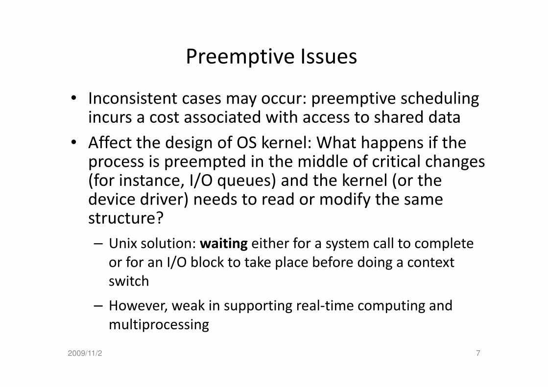
• Inconsistent cases may occur: preemptive scheduling incurs a cost associated with access to shared data

• Affect the design of OS kernel: What happens if the process is preempted in the middle of critical changes (for instance, I/O queues) and the kernel (or the device driver) needs to read or modify the same device driver) needs to read or modify the same structure?

– Unix solution: waiting either for a system call to complete

or for an I/O block to take place before doing a context

switch

– However, weak in supporting real-time computing and

multiprocessing

2009/11/2 7

Dispatcher

• Dispatcher module gives control of the CPU to the

process selected by the short-term scheduler; this

involves:

– switching context

– switching to user mode– switching to user mode

– jumping to the proper location in the user program to

restart that program

• Dispatch latency – time it takes for the dispatcher

to stop one process and start another running

2009/11/2 8

5.2 Scheduling Criteria

• CPU utilization – keep the CPU as busy as possible

• Throughput – # of processes that complete their

execution per time unit

• Turnaround time – amount of time to execute a

particular processparticular process

• Waiting time – amount of time a process has been

waiting in the ready queue

• Response time – amount of time it takes from

when a request was submitted until the first

response is produced, not output (for time-

sharing environment)

2009/11/2 9

Optimization Criteria

• Max CPU utilization

• Max throughput

• Min turnaround time

• Min waiting time •

• Min response time

2009/11/2 10

5.3 Scheduling Algorithms

• First-come, first-served (FCFS) scheduling

• Shortest-job-first (SJF) scheduling

• Priority scheduling

• Round-robin scheduling• Round-robin scheduling

• Multilevel queue scheduling

• Multilevel feedback queue scheduling

2009/11/2 11

First-Come, First-Served (FCFS) Scheduling

Process Burst Time

P1 24

P2 3

P3 3

• Suppose that the processes arrive in the order: P1 , P2 , P3

The Gantt Chart for the schedule is:The Gantt Chart for the schedule is:

• Waiting time for P1 = 0; P2 = 24; P3 = 27

• Average waiting time: (0 + 24 + 27)/3 = 17

P1 P2 P3

24 27 300

2009/11/2 12

FCFS Scheduling (Cont.)

• Suppose that the processes arrive in the order

P2 , P3 , P1

• The Gantt chart for the schedule is:

P1P3P2

• Waiting time for P1 = 6; P2 = 0; P3 = 3

• Average waiting time: (6 + 0 + 3)/3 = 3

• Much better than previous case

• Convoy effect short process behind long process

63 300

2009/11/2 13

Shortest-Job-First (SJR) Scheduling

• Associate with each process the length of its next

CPU burst. Use these lengths to schedule the

process with the shortest time

• Two schemes:

– nonpreemptive – once CPU given to the process it cannot

be preempted until completes its CPU burstbe preempted until completes its CPU burst

– preemptive – if a new process arrives with CPU burst

length less than remaining time of current executing

process, preempt. This scheme is know as the

Shortest-Remaining-Time-First (SRTF)

• SJF is optimal – gives minimum average waiting

time for a given set of processes

2009/11/2 14

Example of Non-Preemptive SJF

Process Arrival Time Burst Time

P1 0.0 7

P2 2.0 4

P3 4.0 1

P4 5.0 4

SJF (non-preemptive)• SJF (non-preemptive)

• Average waiting time = (0 + 6 + 3 + 7)/4 = 4

P1 P3 P2

73 160

P4

8 12

2009/11/2 15

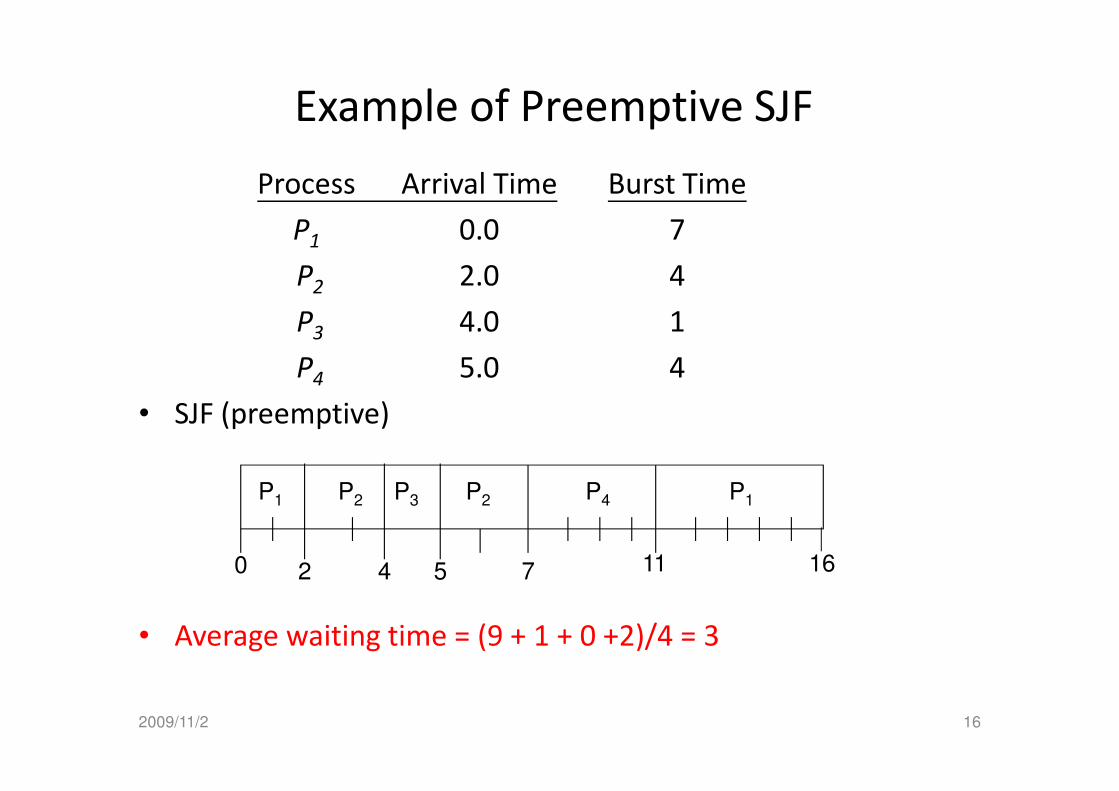
Example of Preemptive SJF

Process Arrival Time Burst Time

P1 0.0 7

P2 2.0 4

P3 4.0 1

P4 5.0 4

• SJF (preemptive)• SJF (preemptive)

• Average waiting time = (9 + 1 + 0 +2)/4 = 3

P1 P3P2

42 110

P4

5 7

P2 P1

16

2009/11/2 16

Determining Length of Next CPU Burst

• Frequently used in long-term scheduling

– A user is asked to estimate the job length. A lower value

means faster response. Too low a value will cause timeout.

• Approximate SJF: the next burst can be predicted as an exponential average of the measured length of previous CPU burstsprevious CPU bursts

nnnt τ)α1(ατ 1 −+=

+

... )2

1( )

2

1( )

2

1(

...α)α1(α)α1(α

2

3

1

2

2

2

1

+++=

+−+−+=

−−

−−

nnn

nnn

ttt

ttt

1/2

Commonly,

=α

history

new one

2009/11/2 17

Prediction of the Length of the Next CPU

Burst

2009/11/2 18

Examples of Exponential Averaging

• α =0

– τn+1 = τn

– Recent history does not count

• α =1

– τ = α t = t– τn+1 = α tn = tn

– Only the actual last CPU burst counts

• Since both α and (1 - α) are less than or equal to 1, each successive term has less weight than its predecessor

2009/11/2 19

Priority Scheduling

• A priority number (integer) is associated with each

process

• The CPU is allocated to the process with the

highest priority (smallest integer ≡ highest priority)

– Preemptive

– nonpreemptive– nonpreemptive

• SJF is a priority scheduling where priority is the

predicted next CPU burst time

• Problem: Starvation – low priority processes may

never execute

• Solution: Aging – as time progresses increase the

priority of the process2009/11/2 20

Process Burst Time Priority

P1 10 3

P2 1 1

P3 2 4

P4 1 5

P5 5 2

• An Example

P5 5 2

P5 P3

0 1 6 16 18 19

P4P2 P1

AWT = (6+0+16+18+1)/5=8.2

2009/11/2 21

Round Robin (RR)

• Each process gets a small unit of CPU time (time

quantum), usually 10-100 milliseconds. After this

time has elapsed, the process is preempted and

added to the end of the ready queue.

• If there are n processes in the ready queue and the • If there are n processes in the ready queue and the

time quantum is q, then each process gets 1/n of the

CPU time in chunks of at most q time units at once.

No process waits more than (n-1)q time units.

• Performance

– q large ⇒ FIFO

– q small ⇒ q must be large with respect to context switch,

otherwise overhead is too high2009/11/2 22

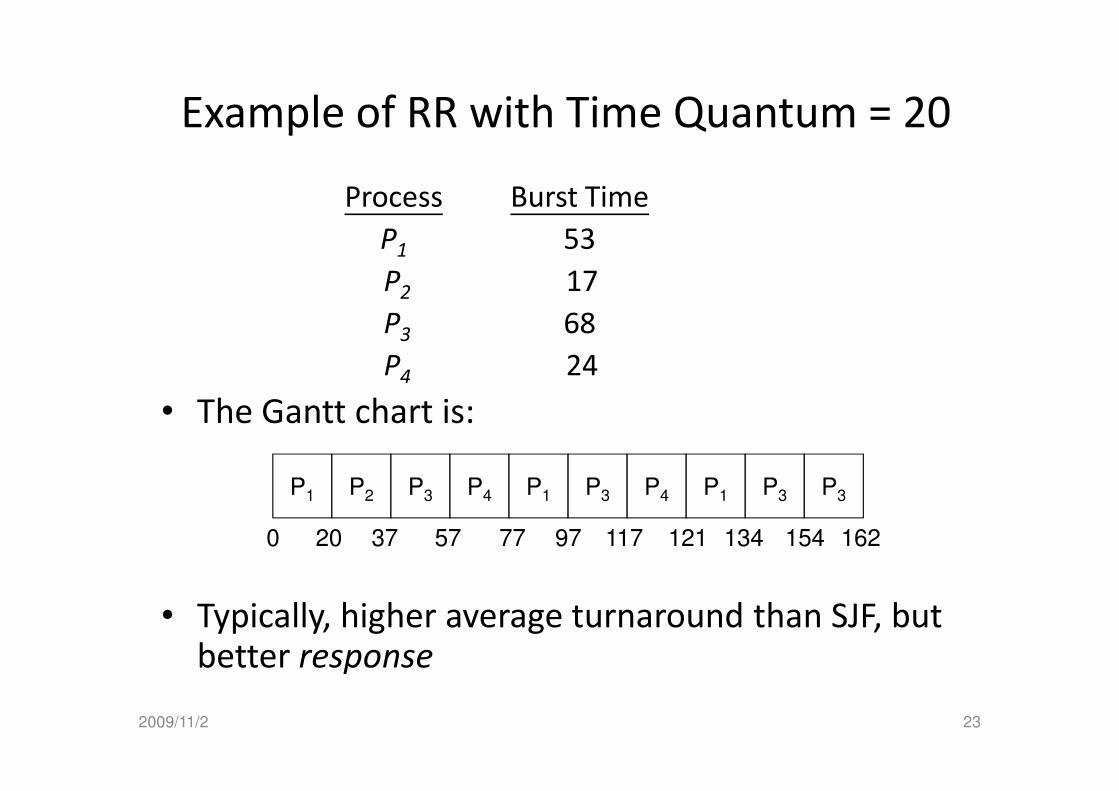
Example of RR with Time Quantum = 20

Process Burst Time

P1 53

P2 17

P3 68

P4 24

• The Gantt chart is: • The Gantt chart is:

• Typically, higher average turnaround than SJF, but better response

P1 P2 P3 P4 P1 P3 P4 P1 P3 P3

0 20 37 57 77 97 117 121 134 154 162

2009/11/2 23

Time Quantum and Context Switch Time

2009/11/2 24

Turnaround Time Varies With The Time

Quantum

q=1q=1p1p2p3p4p1p2p4p1p2p4p1p4p1p4p1p4p4

1 2 3 4 5 6 7 8 9 0 1 2 3 4 5 6 7

q=2

p1p2p3p4p1 p2 p4 p1 p4 p4

2 4 5 7 9 10 12 14 16 17

2009/11/2 25

Multilevel Queue

• Ready queue is partitioned into separate queues:foreground (interactive) and background (batch)

• Each queue has its own scheduling algorithm

– foreground – RR

– background – FCFS

• Scheduling must be done between the queues• Scheduling must be done between the queues

– Fixed priority scheduling; (i.e., serve all from foreground then from background). Possibility of starvation.

– Time slice: each queue gets a certain amount of CPU time which it can schedule amongst its processes; i.e., 80% to foreground in RR

– 20% to background in FCFS

2009/11/2 26

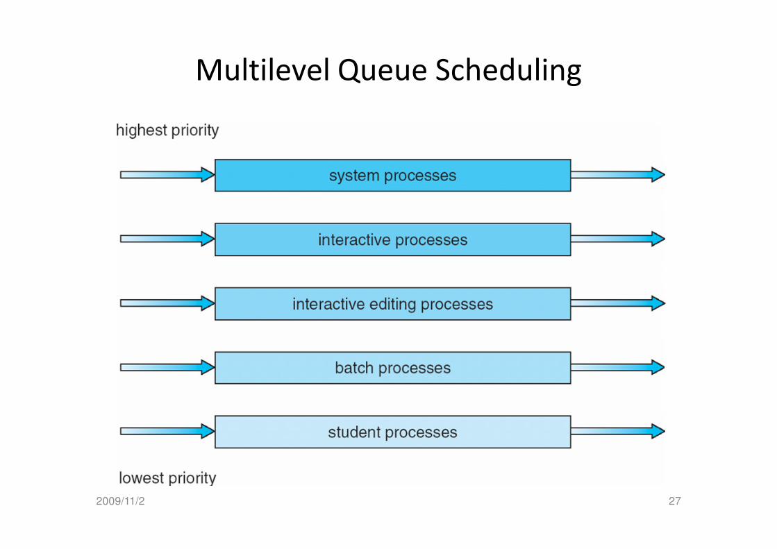
Multilevel Queue Scheduling

2009/11/2 27

Multilevel Feedback Queue

• A process can move between the various queues;

aging can be implemented this way

• Multilevel-feedback-queue scheduler defined by the

following parameters:

– number of queues– number of queues

– scheduling algorithms for each queue

– method used to determine when to upgrade a process

– method used to determine when to downgrade a process

– method used to determine which queue a process will

enter when that process needs service

2009/11/2 28

Example of Multilevel Feedback Queue

• Three queues:

– Q0 – RR with time quantum 8 milliseconds

– Q1 – RR time quantum 16 milliseconds

– Q2 – FCFS

• Scheduling• Scheduling

– A new job enters queue Q0 which is served FCFS. When it

gains CPU, job receives 8 milliseconds. If it does not finish

in 8 milliseconds, job is moved to queue Q1.

– At Q1 job is again served FCFS and receives 16 additional

milliseconds. If it still does not complete, it is preempted

and moved to queue Q2.

2009/11/2 29

Multilevel Feedback Queues

2009/11/2 30

5.4 Thread Scheduling

• Distinction between user-level and kernel-level threads

• Many-to-one and many-to-many models, thread library schedules user-level threads to run on LWP

Known as process-contention scope (PCS) since – Known as process-contention scope (PCS) since scheduling competition is within the process

• Kernel thread scheduled onto available CPU is system-contention scope (SCS) – competition among all threads in system

2009/11/2 31

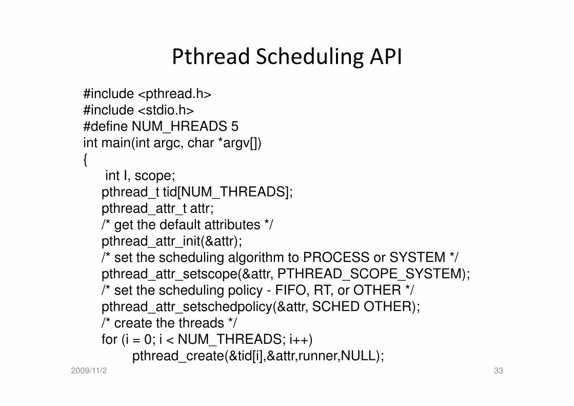
Pthread Scheduling

• API allows specifying either PCS or SCS

during thread creation

– PTHREAD_SCOPE_PROCESS schedules threads

using PCS schedulingusing PCS scheduling

– PTHREAD_SCOPE_SYSTEM schedules threads

using SCS scheduling.

2009/11/2 32

Pthread Scheduling API

#include <pthread.h>#include <stdio.h>#define NUM_HREADS 5int main(int argc, char *argv[]){

int I, scope;pthread_t tid[NUM_THREADS];pthread_attr_t attr;pthread_attr_t attr;/* get the default attributes */pthread_attr_init(&attr);/* set the scheduling algorithm to PROCESS or SYSTEM */pthread_attr_setscope(&attr, PTHREAD_SCOPE_SYSTEM);/* set the scheduling policy - FIFO, RT, or OTHER */pthread_attr_setschedpolicy(&attr, SCHED OTHER);/* create the threads */for (i = 0; i < NUM_THREADS; i++)

pthread_create(&tid[i],&attr,runner,NULL);2009/11/2 33

Pthread Scheduling API

/* now join on each thread */

for (i = 0; i < NUM_THREADS; i++)

pthread_join(tid[i], NULL);

}

/* Each thread will begin control in this function */

void *runner(void *param)void *runner(void *param)

{

printf("I am a thread\n");

pthread exit(0);

}

2009/11/2 34

5.5 Multiple-Processor Scheduling

• CPU scheduling more complex when multiple CPUs are available

• Homogeneous processors within a multiprocessor

• Asymmetric multiprocessing – only one processor accesses the system data structures, alleviating the need for data sharing

• Symmetric multiprocessing (SMP) – each processor is self-• Symmetric multiprocessing (SMP) – each processor is self-scheduling, all processes in common ready queue, or each has its own private queue of ready processes

• Processor affinity – process has affinity for processor on which it is currently running– soft affinity: OS has a policy of attempting to keep a process

running on the same processor but not guaranteeing that it will do so

– hard affinity: allowing a process to specify the desired processors

2009/11/2 35

NUMA and CPU Scheduling

2009/11/2 36

NUMA: Non-Uniform Memory Access

Load Balancing

• Attempts to keep the workload evenly distributed

across all processors

• Two general approaches can be implemented in

parallel :

– Push migration: a specific task periodically checks the load – Push migration: a specific task periodically checks the load

on each processor

– Pull migration: an idle processor pulls a waiting task from a

busy processor

• Contracts the benefits of processor affinity

– Processes are moved only if the imbalance exceeds a

certain threshold

2009/11/2 37

Multicore Processors

• Recent trend to place multiple processor cores

on same physical chip

• Faster and consume less power

• Multiple threads per core also growing• Multiple threads per core also growing

– Takes advantage of memory stall to make progress

on another thread while memory retrieve

happens

2009/11/2 38

Multithreaded Multicore System

2009/11/2 39

Memory stall

Multithreaded multicore system

5.6 Operating System Examples

• Solaris scheduling

• Windows XP scheduling

• Linux scheduling

2009/11/2 40

Solaris 2 Scheduling

2009/11/2 41

Solaris Scheduling

• Four classes of scheduling: real-time -> system ->

interactive -> time sharing.

• A process starts with one LWP and is able to create

new LWPs as needed. Each LWP inherits the

scheduling class and priority of the parent process. scheduling class and priority of the parent process.

Default : time sharing (multilevel feedback queuemultilevel feedback queue)

• Inverse relationship between priorities and time

slices: the high the priority, the smaller the time slice.

• Interactive processes typical have a higher priority;

CPU-bound processes have a lower priority.

2009/11/2 42

Solaris Scheduling

• Uses the system classsystem class to run kernel processes, such

as the scheduler and paging daemon. The system

class is reserved for kernel use onlykernel use only. User process

running in kernel mode are not in the system class.

• Threads in the real-time class are given the highest • Threads in the real-time class are given the highest

priority to run among all classes.

• There is a set of priorities within each class. However,

the scheduler converts the class-specific priorities

into global priorities. (round-robin queue)

2009/11/2 43

Solaris Dispatch Table (for interactive and

time-sharing threads)

2009/11/2 44

Solaris Scheduling

2009/11/2 45

Dispatch Table

• Priority: a higher number indicates a higher priority

• Time quantum: the lower priority has the higher

time quantum

• Time quantum expired: the new priority of a thread

that has used its entire time quantum without that has used its entire time quantum without

blocking. Such threads are considered CPU-intensive.

Lower priority of these thread

• Return from sleep: the priority of a thread that is

returning from sleeping (such as waiting for I/O). Its

priority is boosted to between 50 and 59.

2009/11/2 46

Windows XP Priorities

2009/11/2 47

Windows XP Scheduling

• Using a priority-based, preemptive scheduling

algorithm

• There are 32-level priority which are divided

into two classes

– The variable class contains priorities from 1 to 15– The variable class contains priorities from 1 to 15

– The real-time class contains threads from 16 to 31

• Within each of the priority classes is a relative

priority

• The priority of each thread is based on the

priority class it belongs to and its relative

priority within that class.2009/11/2 48

Linux Scheduling – preemptive & priority

• Version 2.5: support SMP, Load balancing & Processor affinity

• Time-sharing (100-140) and Real-time (0-99)

• Higher priority with longer time quanta

• Time-sharing

– Prioritized credit-based – process with most credits is scheduled next

– Credit subtracted when timer interrupt occurs

– When credit = 0, another process chosen– When credit = 0, another process chosen

– When all processes have credit = 0, recrediting occurs

• Based on factors including priority and history

• Real-time

– Soft real-time

– Posix.1b compliant – two classes

• FCFS and RR

• Highest priority process always runs first

2009/11/2 49

The Relationship Between Priorities and Time-

slice length

2009/11/2 50

List of Tasks Indexed According to

Priorities

2009/11/2 51

5.7 Algorithm Evaluation

• Criteria to select a CPU scheduling algorithm may include several measures, such as:

– Maximize CPU utilization under the constraint that the maximum response time is 1 second

– Maximize throughput such that turnaround time is (on average) linearly proportional to total execution timeaverage) linearly proportional to total execution time

• Evaluation methods ?

– deterministic modeling

– queuing models

– simulations

– implementation

2009/11/2 52

Deterministic Modeling

• Analytic evaluation

Input: a given algorithm and a system workload to

Output: performance of the algorithm for that workload

• Deterministic modeling (one type of analytic evaluation)

– Taking a particular predetermined workload and defining the performance of each algorithm for that workload.

2009/11/2 53

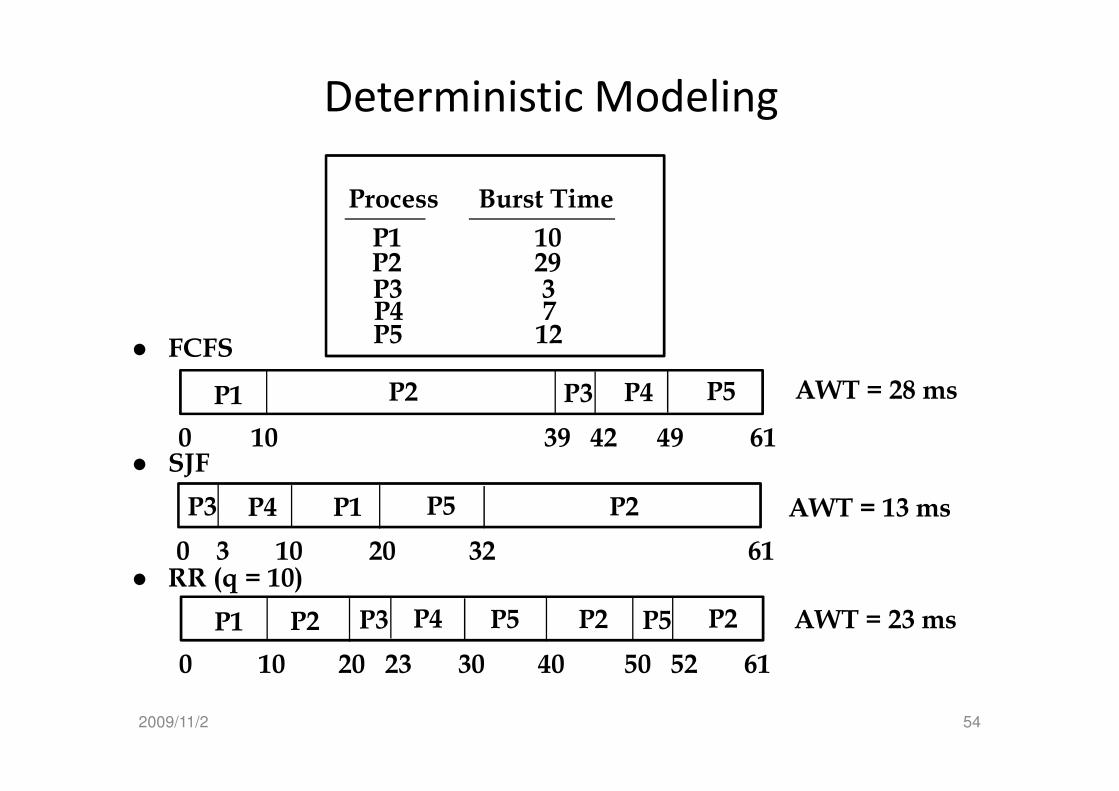
Deterministic Modeling

� FCFS

Process Burst Time

P1 10 P2 29P3 3P4 7

P5P3 P4P2P1

P5 12

AWT = 28 ms

� SJF

� RR (q = 10)

P5P3

0 10 39 42 49 61

P4P2P1

P5P3

0 3 10 20 32 61

P4 P2P1

P5P3

0 10 20 23 30 40 50 52 61

P4P2P1 P2 P2P5

AWT = 28 ms

AWT = 13 ms

AWT = 23 ms

2009/11/2 54

Deterministic Modeling

• A simple and fast method. It gives the exact numbers, allows the algorithms to be compared.

• It requires exact numbers of input, and its answers apply to only those cases. In general, deterministic modeling is too specific, and deterministic modeling is too specific, and requires too much exact knowledge, to be useful.

• Usage– Describing algorithm and providing examples

– A set of programs that may run over and over again and can measure the program’s processing requirement exactly

– Indicating the trends that can then be proved

2009/11/2 55

Queuing Models

• Queuing network analysis

– Using

• the distributiondistribution of service times (CPU and I/O bursts)

• the distributiondistribution of process arrival times

– The computer system is described as a network of servers. – The computer system is described as a network of servers.

Each server has a queue of waiting processes.

– Determining

• utilization, average queue length, average waiting time,

and so on

2009/11/2 56

Queuing Models

• Little's formula (for a stable system):

n = λ × W

n : average queue lengthn : average queue length

W: average waiting time

queue server

λλ : average arrival : average arrival

raterate

14 persons in queue =14 persons in queue =

7 arrives/per second 7 arrives/per second ××××××××

22 seconds waitingseconds waiting

• Queuing analysis can be useful in comparing scheduling algorithms, but it also has limitations.

• Queuing model is only an approximation of a real system. Thus, the result is questionable.

– The arrival and service distributions are often defined in unrealistic, but mathematically tractable, ways.

– Besides, independent assumptions may not be true.

W: average waiting time

2009/11/2 57

Simulations

• Simulations involve programming a model of the system. Software data structures represent the major components of the system.

• Simulations get a more accurate evaluation of scheduling algorithms.

– expensive (several hours of computer time).– expensive (several hours of computer time).

– large storage

– coding a simulator can be a major task

• Generating data to drive the simulator

– a random number generator.

–– trace tapestrace tapes: created by monitoring the real system, recording the sequence of actual events.

2009/11/2 58

Evaluation of CPU Schedulers by

Simulation

2009/11/2 59

Implementation

• Put data into a real system and see how it works.

• The only accurate way

– cost is too high– cost is too high

– environment will change (All methods have this problem!)

– e.g., To avoid moving to a lower priority queue, a user may output a meaningless character on the screen regularly to keep itself in the interactive queue.

2009/11/2 60

End of Chapter 5

Home WorkHome Work

• 5, 7, 13

• Due Nov. 12

2009/11/2 62