chapter 5 new concepts for managing urban pollution

Chapter 5New Concepts for Managing Urban Pollution

Lawrence A. Baker

5.1 Introduction

5.1.1 Chapter Goals

Most current pollution management in cities is based on treating pollution at theend-of-the pipe, after pollution is generated. This paradigm worked well for treatingmunicipal sewage and industrial effluents – point sources of pollutants. Pollutionfrom these sources has been greatly reduced since passage of the Clean Water Act in1972. However, the remaining pollution problem in post-industrial cities is mostlycaused by nonpoint sources – runoff from lawns, erosion from construction sites,gradual decomposition of automobiles (e.g., erosion of tire particles containing zincand brake pad linings with copper), and added road salt from de-icing operations.The next section of this chapter shows why the end-of-pipe paradigm cannot be theprimary approach for dealing with these types of pollution and why new approachesare needed.

If the traditional end-of-pipe paradigm doesn’t work, what will? I will argue thata new paradigm must be based on analysis of the movement of pollutants throughurban ecosystems, an approach sometimes called materials flow analysis (MFA).MFA can be used to identify where a potential pollutant enters an urban ecosystem,how it is transferred from one ecosystem compartment to another, and ultimately,it enters surface or groundwater to become an actual pollutant. As we will see,MFA can be used to guide the development of novel approaches for pollution man-agement: reducing inputs of potentially polluting materials to urban ecosystems,improving the efficiency by which they are utilized for their intended purposes, andrecycling them. MFA can also be used to develop strategies to mitigate legacy pol-

L.A. Baker (B)Minnesota Water Resources Center, University of Minnesota, and WaterThink, LLC, St. Paul,Minnesota, USAe-mail: [email protected]

L.A. Baker (ed.), The Water Environment of Cities,DOI 10.1007/978-0-387-84891-4 5, C© Springer Science+Business Media, LLC 2009

69

70 L.A. Baker

lution. The second goal of this chapter is to develop the basic concepts of MFA anddemonstrate its application in case studies.

The new paradigm for urban pollution management must also recognize therole of individuals and households in generating pollution – and in reducing it.In modern, post-industrial cities, much of the pollution is generated by the activitiesof individuals and households, and reducing pollution requires that people changetheir behaviors. Therefore, the third goal of this chapter is to examine several con-ceptual models that social scientists use to understand environmental behaviors andseveral case studies to illustrate how “soft” policy approaches can succeed in reduc-ing pollution or achieving other environmental goals.

Finally, the new paradigm for urban pollution management will make greater useof adaptive management. Adaptive management is the concept of using feedbackfrom the environment to managers (individuals; government agencies, etc.) to mod-ify ongoing management practices. Expanded use of adaptive management, madepossible by advances in sensor technology and by vast increases in our capacity toacquire, transmit, and store data, could lead to much greater use of adaptive man-agement for managing urban pollution. The final goal of this chapter is to examinethe application for adaptive management for managing urban pollution.

Several case studies – managing lawn runoff, reducing the legacy of urban leadpollution, and managing road salt – are developed to illustrate how these conceptscan be applied to problems of urban water management and pollution.

5.2 Limitations to End-of-Pipe Pollution Control

5.2.1 Success at Treating Point Sources of Pollution

The traditional focus of urban water pollution management in cities has been treat-ment of point sources of wastewater – mainly municipal sewage and industrialwastes. Modern wastewater treatment plants are essentially high-speed biogeochem-ical reactors where pollutants are degraded or transformed into manageable endproducts, such as sludge or harmless gases (Table 5.1). Physical and biological pro-cesses remove pollutants within a few hours in sewage treatment plants, whereasa similar level of pollutant conversion would take days to weeks in a river, duringwhich time pollutants would impact the river. Some pollutants are actually degradedby biological processes. For example, organic matter (measured as biological oxy-gen demand, or BOD) is converted to CO2 (Table 5.1). Many other pollutants donot actually disappear, but are “removed” only in the sense that they are transferredfrom the polluted water to sludge (biosolids) by sedimentation. The resulting sludgethen contains the pollutants.

Fifty years ago, many sewage treatment systems would have been some versionof sewage ponds, sometimes aerated. These were moderately effective at reducingthe BOD in sewage, but did little to remove nutrients (Table 5.1). Sewage lagoonsare still common in many small towns in rural areas of the United States and in

5 New Concepts for Managing Urban Pollution 71

Table 5.1 Treatment reactions, end products, and typical treatment efficiencies for several typesof municipal sewage treatment

Typical treatment efficiencies, as %of inflow concentrations

TypicalEnd Sewage secondary Advanced

Pollutant Reaction product ponds2 treatment3 treatment3

Biologicaloxygendemand(BOD)

Respiration CO2 50–95 95 95

Nitrogen Sedimentation,mineralization,nitrification-denitrification1

SludgeN2 gas

43–80 50 87

Phosphorus Concentration bymicrobes orchemical reactionwith alum

Sludge 50 51 85

Suspendedsolids

Sedimentation Sludge 85 95 95

Metals Chemicalprecipitation andsedimentation.

Sludge Variable Variable Variable

1Mineralization converts organic nitrogen to ammonium (NH4+); nitrification converts NH4

+ tonitrate (NO3

−); and denitrification converts nitrate to nitrogen gas (N2). All three processes aremediated by bacteria.2Values for lagoon systems are from Metcalf and Eddy (1991) and Reed (1995). Variability reflectswide variations in types of sewage pond (lagoon) designs.3Values for BOD, N and P removal are averages for secondary and advanced treatment systems inthe St. Paul-Minneapolis metropolitan region. Suspended solids removal is a “typical” value.

larger cities in lesser developed countries, but the majority of wastewater systemsin U.S. cities use at least “secondary” treatment, high tech systems that can removeup to 95% of organic matter. What was once called “advanced treatment” – addi-tional processes used to achieve higher removal efficiencies for nitrogen and/orphosphorus – is becoming standard for large wastewater treatment plants that dis-charge to waters susceptible to eutrophication.

Industrial waste treatment employs a broader range of treatment technologies,depending on the type of pollutants in the waste stream. Some common treatmenttechnologies include ion exchange, reverse osmosis, filtration, floatation, andsedimentation. Industrial wastewater containing toxic or non-biologically degradedcontaminants is generally treated on-site, before it is discharged to public sanitarysewers or waterways. This pre-treatment is necessary to protect sewage treatment

72 L.A. Baker

plants from toxic chemicals, and to prevent transfer of toxic chemicals to effluentor sludge.

Treating municipal and industrial point sources was a necessary but not suffi-cient pollution management strategy. The Clean Water Act of 1972 encouraged,through regulation and economic subsidies, massive improvements in sewage treat-ment throughout the United States (see Chapter 9). From 1968 to 1996, the amountof BOD entering rivers from sewage treatment plants was reduced by 45%, evenas the sewered population increased by 50 million (USEPA 2000a). Industrialwastewater treatment, also mandated by the Clean Water Act, has reduced the inputsof many toxic pollutants to surface waters.

5.2.2 The Nonpoint Source Problem

Sewage treatment has probably had relatively little impact on nutrient inputs torivers, partly because municipal sewage is a fairly small source of nutrients to rivers,accounting for roughly 6% of the total N and 4% of the total P inputs to U.S. sur-face waters (Puckett 1995). Even without sewage treatment, point sources probablynever accounted for more than 10–15% of N and P inputs to U.S. rivers. The restcomes from nonpoint sources, such as urban stormwater and agricultural pollution.Nonpoint sources are also the major sources of salts, sediments, lead, pesticides andmany other pollutants. According to the EPA (USEPA 2000b), 45% of all assessedlakes, 39% of rivers and 51% of coastal waters are classified as impaired, meaningthat these waters do not meet one or more designated uses under the Clean WaterAct, with most of this impairment caused by nonpoint sources of pollution. We nowneed to contend with a broad set of problems for which new solutions are needed.

Urban stormwater: Nearly all large, older U.S. cities originally developed com-bined sewersthat accepted both urban drainage and sanitary sewage (Chapter 1).The problem with combined sewers is that the volume of water that enters themduring rain events is so large that it can’t be treated in sewage treatment plants andwas often discharged directly into rivers during peak flow periods (combined seweroverflows), severely polluting rivers. Over the past 40 years, most cities with com-bined sewers have re-built their sewage infrastructure into separate sanitary sewersand storm sewers.1 Even so, until recently, urban storm water, though highly pol-luted, was not treated. Starting in the late 1990s, large U.S. cities were requiredto seek permits for discharging stormwater into rivers under the National PollutionDischarge Elimination System (NPDES). This has spurred the construction of thou-sands of end-of-pipe best management practices (BMPs) such as detention ponds,infiltration basins, constructed wetlands and rain gardens to treat stormwater. Pol-lution removal efficiencies are typically 30–80%, depending on the pollutant and

1Despite this effort, there are still more than 700 sewage systems serving 40 million people in theU.S. which still have combined sewer systems. Most of these are in older cities in the east andmid-west (see http://cfpub.epa.gov/npdes/cso/demo.cfm)


type of BMP (Weiss et al. 2007). They are particularly ineffective (<50% removal)at removing salts, soluble phosphorus, and bacteria. None are sustainable for pro-longed periods without maintenance that generally involves transporting pollutedsediments to a disposal site. Finally, the overall costs of structural BMPs (capitalcosts + operation and maintenance costs) are quite high. Weiss et al. (2007) esti-mated that the total operation and maintenance costs of wet ponds located in theMinneapolis-St. Paul area is $10,000 to 15,000 per hectare of watershed (values areexpressed as “current worth”). Analysis of pollutant inputs to streets indicates thatsource reduction has considerable potential for reducing urban stormwater pollution(Baker 2007).

The upstream problem: In the lexicon of modern industrial ecology, pollutiongeneration occurs in the pre-consumption system, the consumption system, and thepost-consumption system. Some of the pollution caused by urban living is generatedin the pre-consumption agricultural systems that provide food and other materialsto be consumed in cities. For example, in an analysis of N flows through the TwinCities, runoff and leaching of N in the upstream agricultural system needed to pro-vide protein to the city was four times higher than the amount of N discharged astreated sewage (Baker and Brezonik 2007).

Agriculture is the main source of N and P to surface waters in the United Statestoday. Over the past several decades, reduction of erosion and more efficient use ofphosphorus has probably reduced P loading to rivers, but the recent surge in cornproduction, driven by ethanol demand (and subsidies!) may reverse this decline.Nitrate concentrations in U.S. rivers have generally increased in recent decades(Smith et al. 1994, Goolsby and Battaglin 2001).

Salt pollution: Salt pollution has emerged as a major urban pollution problemthat is not amenable to end-of-pipe treatment. In cold weather regions, road salt hasbecome a major urban pollutant. Road salt use was not used much prior to the 1960s;its use has more than doubled since the 1980s, resulting in widespread salt contam-ination in the Northeastern United States (Kaushal et al. 2005). In the arid South-western United States, some urban landscapes are becoming contaminated with saltfrom irrigation water (Miyamoto et al. 2001, Baker et al. 2004).

Resource conservation: Finally, resource conservation will become an increas-ingly important driver for pollution reduction. Of particular concern may be phos-phorus, which is obtained almost entirely from mining of scarce phosphate deposits.Several analyses (Hering and Fantel 1993, Smil 2000) have suggested that exhaus-tion of phosphate deposits over the next 100 years may be problematic for humanfood production. Although the main goal of reducing P pollution has been to ame-liorate ecological effects of P enrichment of surface waters, conservation of P viarecycling may become an even more important objective in the foreseeable future.Even now, recycling of many metals is driven as much by high prices caused byresource depletion as by pollution reduction goals.

Legacy pollutants: Finally, we need to deal with legacy pollutants in cities –pollutants that were widely used and released to the environment in earlier timesand remain today, either in soils (such as lead, creosote, and other persistent organicchemicals) or in groundwater (such as organic solvents).

74 L.A. Baker

5.3 Materials Flow Analysis for Cities

5.3.1 The Basics

Single compartment model: The concept of a materials balance is fairly simple inprinciple. First, consider a simple system, which may be the whole ecosystem orpart of it (a compartment), defined by a distinct physical or conceptual boundary.The movement of material across the system boundary is called a flux, measured inunits of mass/time (Fig. 5.1). Inputs and outputs are not necessarily equal. Lossesof material can be caused by reactions. The difference between inputs, outputs andreactions is accumulation:

Accumulation = input − reaction − output (5.1)

Accumulation in (5.1) can be positive (the system gains material over time) ornegative (the system loses material over time). This definition is different from thecolloquial definition, where accumulation is always a gain of material. The term“retention” is used synonymously with positive accumulation. As an example, whenphosphorus fertilizer is applied at rates higher than can be removed by crops, someof the excess P will accumulate in soils.

Multi-compartment models: Most MFA studies of urban ecosystems involvemore than one ecosystem compartment. Outputs from one compartment may beinputs to another compartment. A given compartment might receive inputs fromseveral other compartments. In turn, outputs from a given compartment may enterany one of several other compartments. Figure 5.2 shows the flow of nitrogen (N)associated with wastewater treatment plants in Phoenix. Inputs to the wastewatertreatment plant are lost through treatment (denitrification, producing N2, and sed-imentation, producing biosolids). Wastewater then transports the remaining N toirrigated crops, to a nuclear power plant, where the wastewater is used for cooling,to the Gila River, and to groundwater (via infiltration basins).

Input OutputSystem(reaction)

AccumulationFig. 5.1 Materials balancefor a one-compartment boxmodel


Raw sewage N2

Irrigated crops

Groundwater

Cooling waterfor power plant

15.8

Gila River

11.4

0.8

0.6

1.4 0.1

Biosolids1.5

1.4

Wastewatertreatment plants

Fig. 5.2 Fluxes of sewagenitrogen in Phoenix,Arizona. Values have unitsof gG/yr. Source: Lauverand Baker (2000)

Estimating fluxes: Fluxes to and from ecosystem compartments can be estimatedin one of several ways (1) by direct measurement of all fluxes to and from a givencompartment; (2) by a combination of direct measurements and estimated masstransfer coefficients; (3) by process-based models; and (4) by direct measurementof some fluxes and inferred values for others. Few ecosystem compartments havedetailed measurements of all inputs and outputs. A sewage treatment plant might bean exception: Most have continuous records of flow and routine measurements ofmany pollutants for influent (raw sewage), effluent, and biosolids. Usually, one ormore terms cannot be measured and must be inferred by other means. If only oneflux value is missing, it can be estimated “by difference”. For example, denitrifica-tion (conversion of nitrate to N2 gas) is rarely measured directly in most ecosystemmass balances. In Fig. 5.2, the denitrification flux was estimated as the differencebetween inputs (wastewater) and measured outputs (biosolids and effluent), on theassumption that there is no net accumulation.

Another common way to estimate fluxes is estimation based on a measured valueand a mass transfer coefficient. A simple example is nitrogen inputs from humanfood consumption in a city. The number of people in a region, by age and sex,can be estimated from Census data. However, measuring food consumption directly(through 24-hour dietary recall surveys) is expensive and requires specialized foodcomposition databases for interpretation. Urban ecologists can take advantage ofthe fact that national food consumption studies are routinely conducted, providingus with readily accessible data on nutrient consumption rates for each age and sexsubpopulation. In this case, the mass transfer coefficient is daily protein consump-tion, estimated from national studies (Borrud et al. 1996). A simple conversion isthen needed to convert protein consumption to N consumption (N = protein/6.25).For each subpopulation, the annual N input from food is:

N input = subpopulation

× average protein consumption for subpopulation, kg/yr ÷ 6.25(5.2)

The total food N input is calculated by summing inputs for all subpopulations.

76 L.A. Baker

A third approach is to use outputs from one compartment as inputs to another.For the example of N in human food, we know that about 90% of consumed N isexcreted, so the amount of sewage N produced per person is 0.9∗N consumption.This output from humans becomes an input to the sewage system.

Detailed process-based models can also be used to develop urban materialsbalances. Process-based models explicitly recognize biological and chemical pro-cesses, and are “dynamic”, which means they can represent changing conditions.We are still some years away from a detailed process-based model of an entire urbanecosystem, but process-based models have been used to estimate some processes inurban ecosystems, for example, sequestration of C and N in urban lawns (Milesiet al. 2005, Qian et al. 2003).

Mobility of chemicals in the urban environment: The mobility of chemicals inurban ecosystems is highly variable. Some chemicals are readily adsorbed to soilparticles (Table 5.2). For organic chemicals, the tendency to be adsorbed tends to beinversely related to solubility. Readily adsorbed chemicals (like PCBs) are immo-bilized (trapped) in the upper layer of soils, so they are rarely found in ground-water. However, these chemicals can be transported downstream by erosion andthen trapped in sedimentation basins, wetlands, or lakes when the suspended par-ticles settle out. Most metals become adsorbed to some extent. In addition, metalsare often immobilized by chemical precipitation, in which metal ions react to forminsoluble carbonates, hydroxides and other compounds.

Transformations and decay: Some nutrients – particularly nitrogen and phos-phate – are removed from water by assimilation (nutrient uptake) by algae orterrestrial plants (Table 5.2). These nutrients are also released from plants duringdecomposition, recycling them back to soils and water. Most natural organic com-

Table 5.2 Major transformations of some important pollutants in urban environments. ••• = veryimportant; •• = moderately important; • = somewhat important; © = unimportant

Adsorption or Assimilation GaseousDecay precipitation by plants endproduct

BOD ••• © © CO2

Surfactants ••• © © CO2

NO3- (nitrate) © • ••• N2

NH4+ (ammonium) © •• ••• NH3

Phosphate © ••• ••• ©Sodium © • © ©Chloride © © © ©Zinc © ••• © ©Copper © ••• • ©Arsenic © • © ©Cadmium © ••• © ©Lead © ••• © ©Glyphosphate (herbicide) ••• •• ••• CO2

2,4 D (herbicide) ••• • ••• CO2

PCBs © ••• © ©


pounds in urban environments decompose via microbial processes, forming CO2,and releasing nutrients. Many common herbicides, such as 2,4 D and glyphosphate(Roundup) decay in soils with days to weeks (Table 5.2). Nitrate is readily con-verted to nitrogen gas (N2) under anaerobic conditions, which may occur in soils,wetlands, and lake sediments. Note that many pollutants do not decay – they aresimply transformed from one form to another (e.g., dissolved in water → bound tosediments).

5.3.2 Data Sources

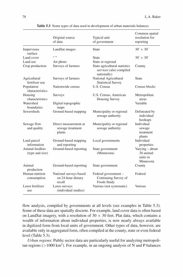
Public data sources: New tools and databases now make the development of materi-als flow analysis for large urban regions fairly practical. In particular, the widespreaduse of geographic information systems (GIS) by all levels of government mean thatmany types of data are readily available on a spatially discrete basis, allowing afacile GIS analyst to create numerous data layers within a selected watershed orother discrete region.

5.3.3 System Boundaries

An important consideration for analyzing materials flows through cities or partsof cities is definition of system boundaries. One commonly used boundary is awatershed, defined by topographic features. One advantage of using a watershedboundary is that it is relatively easy to define the boundaries. However, for ana-lyzing materials flows through cities, there are several disadvantages: (1) watermoves across topographically-defined watershed boundaries, particularly throughstorm sewers and sanitary sewers (Chapter 2), and (2) urban regions are not neatlybounded by watersheds. There also may be significant vertical movement of solutesvia groundwater, which may necessitate delineation of a separate groundwater sys-tem. Political entities (such as counties or cities) can also be used to define bound-aries. These have the advantage that many types of data are organized by politicalboundaries (Table 5.3), but suffer the disadvantage that political boundaries are gen-erally not closely related to anything that might be considered an “ecosystem”. It isnot necessary that “boundaries” be spatial. For example, in our analysis of house-hold ecosystems (Baker et al. 2007a), we developed a conceptual boundary thatincluded all activities of household members. By this definition, all driving and airtravel done by household members occurred within the boundary of the householdecosystem.

5.3.4 Scales of Analysis

MFA studies can be conducted at scales from individual households to entire urbanregions. Vast amounts of publicly available data are readily accessible for materials

78 L.A. Baker

Table 5.3 Some types of data used in development of urban materials balances

Common spatialOriginal source Typical unit resolution forof data of government reporting

Impervioussurface

LandSat images State 30′ × 30′

Land cover “ ” State 30′ × 30′

Land use Air photo State or regionalCrop production Surveys of farmers State agricultural statistics

services (also compilednationally)

County

Agriculturalfertilizer use

Surveys of farmers National AgriculturalStatistical Survey

State

Populationcharacteristics

Nationwide census U.S. Census Census blocks

Housingcharacteristics

Surveys U.S. Census, AmericanHousing Survey

Metropolitanareas

Watershedboundaries

Digital topographicmaps

Variable

Sewersheds Ground-based mapping Municipality or regionalsewage authority

Delineated byindividualhookups

Sewage flowand quality

Direct measurement atsewage treatmentplants

Municipality or regionalsewage authority

Individualsewagetreatmentplants

Land parcelinformation

Ground-based mappingand reporting

Local governments Individualproperties

Animal feedlots(type and size)

Ground-based reporting State government(Minnesota)

Varying – about30 animalunits inMinnesota

Animalproduction

Ground-based reporting State government County

Human nutrientconsumption

National surveys basedon 24-hour dietaryrecall

Federal government –Continuing Survey ofFoods Study

Federal

Lawn fertilizeruse

Lawn surveys(individual studies)

Various (not systematic) Various

flow analysis, compiled by governments at all levels (see examples in Table 5.3).Some of these data are spatially discrete. For example, land cover data is often basedon LandSat imagery, with a resolution of 30 × 30 feet. Plat data, which contains awealth of information about individual properties, is now nearly always availablein digitized form from local units of government. Other types of data, however, areavailable only in aggregated form, often compiled at the county, state or even federallevel (Table 5.3).

Urban regions: Public sector data are particularly useful for analyzing metropoli-tan regions (>1000 km2). For example, in an ongoing analysis of N and P balances


for the Twin Cities, Minnesota, we estimated the population of all U.S. Censusblocks located within the regional watershed, allowing a high degree of precision.Because the watershed comprised a large fraction of five counties, we could alsoconfidently utilize a wealth of data collected at the county level, on the assumptionthat per capita fluxes collected at the 5-county or regional level would be similar toper capita fluxes within the watershed.

Household scale: We have used a hybrid approach to study fluxes of materi-als through individual households (Baker et al. 2007a). In this study, we used acombination of an extensive questionnaire, plat data, data acquired from home-owners (energy bills and odometer readings) and landscape measurements. This isprobably the only way to collect information needed for materials balances for indi-vidual households with a reasonable degree of reliability.

Intermediate scales: Intermediate scales of analysis pose greater problems. Forexample, small watersheds (< ∼100 km2) may be a small part of a county orregional governmental unit. In this case, it may not be reasonable to assume thataverage characteristics of the watershed are similar to county to tabulated countyor regional characteristics. For example, the American Housing Survey compilesa wealth of data on household characteristics within metropolitan areas, but onecould not assume that average values for these characteristics (e.g., household sizeor energy cost) are averages for a particular study watershed. These problems mayovercome in the future, as more and more data are compiled and reported at finerspatial resolutions.

5.3.5 Indirect Fluxes

The issue of “indirect” fluxes of materials presents a problem that requires carefulboundary delineation. Indirect fluxes of materials are those that occur outside thesystem boundary, but are affected by activities within the system. For example, thecarbon flux used to manufacture a car may occur outside an urban ecosystem, butis affected by the purchase of cars within the system. Moreover, additional carbonfluxes occur outside the factory that manufactures the car – for example, as foodused to feed the workers at the plant. There is no entirely satisfactory solution tothis problem, but when indirect fluxes are being included in a MFA, the boundaryof indirect fluxes needs to be carefully defined.

5.3.6 Prior Studies

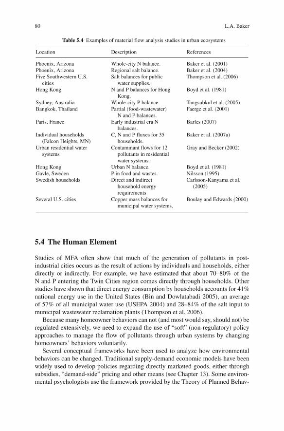
Methodologies for developing urban materials balances and MFA are rapidlyimproving as more researchers undertake these projects. Table 5.4 shows thatmost of these studies have dealt with water, nutrients, and salts. Studies on urbanmetabolism, which generally focus on energy and water, are reviewed by Kennedyet al. (2007).

80 L.A. Baker

Table 5.4 Examples of material flow analysis studies in urban ecosystems

Location Description References

Phoenix, Arizona Whole-city N balance. Baker et al. (2001)Phoenix, Arizona Regional salt balance. Baker et al. (2004)Five Southwestern U.S.

citiesSalt balances for public

water supplies.Thompson et al. (2006)

Hong Kong N and P balances for HongKong.

Boyd et al. (1981)

Sydney, Australia Whole-city P balance. Tangsubkul et al. (2005)Bangkok, Thailand Partial (food-wastewater)

N and P balances.Faerge et al. (2001)

Paris, France Early industrial era Nbalances.

Barles (2007)

Individual households(Falcon Heights, MN)

C, N and P fluxes for 35households.

Baker et al. (2007a)

Urban residential watersystems

Contaminant flows for 12pollutants in residentialwater systems.

Gray and Becker (2002)

Hong Kong Urban N balance. Boyd et al. (1981)Gavle, Sweden P in food and wastes. Nilsson (1995)Swedish households Direct and indirect

household energyrequirements

Carlsson-Kanyama et al.(2005)

Several U.S. cities Copper mass balances formunicipal water systems.

Boulay and Edwards (2000)

5.4 The Human Element

Studies of MFA often show that much of the generation of pollutants in post-industrial cities occurs as the result of actions by individuals and households, eitherdirectly or indirectly. For example, we have estimated that about 70–80% of theN and P entering the Twin Cities region comes directly through households. Otherstudies have shown that direct energy consumption by households accounts for 41%national energy use in the United States (Bin and Dowlatabadi 2005), an averageof 57% of all municipal water use (USEPA 2004) and 28–84% of the salt input tomunicipal wastewater reclamation plants (Thompson et al. 2006).

Because many homeowner behaviors can not (and most would say, should not) beregulated extensively, we need to expand the use of “soft” (non-regulatory) policyapproaches to manage the flow of pollutants through urban systems by changinghomeowners’ behaviors voluntarily.

Several conceptual frameworks have been used to analyze how environmentalbehaviors can be changed. Traditional supply-demand economic models have beenwidely used to develop policies regarding directly marketed goods, either throughsubsidies, “demand-side” pricing and other means (see Chapter 13). Some environ-mental psychologists use the framework provided by the Theory of Planned Behav-


ior (TPB) and its derivatives (Ajzen 1991). The TPB seeks to understand underlyingattitudes that affect the intent to behave in a particular way. It has been has been usedto understand behavioral controls involved in recycling (Gamba and Oskamp 1994),household energy use (Lutzenhiser 1993), urban homeowners’ riparian vegetation(Shandas 2006), and lawn management (Baker et al., 2008). Communications the-ory, which examines how new ideas diffuse from innovation through broad adoption,has also been used to understand the adoption of agricultural erosion (Rogers 1995).

Experience has shown that soft policy approaches can change environmentalbehaviors. For example, curbside recycling in the U.S. increased from 7% of munic-ipal waste in the 1970s to 32% today (USEPA 2007). Farmland erosion declined by40% since the early 1980s (USDA 2003). Agricultural P fertilizer use has declinedby about 15% since the late 1970s, while yields have simultaneously increased (e.g.,corn yields over this period have more than doubled). Many urban water conserva-tion efforts have been successful (Renwick and Green 2000). Most of these pro-grams have included a mixture of policy tools. Typical elements include education,financial subsidies and/or disincentives, outright regulations (e.g. zoning, productbans restrictions) and social marketing. Some also target sensitive areas (e.g., erodi-ble land) or disproportionate consumers or polluters, such as flagrant householdwater consumers. These examples suggest that in the future, soft policies might alsobe used to reduce sources of urban stormwater pollution, alter diets to reduce agri-cultural pollution, and reduce CO2 emissions.

5.5 Adaptive Management

As we seek solutions for nonpoint source pollution, we will also need new mod-els for decision-making. In the traditional top-down management approach to pointsource pollution control, the impact of various levels of pollution reduction neededto achieve an environmental goal can readily be predicted using mathematical mod-els. For example, engineers can now readily predict the increase in oxygen levelsthat will occur in a river as the result of decreased inputs of BOD from sewage. Wealso have the ability to design sewage treatment plants to precisely achieve a specificBOD load reduction – no more and no less than required to achieve specific oxygenlevel (usually a legally mandated standard). Decision-making is therefore relativelystraightforward, with predictable outcomes and well-defined costs.

Managing the diffuse movement of pollutants through urban ecosystems is moreproblematic for several reasons: (1) pollution removal efficiencies for BMPs arehighly variable (2) mathematical models to represent diffuse pollution are not highlydeveloped, and (3) even if they were, obtaining accurate input data would be expen-sive and in some cases, nearly impossible (e.g., we have no good way to measurehow much fertilizer individual homeowners apply to lawns). One potential solutionis adaptive management, which involves making environmental measurements overlong periods, providing feedback to those involved in management, who changemanagement practices in response to feedback (Gunderson and Holling 2002). An

82 L.A. Baker

example of adaptive management that we are all familiar with is our weather fore-casting system. Our government policy to protect citizens from severe weather is toprovide continuous forecasts and measurements. The actual response by citizens isentirely unregulated: Each citizen listening to weather forecasts decides whether tocarry an umbrella if the forecast shows a 70% chance of rain. A person may choosenot to carry an umbrella when heavy rain is predicted, but over time, most peoplelearn that this is a good idea – they adapt. Generally the response is not based onraw data, but requires some level of interpretation and recommendation. The publicis interested in weather forecasts, not real-time barometer readings.

Very little water quality management in cities is currently based on adaptive man-agement, but several technological and cultural developments favor broader use ofadaptive management in the future. Some of these include: (1) rapidly improving,less expensive monitoring approaches, including citizen-based programs, to providefeedback; (2) increasing internet connectivity, which allows participants to receivefeedback and management recommendations, (3) the advent of “Web 2.0”, whichallows online dialogues, (4) growing environmental awareness and willingness tochange behaviors, and (5) a resurgent interest in citizen participation in governance.

5.6 Applications

This section examines several case studies of pollution management that involveMFA, social tools, and adaptive management to illustrate new directions in manage-ment of urban pollution.

5.6.1 Case Study 1: Urban Lawns and P Pollution

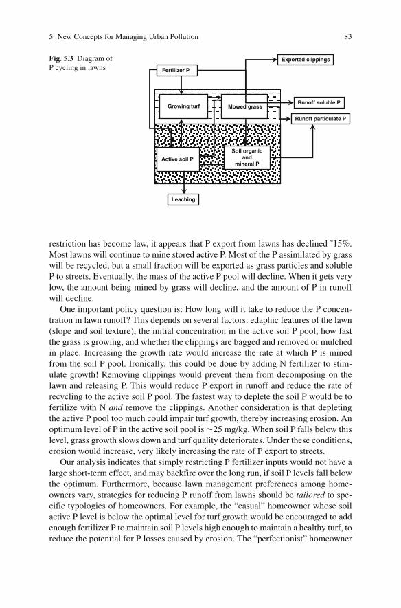
Lawn runoff typically contains 0.5–2.0 mg P/L, compared with levels around 0.1 mgP/L that typically result in lake eutrophication. Hence, lawns are probably the majorsource of P to stormwater in residential areas (Baker et al. 2007b). It would thereforebe desirable to develop policies that would reduce P export from residential lawns.Targeted lawn management strategies could be based on MFA of lawn P cycling(Fig. 5.3). Logical system boundaries would be the horizontal borders of the lawn(x–y axis) and the lawn surface down to the bottom of the root zone (z-axis). Somelawn P fertilizer is lost immediately as surface runoff, but this loss is typically <5%of applied P (reviewed by Baker et al. 2007b). Most of the applied P is assimilatedby grass or enters the soil. Because most urban lawns have been fertilized with P formany years, many have accumulated a large pool of active P that can be “mined” bygrowing turf for many years following cessation of fertilizer P inputs. When grass ismowed, some enters streets as P-containing particles and the rest decomposes on thelawn, releasing soluble P, which can become runoff or leach downward, replenishingthe active P pool.

One policy option would be to restrict the use of lawn P fertilizers, as the Min-nesota and several counties and cities have done. In the first few years since the


Growing turf

Active soil P

Soil organicand

mineral P

Fertilizer P

Runoff soluble P

Runoff particulate P

Exported clippings

Mowed grass

Leaching

Fig. 5.3 Diagram ofP cycling in lawns

restriction has become law, it appears that P export from lawns has declined ˜15%.Most lawns will continue to mine stored active P. Most of the P assimilated by grasswill be recycled, but a small fraction will be exported as grass particles and solubleP to streets. Eventually, the mass of the active P pool will decline. When it gets verylow, the amount being mined by grass will decline, and the amount of P in runoffwill decline.

One important policy question is: How long will it take to reduce the P concen-tration in lawn runoff? This depends on several factors: edaphic features of the lawn(slope and soil texture), the initial concentration in the active soil P pool, how fastthe grass is growing, and whether the clippings are bagged and removed or mulchedin place. Increasing the growth rate would increase the rate at which P is minedfrom the soil P pool. Ironically, this could be done by adding N fertilizer to stim-ulate growth! Removing clippings would prevent them from decomposing on thelawn and releasing P. This would reduce P export in runoff and reduce the rate ofrecycling to the active soil P pool. The fastest way to deplete the soil P would be tofertilize with N and remove the clippings. Another consideration is that depletingthe active P pool too much could impair turf growth, thereby increasing erosion. Anoptimum level of P in the active soil pool is ∼25 mg/kg. When soil P falls below thislevel, grass growth slows down and turf quality deteriorates. Under these conditions,erosion would increase, very likely increasing the rate of P export to streets.

Our analysis indicates that simply restricting P fertilizer inputs would not have alarge short-term effect, and may backfire over the long run, if soil P levels fall belowthe optimum. Furthermore, because lawn management preferences among home-owners vary, strategies for reducing P runoff from lawns should be tailored to spe-cific typologies of homeowners. For example, the “casual” homeowner whose soilactive P level is below the optimal level for turf growth would be encouraged to addenough fertilizer P to maintain soil P levels high enough to maintain a healthy turf, toreduce the potential for P losses caused by erosion. The “perfectionist” homeowner

84 L.A. Baker

with very high soil P levels needs to know that there is no benefit in maintaining theactive soil P level above the optimal level. In both cases, P fertilization should beadaptive, based on actual measurements of their lawn’s soil P levels. This testing isinexpensive, generally provided by university extension services.

Taken to the next level, quantitative modeling of lawn runoff could be used todetermine specific circumstances (slope, soil texture) where runoff P is most likelyproblematic. Watershed managers could then target their efforts on these areas.Homeowners in these areas would learn that they happen to be located on vulner-able areas. The TPB (discussed above) suggests that this type of specific, credibleknowledge would likely cause a greater change in homeowners’ behaviors than gen-eral guidance. Thus, a homeowner who is asked to change his lawn managementpractices because his lawn is particularly vulnerable – for example, on a steep slopewith clayey soils, where runoff can be 25% of precipitation – is more likely to adoptspecific advice than a random homeowner given generic advice.

5.6.2 Case Study 2: Using MFA to Devise Improved LeadReduction Strategy

Lead has probably been as harmful to human health in cities as any pollutant exceptperhaps fine particulate matter in air. Prior to the 1970s, two main inputs of leadto urban environments were leaded gasoline and lead-based paints, which togetheraccounted for ∼10–12 million tons of lead entering the environment. Both uses oflead were banned in the 1970s, leading to dramatic blood lead levels that parallelthe decline in use of leaded gasoline (Needleman 2004). Even so, the Center forDisease Control’s latest survey (1999–2002) shows that 1.6% of all children and3.1% of black children in the United States had blood lead levels (BLLs) greaterthan the “action limit” of 10 �g/dL. Symptoms of moderate lead poisoning includeirritability, inattention, and lower intelligence in children and hypertension in adults.The problem today is largely concentrated in poor, non-white urban populations. Forexample, more than 30% of the residents (all ages) in Baltimore City, Maryland hadelevated BLLs in the early 1990s (Silbergeld 1997). Urban lead poisoning thereforeremains a critical human health problem (Table 5.5).

Currently, lead hazard interventions to reduce blood lead levels in children havefocused on either abatement (removal of lead-based paint or contaminated soil) or

Table 5.5 Trend in BLLs > 10 �g/dL. Source: Centers for Disease Control

Percentage of children, ages 1–5, with BLLs >10 �g/dL

All races White, non-Hispanic Black, non-Hispanic

1976–1980 88.2 – –1988–1991 8.6 6 181991–1994 4.4 2.3 11.21999–2002 1.6 1.3 3.1


interim controls (paint stabilization, dust control). These programs have been onlymoderately successful, at best reducing blood lead levels by 25% and never reducingthem to �10 �g/dL (PTF 2000).

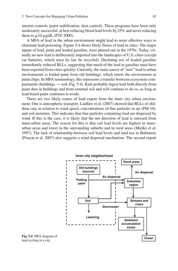
A MFA of lead in the urban environment might lead to more effective ways toeliminate lead poisoning. Figure 5.4 shows likely fluxes of lead in cities. The majorinputs of lead, paint and leaded gasoline, were phased out in the 1970s. Today, vir-tually no new lead is deliberately imported into the landscapes of U.S. cities (exceptcar batteries, which must by law be recycled). Declining use of leaded gasolineimmediately reduced BLLs, suggesting that much of the lead in gasoline must havebeen exported from cities quickly. Currently, the main source of “new” lead to urbanenvironments is leaded paint from old buildings, which enters the environment aspaint chips. In MFA terminology, this represents a transfer between ecosystem com-partments (buildings → soil; Fig. 5.4). Kids probably ingest lead both directly frompaint dust in buildings and from external soil and will continue to do so, as long aslead-based paint continues to erode.

There are two likely routes of lead export from the inner city urban environ-ment. One is atmospheric transport. Laidlaw et al. (2007) showed that BLLs of chil-dren vary in relation to wind speed, concentrations of fine particles in air (PM-10),and soil moisture. This indicates that fine particles containing lead are dispersed bywind. If this is the case, it is likely that the net direction of lead is outward frominner-urban areas. The reason for this is that soil lead levels are highest in inner-urban areas and lower in the surrounding suburbs and in rural areas (Mielke et al.1997). The lack of relationship between soil lead levels and land use in Baltimore(Pouyat et al. 2007) also suggests a wind dispersal mechanism. The second export

Old buildings(source)

Inner city neighborhood

Stormwater

Sedimentaccumulation

zones

Pealingpaint

Suburbanregion

Air dispersal

Rural areas

Leaching

Streams andrivers

Ocean

Air dispersal

Soil

Fig. 5.4 MFA diagram oflead cycling in a city

86 L.A. Baker

route is wash-off of wind-blown lead-laden dust that has settled on local impervi-ous surfaces (e.g., streets and sidewalks). Rain events transports lead to storm waterdrains. Kaushal et al. (2006) found that the mean lead concentration in storm waterfrom some Baltimore streams was 75 �g/L decades after new lead inputs had ceased,indicating that lead is slowly being exported by storm water. Storm sewers wouldtransport lead to low-lying sediment accumulation zones, such as stormwater deten-tion basins and stream riparian areas, where it would be deposited. Particle-boundlead would be transported further downstream during flood events to be re-depositedin regional rivers or transported to the ocean (Fig. 5.4). The one export route that isnot likely is downward leaching: Lead is tightly adsorbed to soil and is unlikely toleach.

The obvious means of reducing lead in the urban environment is careful removalor containment of lead-based paint, or removal or burial of entire buildings. Overtime, existing environmental lead would be reduced by export via wind and water.More detailed study of export mechanisms could lead to focused management toaccelerate removal of environmental lead. For example, frequent high-efficiencystreet sweeping and removal of highly contaminated soils might accelerate removalof accumulated lead, while also controlling the export route (to hazardous wastelandfills, rather than dispersal to outlying residential areas or to downstream aquaticecosystems).

5.6.3 Case Study 3: Managing Road Salt with AdaptiveManagement

De-icing roads using salt has accelerated over the past 40 years, increasing ten-foldsince the 1960s. Road salting has resulted in widespread contamination of streamsand groundwater in cold regions of the United States (Kaushal et al. 2005). Chlorideconcentrations in some urban areas can reach several thousand mg/L during peaksnowmelt periods, and can remain elevated above 250 mg/L even during base flowperiods, exceeding chronic water standards for protection of aquatic life. Chloridealso is highly mobile and can readily move through soils, contaminating aquifers.In the Shingle Creek watershed in Brooklyn Park, Minnesota, groundwater chlorideconcentrations have increased 10-fold, presumably due to road salt. Over the longterm road salt could potentially contaminate some urban aquifers to the point that thequality of groundwater would no longer be suitable for municipal water supply. Thepotential problem with reducing road salt use is increased potential for accidents,so reduction has to be done in a way that assures safe driving conditions. Somecommon strategies used to reduce the amount of salt applied include the use of pre-made brines rather than dry salt and the use of “pre-wetting” – application of saltor brine to the road before a major winter storm, rather than afterwards. Chlorideuse can be reduced through the use of alternative de-icers, such as calcium acetate,but these are generally far more expensive and may cause other problems (Novotnyet al. 1999).


Monitoring Analysis

Information tooperators

Modified saltingoperation

Initial salting operation

Fig. 5.5 Scheme of adaptive management for road de-icing

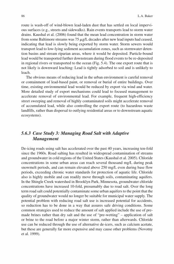
Adaptive management might be used to further reduce the amount of road saltused. Management of road salt is well-suited to an adaptive management, for the fol-lowing reasons: (1) road salt crews are a relatively small, captive audience, whichenables frequent communication, (2) because road salt is often overused, there ispotential for reduced use, hence savings, (3) several technologies can reduce theamount of salt needed, including pre-wetting, application of brine rather than drysalt and use of non-chloride alternative, and (4) chloride can be readily measuredindirectly, as conductivity – a method that is simple, inexpensive, reliable and read-ily automated, enabling real-time monitoring on pavements, in storm sewers and instreams (Baker 2007). The essential elements of an adaptive management schemefor road de-icing are shown in Fig. 5.5.

Requisite data to guide road de-icing management could readily be obtained viaenvironmental sensors. Road surface temperature and specific conductance (a sur-rogate measurement for chloride) could readily be measured at the road surface andin streams. Precipitation amount for each event could be interpolated from mea-sured precipitation at weather networks. Newer salting trucks have computerizedequipment to record the mass of salt used per mile. Analysis of data from a seriesof de-icing events might include simple statistical analysis, hydrologic modeling orother methods. In addition, adaptive management often uses human feedback – inthis case, the perceptions and knowledge of the salt truck operators. This analysiswould be used to guide subsequent de-icing operations, which in turn would resultin new data for analysis. This cycle would continue, with the goal of improvingde-icing operations until environmental and safety goals are met.

5.7 Summary

Creating sustainable, resilient urban ecosystems requires that we understand andmanage the flow of polluting materials through them. From the time of early indus-trialization through the 20th century, we rarely analyzed the flows of these materials,

88 L.A. Baker

often with disastrous, or at least, unpleasant effects. For example, allowing urbanlead pollution to occur, and allowing it to persist through the 1970s, will probablybe recorded by historians as one of the poorest environmental decisions in the 20thcentury. Today, MFA methods are sufficiently well developed that they can be usedto guide pollution management strategies. As a minimum, we can now develop rea-sonable a reasonable view of the movement of polluting materials through urbanregions. We can also expect that new databases, with more types of data and at finerresolution, will enable even broader applications.

Many of the findings from MFA analysis will likely point toward “soft” and poli-cies to change environmental behaviors of ordinary citizens. To do this, we also needto understand how people make environmental decisions. This will require a newdegree of interdisciplinary collaboration to develop transdisciplinary knowledge ofsocial–ecological systems. This type of thinking has largely been missing from mostpollution management policy, with the exception of economic cost-benefit analysis.One very promising approach that integrates the biophysical and social realms isadaptive management. New technologies enable a whole new realm of feedbackmechanisms to inform policy makers at all levels, including individual citizens. Weexamined case studies involving lawn runoff, urban lead pollution and road salt toillustrate these concepts.

MFA may have particular importance for cities in arid lands, because contami-nants in water tend to be retained in arid cities, rather than flushed from cities, aswould be the case for wetter regions. Water conservation measures in general, andrecycling of wastewater in particular, tend to exacerbate accumulation of solutessuch as salt and nitrate within the urban ecosystem, especially in underlying aquifers(Chapter 4, Baker et al. 2004). Although cities in arid lands have persisted for thou-sands of years, historical per capita water use rates were probably very low, so accu-mulation of solutes would have been slow. In the modern, post-industrial city, soluteaccumulation is accelerated by very high water use, often several hundred gallonsper person per day and the long-term consequences have not been studied. Becausemost of the world’s population increase is occurring in cities in arid lands, managingthe flow of materials through them may be essential for sustainability.

Acknowledgements Research reported in this chapter was supported by NSF BiocomplexityProjects 0322065 and 0709581 to L. Baker.

References

Ajzen, I. 1991. The theory of planned behavior. Organizational Behavior and Human DecisionProcesses 50:179–211.

Baker, L. A. 2007. Stormwater pollution: getting at the source. Storm Water 8 (Nov. 2007),http://www.stormh2o.com/november-december-2007/bmps-ms4-pollution.aspx

Baker, L. A., B. Wilson, D. Fulton, and B. Horgan. Disproportionality as a framework for urbanlawn management. Cities and the Environment. Cities and the Environment 1:2 Article 7.

Baker, L. A., and P. L. Brezonik. 2007. Using whole-system mass balances to craft novelapproaches for pollution reduction: examples at scales from households to urban regions, pp.92–104. In: V. Novotny and P. R. Brown, editors. Cities of the Future: Toward Integrated


Sustainable Water and Landscape Management. Proceedings of a conference held at theWingspan Center, Racine, WI (USA), July 12–14, 2006. IWA Publishing, London.

Baker, L. A., P. Hartzheim, S. Hobbie, J. King, and K. Nelson. 2007a. Effect of consumptionchoices on flows of C, N and P in households. Urban Ecosystems 10:97–110.

Baker, L. A., R. Holzalksi, and J. Gulliver. 2007b. Source reduction, Chapter 7. In: J. A. Gulliverand J. Anderson, editors. Assessment of Stormwater Best Management Practices. MinnesotaWater Resources Center, St. Paul.

Baker, L. A., A. Brazel, and P. Westerhoff. 2004. Environmental consequences of rapid urbaniza-tion in warm, arid Lands: case study of phoenix, Arizona (USA), pp. 155–164. In: Marchettini,N., C. A. Brebbia, E. Tiezzi, and L. C. Wadhwa, editors. The Sustainable City III, WIT Press,Sienna, Italy.

Baker, L. A., Y. Xu, D. Hope, L. Lauver, and J. Edmonds. 2001. Nitrogen mass balance for thePhoenix-CAP ecosystem. Ecosystems 4:582–602.

Barles, S. 2007. Feeding the City: Food Consumption and Circulation of Nitrogen, Paris, 1801–1914. Science of the Total Environment 375: 48–58.

Bin, S. and H. Dowlatabadi. 2005. Consumer lifestyle approach to U.S. energy use and relatedCO2 emissions. Energy Policy 33: 197–208.

Borrud, L., E. Wilkinson, and S. Mickle. 1996. What we eat in America: USDA surveys foodconsumption changes. Foods Review 14–19.

Boulay, N., and M. Edwards. 2000. Copper in the urban water cycle. Crit. Reviews in Environmen-tal Science and Technology 30:297–326.

Boyd, S., S. Millar, K. Newcombe, and B. O′Neill. 1981. The Ecology of a City and its People:The Case of Hong Kong. Australian National University Press, Canberra, Australia.

Carlsson-Kanyama, A., R. Engstrom, and R. Kok. 2005. Indirect and direct energy requirementsof city households in Sweden. Journal of Industrial Ecology 9:221–235.

Faerge, J., J. Magid, and W. T. Penning de Vries. 2001. Urban nutrient balance for Bangkok.Ecological Modeling 139:63–74.

Gamba, R. J., and S. Oskamp. 1994. Factors influencing community residents participation incomingled curbside recycling programs. Environment and Behavior 126:587–612.

Goolsby, D. A., and W. A. Battaglin. 2001. Long-term changes in concentrations and flux of nitro-gen in the Mississippi River Basin, USA. Hydrological Processes 15:1209–1226.

Gray, S. R., and N. S. C. Becker. 2002. Contaminant flows in urban residential water systems.Urban Water 4:331–346.

Gunderson, L. H., and C. S. Holling. 2002. Panarchy: understanding transformations in human andnatural systems. Island Press, Washington.

Hering, J. R., and J. R. Fantel. 1993. Phosphate rock demand into the next century: impact on worldfood supply. Natural Resources Research 2:226–246.

Kaushal, S. S., K. T. Belt, W. P. Stack, R. V. Pouyat, and P. M. Groffman. 2006. Variations in heavymetals across urban streams. EOS Transactions, Jt. Assem. Suppl. (abstract) 87.

Kaushal, S. S., P. M. Groffman, G. E. Likens, K. T. Belt, W. P. Stack, V. R. Kelly, L. E. Band,and G. T. Fisher. 2005. Increased salinization of fresh water in the northeastern United States.Proceedings of the National Academy Sciences 102:13517–13520.

Kennedy, C., J. Cuddihy, and J. Engel-Yan. 2007. The Changing Metabolism of Cities. Journal ofIndustrial Ecology 11:43–59.

Laidlaw, M. A. S., H. W. Mielke, G.M. Filippelli, D. L. Johnson, and C. R. Gonzoles. 2007. Sea-sonality and children′s blood lead levels: developing a predictive model using climatic vari-ables and blood lead data from Indianapolis, Indiana, Syracuse, New York, and New Orleans,Louisiana (USA). Environmental Health Perspectives 113:793–800.

Lauver, L., and L. A. Baker. 2000. Nitrogen mass balance for wastewater in the Phoenix-Central Arizona Project ecosystem: implications for water management. Water Research 34:2754–2760.

Lutzenhiser, L. 1993. Social and behavioral aspects of energy use. Annual Review of Energy andthe Environment 18:247–289.

90 L.A. Baker

Metcalf, and Eddy. 1991. Wastewater engineering: treatment, disposal, and reuse. McGraw-Hill,New York.

Mielke, H. W., D. Dugs, P. W. Mielke, K. S. Smith, S. L. Smith, and C. R. Gonzoles. 1997. Asso-ciations between soil lead and childhood blood lead in urban New Orleans and rural LafourcheParish of Louisiana. Environmental Health Perspectives 105:950–954.

Milesi, C., C. D. Elvidge, J. B. Dietz, B. T. Tuttle, R. N. Ramkrishna, and S. W. Running. 2005.Mapping and modeling the biogeochemical cycling of turf grasses in the United States. Journalof Environmental Management 36:426–438.

Miyamoto, S., J. White, R. Bader, and D. Ornelas. 2001. El Paso Guidelines for Landscape Usesof Reclaimed Water with Elevated Salinity. El Paso Public Utilities Board, Water Services, ElPaso.

Needleman, H. 2004. Lead poisoning. Annual Review of Medicine 55:209–222.Nilsson, J. 1995. A phosphorus budget for a Swedish municipality. Journal of Environmental Man-

agement 45:243–253.Novotny, V., D. W. Smith, D. A. Duemmel, J. Mastriano, and A. Bartosova. 1999. Urban and

Highway Snowmelt: Minimizing the Impact on Receiving Water. Water Environment ResearchFoundation, Alexandria, VA.

Pouyat, R. V., I. D. Yesilonis, J. Russell-Anelli, and N. K. Neerchal. 2007. Soil chemical andphysical properties that differentiate urban land-use and cover types. Soil Science Society ofAmerica Journal 71:1010–1019.

PTF. 2000. Eliminating Childhood Lead Poisoning: A Federal Strategy Targetting Lead Paint Haz-ards. President′s Task Force on Environmental Health Risks and Safety Risks to Children,Washington, DC.

Puckett, L. J. 1995. Identifying the major sources of nutrient water pollution. Environmental Sci-ence Technology 29:408–414.

Qian, Y. L., W. W. Bandaranayake, W. J. Parton, B. Mecham, M. A. Harivandi, and A. Mosier.2003. Long-term effects of clipping and nitrogen amendment on management in turfgrass onsoil organic carbon and nitrogen dynamics: the CENTURY model simulation. Journal of Envi-ronmental Quality 32:694–1700.

Reed, S. C., R. W. Crites, and E. J. Middlebrooks. 1995. Natural Systems for Waste Managementand Treatment. McGraw-Hill, New York.

Renwick, M. E., and R. D. Green. 2000. Do residential water demand side management policiesmeasure up? An analysis of eight California water management agencies. Journal of Environ-mental Economics and Managment 40:37–55.

Rogers, E. 1995. Diffusion of Innovations (4th ed.). Free Press, New York.Shandas, V. 2006. An empirical study of streamside landowners′ interest in riparian conservation.

Journal of the American Planning Association 73:173–183.Silbergeld, E. K. 1997. Preventing lead poisoning in children. Annual Review of Public Health

18:187–210.Smil, V. 2000. Phosphorus in the environment: natural flows and human interferences. Annual

Review Energy and Environment 25:53–88.Smith, R. A., R. B. Alexander, and K. J. Lanfear. 1994. Stream Water Quality in the Conterminous

United States – Status and Trends of Selected Indicators During the 1980′s. National WaterSummary 1990–91 – Stream Water Quality Water-Supply Paper 2400, U.S. Geological Survey,Washington, DC.

Tangsubkul, N., S. Moore, and T. D. Waite. 2005. Incorporating phosphorus management consid-erations into wastewater management practice. Environmental Science & Policy 8:1–15.

Thompson, K., W. Christofferson, D. Robinette, J. Curl, L. A. Baker, J. Brereton, and K. Reich.2006. Characterizing and Managing Salinity Loadings in Reclaimed Water Systems. AmericanWater Works Research Foundation, Denver, CO.

USEPA. 2000a. Progress in Water Quality: An Evaluation of the National Investment in MunicipalWastewater Treatment. U.S. Environmental Protection Agency, Washington, DC.


USEPA. 2000b. National Water Quality Inventory: 2000. U.S. Environmental Protection Agency,Washington, DC.

USDA. 2003. 1997 erosion rates. Natural Resources Conservation Service, U.S. Department ofAgriculture, Washington, DC.

USEPA. 2004. How we use water in the United States. U.S. Environmental Protection Agency,Washington, DC.

USEPA. 2007. Recycling-basic facts. http://www.epa.gov/msw/facts.htmWeiss, P. T., J. S. Gulliver, and A. J. Erickson. 2007. Cost and pollutant removal of storm-water

treatment practices. Journal of Water Resources Planning and Management 133:218–229.

chapter 5 new concepts for managing urban pollution

Documents