chapter 5 contrasts for one-way anova 4. brand name ...• do english majors score differently than...
TRANSCRIPT
5-1 © 2006 A. Karpinski
Chapter 5 Contrasts for one-way ANOVA
Page 1. What is a contrast? 5-2 2. Types of contrasts 5-5 3. Significance tests of a single contrast 5-10 4. Brand name contrasts 5-22 5. Relationships between the omnibus F and contrasts 5-24 6. Robust tests for a single contrast 5-29 7. Effect sizes for a single contrast 5-32 8. An example 5-34 Advanced topics in contrast analysis 9. Trend analysis 5-39 10. Simultaneous significance tests on multiple contrasts 5-52 11. Contrasts with unequal cell size 5-62 12. A final example 5-70

5-2 © 2006 A. Karpinski
Contrasts for one-way ANOVA 1. What is a contrast?
• A focused test of means • A weighted sum of means • Contrasts allow you to test your research hypothesis (as opposed to the
statistical hypothesis)
• Example: You want to investigate if a college education improves SAT scores. You obtain five groups with n = 25 in each group: o High School Seniors o College Seniors
• Mathematics Majors • Chemistry Majors • English Majors • History Majors
o All participants take the SAT and scores are recorded
o The omnibus F-test examines the following hypotheses: 543210 : µµµµµ ====H
equal are s' allNot : i1 µH
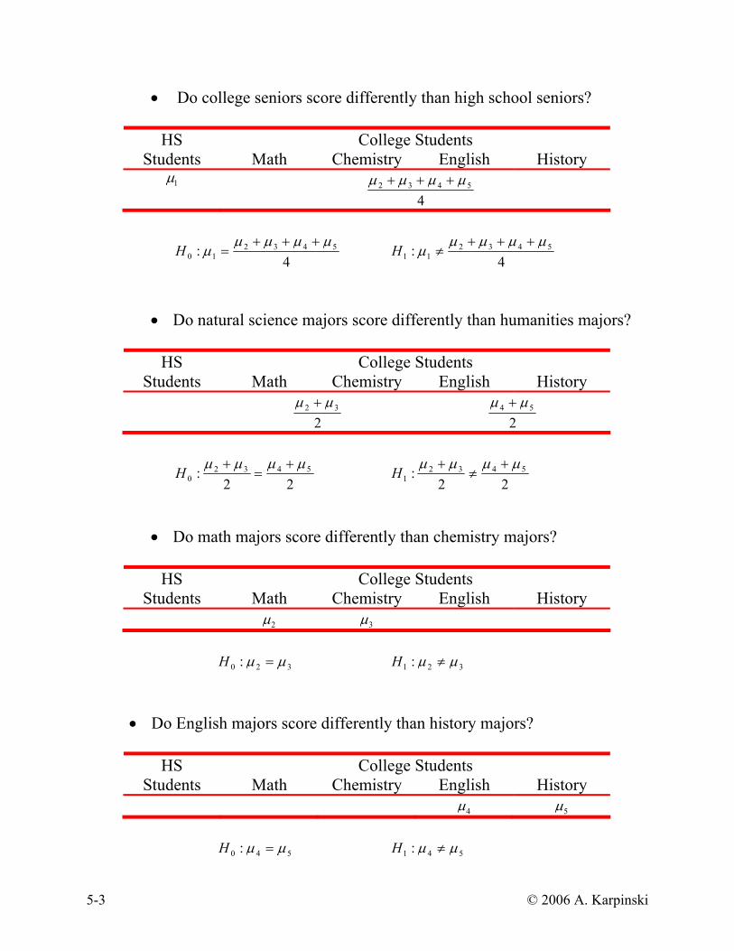
o But you want to know: • Do college seniors score differently than high school seniors? • Do natural science majors score differently than humanities majors? • Do math majors score differently than chemistry majors? • Do English majors score differently than history majors?
College Students HS
Students Math Chemistry English History µ1 µ2 µ3 µ4 µ5
5-3 © 2006 A. Karpinski
• Do college seniors score differently than high school seniors?
College Students HS Students Math Chemistry English History
µ1 4
5432 µµµµ +++
4: 5432
10µµµµ
µ+++
=H 4
: 543211
µµµµµ
+++≠H
• Do natural science majors score differently than humanities majors?
College Students HS Students Math Chemistry English History
2
32 µµ + 2
54 µµ +
22: 5432
0µµµµ +
=+
H 22
: 54321
µµµµ +≠
+H
• Do math majors score differently than chemistry majors?
College Students HS Students Math Chemistry English History
µ2 µ3
320 : µµ =H 321 : µµ ≠H
• Do English majors score differently than history majors?
College Students HS Students Math Chemistry English History
µ4 µ5
540 : µµ =H 541 : µµ ≠H

5-4 © 2006 A. Karpinski
• In general, a contrast is a set of weights that defines a specific comparison over the cell means
ψ = ciµi = c1µ1j =1
a
∑ + c2µ2 + c3µ3 + ...+ caµa
ˆ ψ = ciX i = c1X 1
j =1
a
∑ + c2 X 2 + c3 X 3 + ...+ ca X a
o Where
(µ1,µ2,µ3, ...,µa ) are the population means for each group (X 1, X 2,X 3, ...,X a ) are the observed means for each group (c1,c2,c3,...,ca )are weights/contrast coefficients
with cii=1
a
∑ = 0
• A contrast is a linear combination of cell means
o Do college seniors score differently than high school seniors?
4: 5432
10µµµµ
µ+++
=H or H0 : µ1 −µ2 + µ3 + µ4 + µ5
4= 0
543211 41
41
41
41 µµµµµψ −−−−=
−−−−=
41,
41,
41,
41,1c
o Do natural science majors score differently than humanities majors?
22: 5432
0µµµµ +
=+
H or H0 :µ2 + µ3
2−
µ4 + µ5
2= 0
54322 21
21
21
21 µµµµψ −−+=
−−=
21,
21,
21,
21,0c
o Do math majors score differently than chemistry majors?
320 : µµ =H or H0 : µ2 − µ3 = 0
323 µµψ −= ( )0,0,1,1,0 −=c

5-5 © 2006 A. Karpinski
2. Types of Contrasts
• Pairwise contrasts o Comparisons between two cell means o Contrast is of the form 1=ic and 1−=′ic for some i and i′
o If you have a groups then there are a(a −1)2
possible pairwise contrasts
o Examples: • Do math majors score differently than chemistry majors?
323 µµψ −= ( )0,0,1,1,0 −=c
• Do English majors score differently than history majors? 544 µµψ −= ( )1,1,0,0,0 −=c
o When there are two groups (a = 2), then the two independent samples t-
test is equivalent to the ( )1,1 −=c contrast on the two means.
• Complex contrasts o A contrast between more than two means o There are an infinite number of contrasts you can perform for any design
o Do college seniors score differently than high school seniors?
543211 41
41
41
41 µµµµµψ −−−−=
−−−−=
41,
41,
41,
41,1c
o Do natural science majors score differently than humanities majors?
54322 21
21
21
21 µµµµψ −−+=
−−=
21,
21,
21,
21,0c
o So long as the coefficients sum to zero, you can make any comparison:
54321 47.58.98.08.01. µµµµµψ ++−−=k ( )47,.58,.98.,08.,01. −−=c
• But remember you have to be able to interpret the result!
5-6 © 2006 A. Karpinski
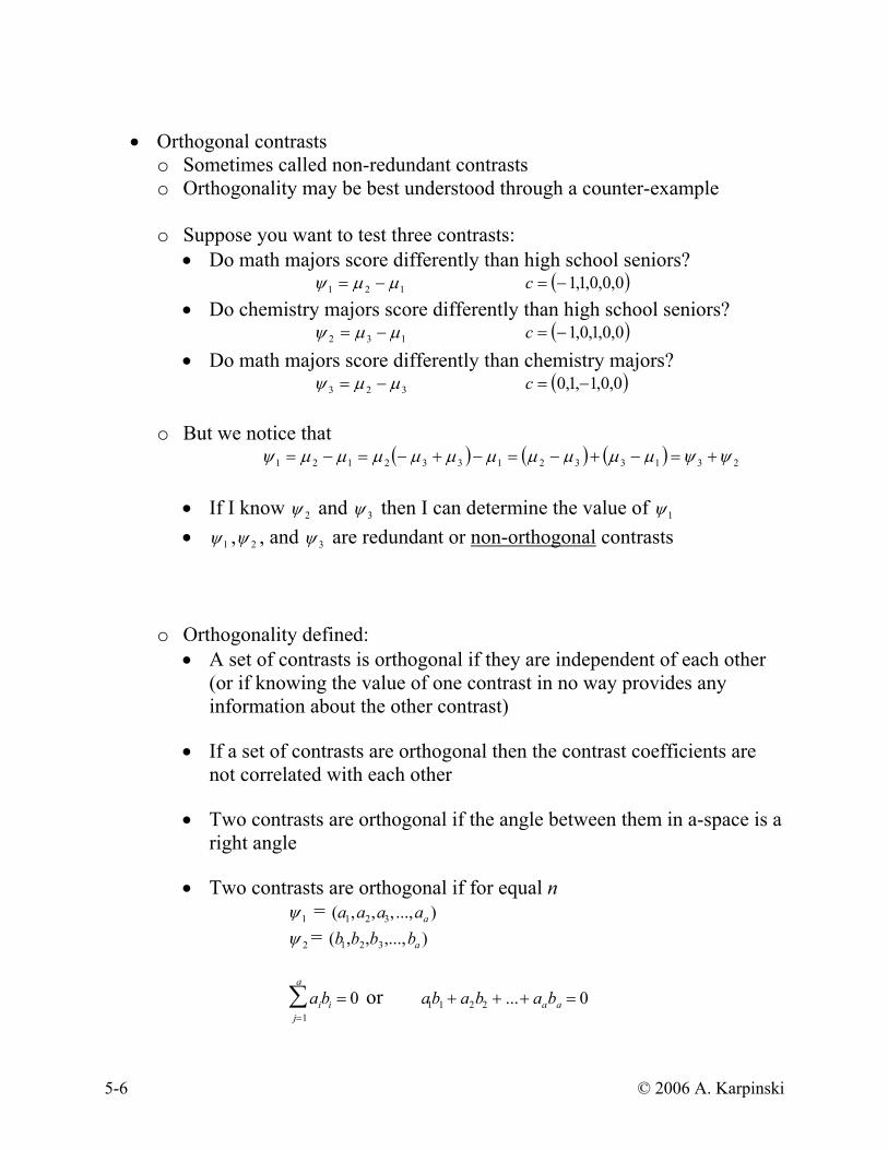
• Orthogonal contrasts
o Sometimes called non-redundant contrasts o Orthogonality may be best understood through a counter-example o Suppose you want to test three contrasts:
• Do math majors score differently than high school seniors? 121 µµψ −= ( )0,0,0,1,1−=c
• Do chemistry majors score differently than high school seniors? 132 µµψ −= ( )0,0,1,0,1−=c
• Do math majors score differently than chemistry majors? 323 µµψ −= ( )0,0,1,1,0 −=c
o But we notice that
( ) ( ) ( ) 2313321332121 ψψµµµµµµµµµµψ +=−+−=−+−=−=
• If I know 2ψ and 3ψ then I can determine the value of 1ψ • 1ψ , 2ψ , and 3ψ are redundant or non-orthogonal contrasts
o Orthogonality defined:
• A set of contrasts is orthogonal if they are independent of each other (or if knowing the value of one contrast in no way provides any information about the other contrast)
• If a set of contrasts are orthogonal then the contrast coefficients are
not correlated with each other
• Two contrasts are orthogonal if the angle between them in a-space is a right angle
• Two contrasts are orthogonal if for equal n
1ψ = (a1,a2,a3, ...,aa ) 2ψ = (b1,b2,b3,...,ba )
aibij=1
a
∑ = 0 or a1b1 + a2b2 + ...+ aaba = 0

5-7 © 2006 A. Karpinski
• Two contrasts are orthogonal if for unequal n
1ψ = (a1,a2,a3, ...,aa ) 2ψ = (b1,b2,b3,...,ba )
aibi
nij=1
a
∑ = 0 or a1b1
n1
+a2b2
n2
+ ...+aaba
na
= 0
o Examples of Orthogonality (assuming equal n)
• Set #1: ( )1,0,11 −=c and
−=
21,1,
21
2c
c1ic2ij=1
a
∑ = 1*12
+ 0 *−1( )+ −1*
12
= 12
+ 0 − 12
= 0 c1 and c2 are orthogonal
c1 ⊥ c2
• Set #2: ( )1,1,03 −=c and
−=
21,
21,14c
c3ic4 ij=1
a
∑ = 0 *−1( )+ 1*12
+ −1*
12
= 0 + 12
− 12
= 0 c3 and c4 are orthogonal
c3 ⊥ c4
• Set #3: ( )0,1,15 −=c and ( )1,0,16 −=c
c5ic6ij=1
a
∑ = 1*1( )+ −1*0( )+ 0 *−1( )
=1+ 0 + 0 =1
c5 and c6 are NOT orthogonal

5-8 © 2006 A. Karpinski
o A set of contrasts is orthogonal if each contrast is orthogonal to all other
contrasts in the set You can check that:
( )0,0,1,11 −=c 21 cc ⊥ ( )0,2,1,12 −=c 32 cc ⊥ ( )3,1,1,13 −=c 31 cc ⊥
o If you have a groups, then there are a-1 possible orthogonal contrasts
• We lose one contrast for the grand mean (the unit contrast) • Having the contrasts sum to zero assures that they will be orthogonal
to the unit contrast • If you have more than a-1 contrasts, then the contrasts are redundant
and you can write at least one contrast as a linear combination of the other contrasts
• Example: For a=3, we can find only 2 orthogonal contrasts. Any other
contrasts are redundant.
211 µµψ −= 1ψ ⊥ 2ψ
3212 21
21 µµµψ −+= 1ψ is not orthogonal to 3ψ
3213 51
54 µµµψ ++−= 2ψ is not orthogonal to 3ψ
We can write 3ψ in terms of 1ψ and 2ψ
213 51
109 ψψψ −−=
( )
−+−−−= 32121 2
121
51
109 µµµµµ
+−−+
+−= 32121 5
1101
101
109
109 µµµµµ
321 51
54 µµµ ++−=
• In general, you will not need to show how a contrast may be
calculated from a set of orthogonal contrasts. It is sufficient to know that if you have more than a-1 contrasts, there must be at least one contrast you can write as a linear combination of the other contrasts.

5-9 © 2006 A. Karpinski
o There is nothing wrong with testing non-orthogonal contrasts, as long as
you are aware that they are redundant. o For example, you may want to examine all possible pairwise contrasts.
These contrasts are not orthogonal, but they may be relevant to your research hypothesis.
• Nice properties of orthogonal contrasts: o We will learn to compute Sums of Squares associated with each contrast
(SSCi)
o For a set of a-1 orthogonal contrasts • Each contrast has one degree of freedom
SSB = SSC1 + SSC2 + SSC3 + . . . + SSCa-1 • In other words, a set of a-1 orthogonal contrasts partitions the SSB
• Recall that for the omnibus ANOVA, the dfbet = a −1. The omnibus test combines the results of these a-1 contrasts and reports them in one lump test
• Any set of a-1 orthogonal contrasts will yield the identical result as the omnibus test
5-10 © 2006 A. Karpinski
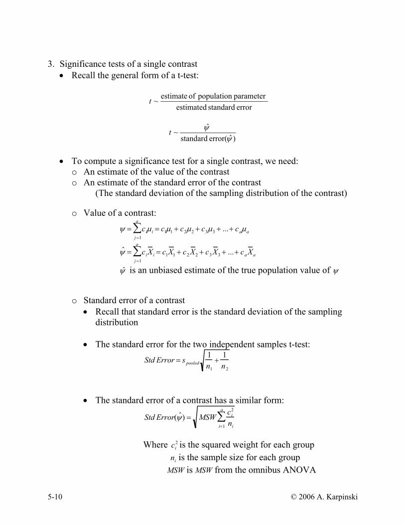
3. Significance tests of a single contrast
• Recall the general form of a t-test:
errorstandardestimatedparameter population of estimate~t
)ˆerror( standard ˆ
~ψ
ψt
• To compute a significance test for a single contrast, we need:
o An estimate of the value of the contrast o An estimate of the standard error of the contrast
(The standard deviation of the sampling distribution of the contrast)
o Value of a contrast:
ψ = ciµi = c1µ1j =1
a
∑ + c2µ2 + c3µ3 + ...+ caµa
ˆ ψ = ciX i = c1X 1j =1
a
∑ + c2 X 2 + c3 X 3 + ...+ ca X a
ψ̂ is an unbiased estimate of the true population value of ψ
o Standard error of a contrast • Recall that standard error is the standard deviation of the sampling
distribution • The standard error for the two independent samples t-test:
Std Error = s pooled1n1
+1n2
• The standard error of a contrast has a similar form:
Std Error( ˆ ψ ) = MSWci
2
nii=1
a
∑
Where 2
ic is the squared weight for each group in is the sample size for each group MSW is MSW from the omnibus ANOVA
5-11 © 2006 A. Karpinski
• Constructing a significance test
errorstandardestimatedparameter population of estimate~t
)ˆerror( standard ˆ
~ψ
ψt
o Now we can insert the parts of the t-test into the equation:
∑
∑=
i
i
iiobserved
nc
MSW
Xct
2
with degrees of freedom aNdf w −==
o To determine the level of significance, you can:
• Look up tcrit for df = N-a and the appropriate α • Or preferably, compare pobs with pcrit
o Note that because the test for a contrast is calculated using the t-
distribution, you can use either a one-tailed or two-tailed test of significance. As previously mentioned, you typically want to report the two-tailed test of the contrast.

5-12 © 2006 A. Karpinski
• Example #1: a=2 and ( )1,1 −=c
2121 )1()1(ˆ XXXX −=−+=ψ
Std error (ψ̂ ) = 212
2
1
2 11)1(1nn
MSWnn
MSW +=
−+
+
−==
21
21
11)ˆ(ˆ
nnMSW
XXStdError
tψ
ψ
o But we know that for two groups, MSW = spooled o Thus, the two independent samples t-test is identical to a ( )1,1 −=c
contrast on the two means
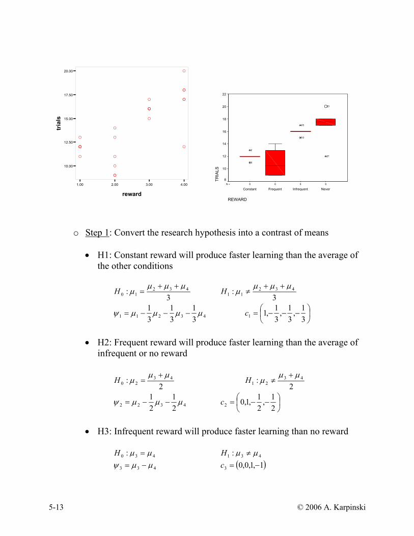
• Example #2: A study of the effects of reward on learning in children DV = Number of trials to learn a puzzle
Level of Reward
Constant (100%)
Frequent (66%)
Infrequent (33%)
Never (0%)
12 9 15 17 13 10 16 18 11 9 17 12 12 13 16 18 12 14 16 20 12 11 16 17
H1: Constant reward will produce faster learning than the average of the
other conditions H2: Frequent reward will produce faster learning than the average of
infrequent or no reward H3: Infrequent reward will produce faster learning than no reward
5-13 © 2006 A. Karpinski
1.00 2.00 3.00 4.00
reward
10.00
12.50
15.00
17.50
20.00
tria
ls
A
A
A
AAA
A
A
A
A
A
A
A
A
A
AAA
A
A
A
A
A
A
6666N =
REWARD
NeverInfrequentFrequentConstant
TRIA
LS
22
20
18
16
14
12
10
8
21
23
13
15
3
2
o Step 1: Convert the research hypothesis into a contrast of means
• H1: Constant reward will produce faster learning than the average of
the other conditions
3: 432
10µµµ
µ++
=H 3
: 43211
µµµµ
++≠H
43211 31
31
31 µµµµψ −−−=
−−−=
31,
31,
31,11c
• H2: Frequent reward will produce faster learning than the average of
infrequent or no reward
2: 43
20µµ
µ+
=H 2
: 4321
µµµ
+≠H
4322 21
21 µµµψ −−=
−−=
21,
21,1,02c
• H3: Infrequent reward will produce faster learning than no reward
430 : µµ =H 431 : µµ ≠H
433 µµψ −= ( )1,1,0,03 −=c

5-14 © 2006 A. Karpinski
o Step 2: Determine if the contrasts of interest are orthogonal
1c & 2c : ( ) 021*
31
21*
311*
310*1
4
121 =
−−+
−−+
−+=∑
=jiicc 1c ⊥ 2c
1c & 3c : ( ) 01*311*
310*
310*1
4
131 =
−−+
−+
−+=∑
=jiicc 1c ⊥ 3c
2c & 3c : ( ) ( ) 01*211*
210*10*0
4
132 =
−−+
−++=∑
=jiicc 2c ⊥ 3c
o Step 3: Compute values for each contrast
6667.2
)17(31)16(
31)11(
3112
31
31
31ˆ 43211
−=
−−−=
−−−= XXXXψ
5.5
)17(21)16(
21)11(
21
21ˆ 4322
−=
−−=
−−= XXXψ
1 )17()16(
ˆ 433
−=−=−= XXψ
o Step 4: Conduct omnibus ANOVA to obtain MSW
ANOVA Source of Variation SS df MS F P-value F crit Between Groups 130 3 43.33333 11.1828 0.000333 3.238867Within Groups 62 16 3.875 Total 192 19
• Note: we do not care about the results of this test. We only want to
calculate MSW

5-15 © 2006 A. Karpinski
o Step 5: Compute standard error for each contrast
Std Error( ˆ ψ ) = MSWci
2
nii=1
a
∑
Std err ( 1ψ̂ ) = 0165.12667.*875.3531
531
531
51875.3
222
2
==
−
+
−
+
−
+
Std err ( 2ψ̂ ) = ( ) 0782.130.*875.3521
521
510875.3
22
2
==
−
+
−
++
Std err ( 3ψ̂ ) = ( ) ( ) 2450.140.*875.351
5100875.3
22
==
−+++
o Step 6: Compute observed t or F statistic for each contrast
∑
∑=
i
i
iiobserved
nc
MSW
Xct
2
1ψ̂ : 6237.20165.16667.2
=−
=observedt 2ψ̂ : 1011.50782.1
5.5−=
−=observedt
3ψ̂ : 8032.02450.1
1−=
−=observedt
5-16 © 2006 A. Karpinski
o Step 7: Determine statistical significance
• Method 1 (The table method): Find tcrit for df = N-a and 025.205.
==α
tcrit (16)α=.025 = 2.12
Compare tcrit to tobs
if criticalobserved tt < then retain H0
if criticalobserved tt ≥ then reject H0
We reject the null hypothesis for 1ψ̂ and 2ψ̂
• Constant reward produced faster learning than the average of the other conditions
• Frequent reward produced faster learning than the average of infrequent or no reward
• Method 2: (The exact method): Find pobs for df = N-a and 025.205.
==α
for each tobs and Then compare pobs to pcrit = .05
1ψ : tobserved (16) = 2.62, p = .02 2ψ : tobserved (16) = −5.10, p < .01 3ψ : tobserved (16) = −0.80, p = .43
o Alternatively, you can perform an F-test to evaluate contrasts.
• We know that t2 = F
∑
∑=
i
i
iiobserved
nc
MSW
Xct
2
∑=
i
iobserved
nc
MSWF 2
2 ψ̂
df = N-a df = (1, N-a)
• You will obtain the exact same results with t-tests or F-tests.
5-17 © 2006 A. Karpinski
• Confidence intervals for contrasts
o In general, the formula for a confidence interval is ( ) error* standardtestimate critical±
o For a contrast, the formula for a confidence interval is
( ) error* standardtestimate critical±
± ∑
i
icritical n
cMSW * dfwt
2
)(ψ̂
• In the learning example, tcrit (16)α=.025 = 2.12
1ψ : ( )0165.112.2667.2 * ±− (-4.82, -0.51) 2ψ : ( )0782.112.25.5 * ±− (-7.79, -3.21)
3ψ : ( )2450.112.20.1 * ±− (-3.64, 1.64)
• Using SPSS to evaluate contrasts
o If you use ONEWAY, you can directly enter the contrast coefficients to obtain the desired contrast.
ONEWAY trials BY reward /STAT desc /CONTRAST = 1, -.333, -.333, -.333 /CONTRAST = 0, 1, -.5, -.5 /CONTRAST = 0, 0, 1, -1.

5-18 © 2006 A. Karpinski
Descriptives
TRIALS
5 12.0000 .70711 .31623 11.1220 12.87805 11.0000 2.34521 1.04881 8.0880 13.91205 16.0000 .70711 .31623 15.1220 16.87805 17.0000 3.00000 1.34164 13.2750 20.7250
20 14.0000 3.17888 .71082 12.5122 15.4878
ConstantFrequentInfrequentNeverTotal
N Mean Std. Deviation Std. Error Lower Bound Upper Bound
95% Confidence Interval forMean
Contrast Coefficients
1 -.333 -.333 -.3330 1 -.5 -.50 0 1 -1
Contrast123
Constant Frequent Infrequent NeverREWARD
Contrast Tests
-2.6520 1.01628 -2.610 16 .019-5.5000 1.07819 -5.101 16 .000-1.0000 1.24499 -.803 16 .434
Contrast123
Assume equal variancesTRIALS
Value ofContrast Std. Error t df Sig. (2-tailed)
o Multiplying the coefficients by a constant will not change the results of the significance test on that contrast. • If you multiply the values of a contrast by any constant (positive or
negative), you will obtain the identical test statistic and p-value in your analysis.
• The value of the contrast, the standard error, and the size of the CIs will shrink or expand by a factor of the constant used, but key features (i.e., p-values and whether or not the CIs overlap) remain the same.

5-19 © 2006 A. Karpinski
o Let’s examine Hypothesis 1 using three different sets of contrast
coefficients:
ONEWAY trials BY reward /STAT desc /CONTRAST = 1, -.333, -.333, -.333 /CONTRAST = 3, -1, -1, -1 /CONTRAST = -6, 2, 2, 2.
Contrast Coefficients
1 -.333 -.333 -.3333 -1 -1 -1
-6 2 2 2
Contrast123
Constant Frequent Infrequent NeverREWARD
Contrast Tests
-2.6520 1.01628 -2.610 16 .019-8.0000 3.04959 -2.623 16 .01816.0000 6.09918 2.623 16 .018
Contrast123
Assume equal variancesTRIALS
Value ofContrast Std. Error t df Sig. (2-tailed)
• You get more precise values if you enter the exact contrast coefficients into SPSS, so try to avoid rounding decimal places. Instead, multiply the coefficients by a constant so that all coefficients are whole numbers.
• In this case, the tests for contrasts 2 and 3 are exact. The test for contrast 1 is slightly off due to rounding.
5-20 © 2006 A. Karpinski
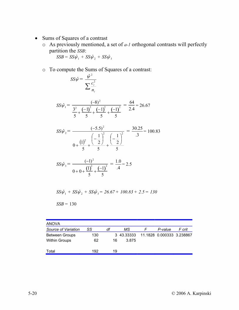
• Sums of Squares of a contrast
o As previously mentioned, a set of a-1 orthogonal contrasts will perfectly partition the SSB:
SSB = SS 1ψ̂ + SS 2ψ̂ + SS 3ψ̂
o To compute the Sums of Squares of a contrast:
SSψ̂ = ∑
i
i
nc 2
2 ψ̂
SS 1ψ̂ = (−8)2 32
5+
−1( )2
5+
−1( )2
5+
−1( )2
5
= 642.4
= 26.67
SS 2ψ̂ =
( )521
521
510
)5.5(22
2
2
−
+
−
++
− = 3.25.30 = 100.83
SS 3ψ̂ = (−1)2
0 + 0 +1( )2
5+
−1( )2
5
= 4.0.1 = 2.5
SS 1ψ̂ + SS 2ψ̂ + SS 3ψ̂ = 26.67 + 100.83 + 2.5 = 130 SSB = 130
ANOVA Source of Variation SS df MS F P-value F crit Between Groups 130 3 43.33333 11.1828 0.000333 3.238867Within Groups 62 16 3.875 Total 192 19

5-21 © 2006 A. Karpinski
o Once we have calculated the SSC, then we can compute an F-test directly:
MSWSSC
dfwSSW
dfcSSC
dfwF ==),1(
1ψ̂ : Fobserved =26.673.875
= 6.88 2ψ̂ : 021.26875.3
83.100==observedF
3ψ̂ : 645.0875.350.2
==observedF
o ANOVA table for contrasts
ANOVA Source of Variation SS df MS F P-value
Between Groups 130 3 43.33333 11.1828 0.000333 1ψ̂ 26.67 1 26.37 6.8817 0.018446 2ψ̂ 100.83 1 100.83 26.021 0.000107 3ψ̂ 2.50 1 2.50 0.645 0.433675 Within Groups 62 16 3.875 Total 192 19
• In this ANOVA table, we show that SSC partitions SSB. • But this relationship only holds for sets of orthogonal contrasts • In general, you should only construct an ANOVA table for a set of a-1
orthogonal contrasts
• Note: We will shortly see they you can either perform the omnibus test OR tests of orthogonal contrasts, but not both. Nevertheless, this ANOVA table nicely displays the SS partition.

5-22 © 2006 A. Karpinski
4. Brand name contrasts easily obtained from SPSS • Difference contrasts • Helmert contrasts • Simple contrasts • Repeated contrasts • Polynomial contrasts (to be covered later)
• Difference contrasts: Each level of a factor is compared to the mean of the previous levels (These are orthogonal with equal n)
c1 c2 c3 c4 -1 1 0 0 -1 -1 2 0 -1 -1 -1 3
Contrast Coefficients (L' Matrix)
.000 .000 .000-1.000 -.500 -.3331.000 -.500 -.333
.000 1.000 -.333
.000 .000 1.000
ParameterIntercept[REWARD=1.00][REWARD=2.00][REWARD=3.00][REWARD=4.00]
Level 2 vs.Level 1
Level 3 vs.Previous
Level 4 vs.Previous
REWARD Difference Contrast
The default display of this matrix is the transpose of thecorresponding L matrix.
UNIANOVA trials BY reward /CONTRAST (reward)=difference /PRINT = test(lmatrix)
5-23 © 2006 A. Karpinski
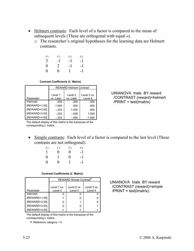
• Helmert contrasts: Each level of a factor is compared to the mean of
subsequent levels (These are orthogonal with equal n). o The researcher’s original hypotheses for the learning data are Helmert
contrasts.
c1 c2 c3 c4 3 -1 -1 -1 0 2 -1 -1 0 0 1 -1
Contrast Coefficients (L' Matrix)
.000 .000 .0001.000 .000 .000-.333 1.000 .000-.333 -.500 1.000-.333 -.500 -1.000
ParameterIntercept[REWARD=1.00][REWARD=2.00][REWARD=3.00][REWARD=4.00]
Level 1vs. Later
Level 2vs. Later
Level 3 vs.Level 4
REWARD Helmert Contrast
The default display of this matrix is the transpose of thecorresponding L matrix.
UNIANOVA trials BY reward /CONTRAST (reward)=helmert /PRINT = test(lmatrix)
• Simple contrasts: Each level of a factor is compared to the last level (These
contrasts are not orthogonal). c1 c2 c3 c4 1 0 0 -1 0 1 0 -1 0 0 1 -1
Contrast Coefficients (L' Matrix)
0 0 01 0 00 1 00 0 1
-1 -1 -1
ParameterIntercept[REWARD=1.00][REWARD=2.00][REWARD=3.00][REWARD=4.00]
Level 1 vs.Level 4
Level 2 vs.Level 4
Level 3 vs.Level 4
REWARD Simple Contrasta
The default display of this matrix is the transpose of thecorresponding L matrix.
Reference category = 4a.
UNIANOVA trials BY reward /CONTRAST (reward)=simple /PRINT = test(lmatrix).
5-24 © 2006 A. Karpinski
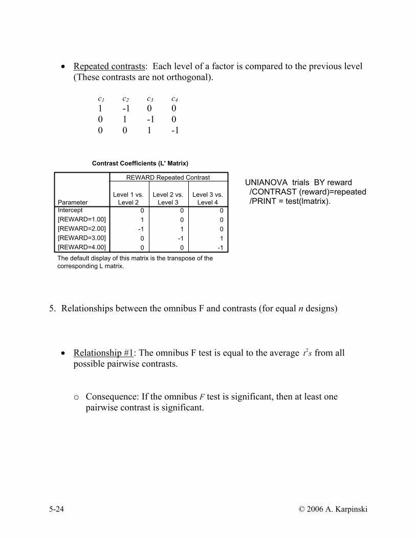
• Repeated contrasts: Each level of a factor is compared to the previous level
(These contrasts are not orthogonal).
c1 c2 c3 c4 1 -1 0 0 0 1 -1 0 0 0 1 -1
Contrast Coefficients (L' Matrix)
0 0 01 0 0
-1 1 00 -1 10 0 -1
ParameterIntercept[REWARD=1.00][REWARD=2.00][REWARD=3.00][REWARD=4.00]
Level 1 vs.Level 2
Level 2 vs.Level 3
Level 3 vs.Level 4
REWARD Repeated Contrast
The default display of this matrix is the transpose of thecorresponding L matrix.
UNIANOVA trials BY reward /CONTRAST (reward)=repeated /PRINT = test(lmatrix).
5. Relationships between the omnibus F and contrasts (for equal n designs)
• Relationship #1: The omnibus F test is equal to the average t2s from all possible pairwise contrasts.
o Consequence: If the omnibus F test is significant, then at least one pairwise contrast is significant.

5-25 © 2006 A. Karpinski
• Relationship #2: If you take the average F (or t2s) from a set of a-1
orthogonal contrasts, the result will equal the omnibus F!
o A mini-proof:
For 1ψ̂ : MSWSS
dfwSSW
dfSS
F 11
1
1
ˆˆˆ
ψψψ
== . . . . For ˆ ψ a−1 : Fa−1 =
SS ˆ ψ a−1df ˆ ψ a−1
SSWdfw
=SS ˆ ψ a−1
MSW
F =F1 + F2 + ...+ Fa−1
a −1=
SS ˆ ψ 1MSW
+ SS ˆ ψ 2MSW
+ ...+ SS ˆ ψ a−1
MSW
a −1
=
SS ˆ ψ 1 + SS ˆ ψ 2 + ...+ SS ˆ ψ a−1
MSW
a −1
=
SSBMSW
a −1 =
SSBa −1
MSW =
MSWMSB = omnibusF
o Consequence: If the omnibus F test is significant, then at least one contrast is significant.

5-26 © 2006 A. Karpinski
o In the learning example:
ANOVA
Source of Variation SS df MS F P-value Between Groups 130 3 43.33333 11.1828 0.000333 1ψ̂ 26.37 1 26.37 6.8052 0.019003 2ψ̂ 100.83 1 100.83 26.021 0.000107 3ψ̂ 2.50 1 2.50 0.645 0.433675 Within Groups 62 16 3.875 Total 192 19
• Average F from the set of orthogonal contrasts:
16.113
645.021.268052.6=
++ (Difference is due to rounding error)
• Is it possible to have a significant contrast, but have a non-significant omnibus F?
YES!
o Let’s consider an example:
IV Level 1 Level 2 Level 3 Level 4
1 2 2 4 2 3 3 5 3 4 4 6 4 5 5 7 5 6 6 8 3 4 4 6

5-27 © 2006 A. Karpinski
ONEWAY dv BY iv /CONTRAST= -1 -1 -1 3.
ANOVA
DV
23.750 3 7.917 3.167 .05340.000 16 2.50063.750 19
Between GroupsWithin GroupsTotal
Sum ofSquares df Mean Square F Sig.
o Omnibus F-test is not significant
Contrast Tests
7.0000 2.44949 2.858 16 .011Contrast1Assume equal variancesDV
Value ofContrast Std. Error t df Sig. (2-tailed)
o The contrast comparing Group 4 to the average of the other groups is significant
• Suppose none of the pairwise contrasts are significant. Is it possible to have a significant contrast?
YES!
o If none of the pairwise contrasts are significant, then the omnibus F test will not be significant. But you may still find a contrast that is significant!
IV
Level 1 Level 2 Level 3 Level 4 0 2 2 1 1 3 3 2 2 4 4 3 3 5 5 4 4 6 6 5 2 4 4 3

5-28 © 2006 A. Karpinski
ONEWAY dv BY iv /CONTRAST= 1 -1 0 0 /CONTRAST= 1 0 -1 0 /CONTRAST= 1 0 0 -1 /CONTRAST= 0 1 -1 0 /CONTRAST= 0 1 0 -1 /CONTRAST= 0 0 -1 1.
o None of the pairwise contrasts are significant:
Contrast Tests
-2.0000 1.00000 -2.000 16 .063-2.0000 1.00000 -2.000 16 .063-1.0000 1.00000 -1.000 16 .332
.0000 1.00000 .000 16 1.0001.0000 1.00000 1.000 16 .332
-1.0000 1.00000 -1.000 16 .332
Contrast123456
DV
Value ofContrast Std. Error t df Sig. (2-tailed)
o So we know that the omnibus F-test is not significant: ANOVA
DV
13.750 3 4.583 1.833 .18240.000 16 2.50053.750 19
Between GroupsWithin GroupsTotal
Sum ofSquares df Mean Square F Sig.
o But it is still possible to find a significant contrast: ONEWAY dv BY iv /CONTRAST= 1 -1 -1 1.
Contrast Tests
-3.0000 1.41421 -2.121 16 .050Contrast1DV
Value ofContrast Std. Error t df Sig. (2-tailed)

5-29 © 2006 A. Karpinski
• To reiterate:
o A significant omnibus F-test ⇒ There will be at least 1 significant
contrast
o A significant contrast DOES NOT IMPLY a significant omnibus F-test
o A non significant omnibus F-test DOES NOT IMPLY all contrasts will be non-significant
6. Robust tests for a single contrast
• The assumptions for contrasts are the same as those for ANOVA o Independent samples o Within each group, participants are independent and randomly selected o Equal population variances in each group o Each group is drawn from a normal population
• Tests of contrasts are not robust to heterogeneity of variances, even with
equal n
• We can use our standard ANOVA techniques to test these assumptions. Presumably, by the time you are testing contrasts, you have already identified troublesome aspects about your data. But once you have identified the problems what can you do? o In general, the same “fixes” for ANOVA work for contrasts o Transformations can be used for non-normality or heterogeneous
variances o A sensitivity analysis can be used to investigate the impact of outliers
• There are two additional tools we did not use for ANOVA
o Use a contrast-specific variance so that we do not assume equality of variances in all groups
o Try a pairwise rank-based alternative
5-30 © 2006 A. Karpinski
• Use a contrast-specific variance o In the standard hypothesis test of a contrast, the denominator uses the
MSW, a pooled variance estimate
∑
∑=
i
i
iiobserved
nc
MSW
Xct
2
o What we would like to do is compute a new standard error of ψ̂ that does
not rely on MSW
o The details are messy but fortunately you do not have to do the dirty work; SPSS automatically prints out tests of contrasts with unequal variances. • When a = 2, this test reduces exactly to the Welch’s separate variance
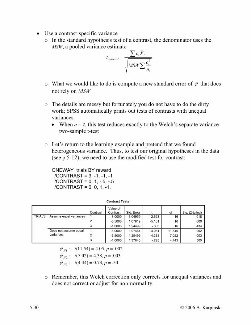
two-sample t-test o Let’s return to the learning example and pretend that we found
heterogeneous variance. Thus, to test our original hypotheses in the data (see p 5-12), we need to use the modified test for contrast:
ONEWAY trials BY reward /CONTRAST = 3, -1, -1, -1 /CONTRAST = 0, 1, -.5, -.5 /CONTRAST = 0, 0, 1, -1.
Contrast Tests
-8.0000 3.04959 -2.623 16 .018-5.5000 1.07819 -5.101 16 .000-1.0000 1.24499 -.803 16 .434-8.0000 1.97484 -4.051 11.545 .002-5.5000 1.25499 -4.383 7.022 .003-1.0000 1.37840 -.725 4.443 .505
Contrast123123
Assume equal variances
Does not assume equalvariances
TRIALS
Value ofContrast Std. Error t df Sig. (2-tailed)
:ˆ 1Hψ 002.,05.4)54.11( == pt :ˆ 2Hψ 003.,38.4)02.7( == pt :ˆ 3Hψ 50.,73.0)44.4( == pt
o Remember, this Welch correction only corrects for unequal variances and
does not correct or adjust for non-normality.

5-31 © 2006 A. Karpinski
• Try a non-parametric, rank-based alternative
o Pair-wise tests can be conducted using the Mann-Whitney U test (or an ANOVA on the ranked data).
o However, complex comparisons should be avoided! Because ranked data are ordinal data, we should not average (or take any linear combination) across groups.
o A comparison of Mann-Whitney U pairwise contrasts with ANOVA by
ranks approach 211 : µµψ = 322 : µµψ = )0,0,1,1(:1 −c )0,1,1,0(:2 −c
• Mann-Whitney U pairwise contrasts:
NPAR TESTS NPAR TESTS /M-W= trials BY reward(1 2). /M-W= trials BY reward(2 3).
Test Statistics
9.50024.500
-.638.523
.548a
Mann-Whitney UWilcoxon WZAsymp. Sig. (2-tailed)Exact Sig. [2*(1-tailedSig.)]
TRIALS
Not corrected for ties.a.
Test Statistics
.00015.000-2.652
.008
.008a
Mann-Whitney UWilcoxon WZAsymp. Sig. (2-tailed)Exact Sig. [2*(1-tailedSig.)]
TRIALS
Not corrected for ties.a.
• ANOVA by ranks approach: RANK VARIABLES=trials. ONEWAY rtrials BY reward /CONT= -1 1 0 0 /CONT= 0 1 -1 0.
Contrast Tests
-1.30000 2.391129 -.544 16 .594-8.80000 2.391129 -3.680 16 .002-1.30000 2.230471 -.583 5.397 .584
-8.80000 2.173707 -4.048 4.954 .010
Contrast1212
Assume equal variances
Does not assume equalvariances
RANK of TRIALS
Value ofContrast Std. Error t df Sig. (2-tailed)

5-32 © 2006 A. Karpinski
Approach Contrast Mann-Whitney U ANOVA by Ranks 21 µµ = z = -0.638, p = .523 t(16) = -0.544, p = .594 32 µµ = z = -2.652, p = .008 t(16) = -3.680, p = .002
o A rank modification of ANOVA is easy to use but: • Not much theoretical work has been done on this type of test. • This approach is probably not valid for multi-factor ANOVA. • This approach is likely to be trouble for complex comparisons. • Remember that the conclusions you draw are on the ranks, and not on
the observed values!
7. Effect sizes for a single contrast
• For pairwise contrasts, you can use Hedges’s g:
g =X 1 − X 2
ˆ σ =
X 1 − X 2MSW
• In the general case there are several options
o Use omega squared ( 2ω )
MSWSSTMSWSS
+−
=ψωˆˆ 2
2ω = .01 small effect size 2ω = .06 medium effect size 2ω = .15 large effect size
2ω has an easy interpretation: it is the percentage of the variance in
the dependent variable (in the population) that is accounted for by the contrast
5-33 © 2006 A. Karpinski
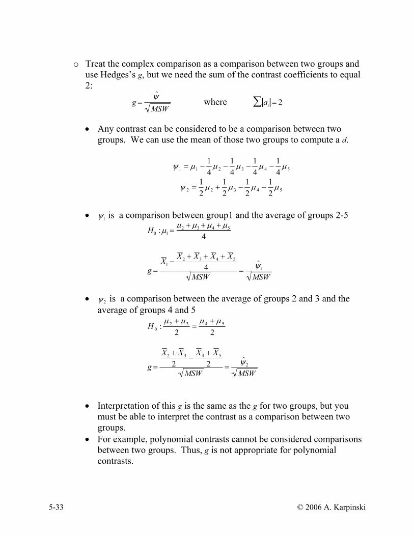
o Treat the complex comparison as a comparison between two groups and
use Hedges’s g, but we need the sum of the contrast coefficients to equal 2:
g =ˆ ψ
MSW where ai∑ = 2
• Any contrast can be considered to be a comparison between two
groups. We can use the mean of those two groups to compute a d.
543211 41
41
41
41 µµµµµψ −−−−=
54322 21
21
21
21 µµµµψ −−+=
• ψ1 is a comparison between group1 and the average of groups 2-5
H0 : µ1 =µ2 + µ3 + µ4 + µ5
4
g =X 1 −
X 2 + X 3 + X 4 + X 54
MSW=
ˆ ψ 1MSW
• ψ2 is a comparison between the average of groups 2 and 3 and the
average of groups 4 and 5
22: 5432
0µµµµ +
=+
H
g =
X 2 + X 32
−X 4 + X 5
2MSW
=ˆ ψ 2
MSW
• Interpretation of this g is the same as the g for two groups, but you must be able to interpret the contrast as a comparison between two groups.
• For example, polynomial contrasts cannot be considered comparisons between two groups. Thus, g is not appropriate for polynomial contrasts.

5-34 © 2006 A. Karpinski
o Compute an r measure of effect size:
r =Fcontrast
Fcontrast + dfwithin
=tcontrast
2
tcontrast2 + dfwithin
• r is interpretable as the (partial) correlation between the group means and the contrast values, controlling for non-contrast variability.
8. An example
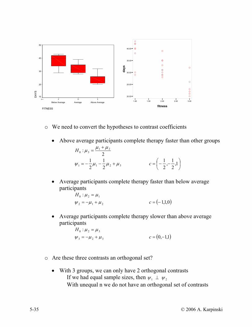
• Rehabilitation Example. We have a sample of 24 male participants between the age of 18 and 30 who have all undergone corrective knee surgery in the past year. We would like to investigate the relationship between prior physical fitness status (below average, average, above average) and the number of days required for successful completion of physical therapy.
Prior physical fitness status
Below Average
Average
Above Average
29 30 26 42 35 32 38 39 21 40 28 20 43 31 23 40 31 22 30 29 42 35 29 33
o We would like to test if:
• Above average participants complete therapy faster than other groups • Average participants complete therapy faster than below average
participants • Average participants complete therapy slower than above average
participants
5-35 © 2006 A. Karpinski
6108N =
FITNESS
Above AverageAverageBelow Average
DA
YS
50
40
30
20
10
1.00 1.50 2.00 2.50 3.00
fitness
20.00
25.00
30.00
35.00
40.00
days
A
A
A
A
A
A
A
A
A
A
A
A
AA
A
A
A
A
A
A
AA
AA
o We need to convert the hypotheses to contrast coefficients
• Above average participants complete therapy faster than other groups
2: 21
30µµ
µ+
=H
3211 21
21 µµµψ +−−=
−−= 1,
21,
21c
• Average participants complete therapy faster than below average
participants 120 : µµ =H
212 µµψ +−= ( )0,1,1−=c
• Average participants complete therapy slower than above average participants
320 : µµ =H
323 µµψ +−= ( )1,1,0 −=c
o Are these three contrasts an orthogonal set?
• With 3 groups, we can only have 2 orthogonal contrasts If we had equal sample sizes, then 1ψ ⊥ 2ψ With unequal n we do not have an orthogonal set of contrasts

5-36 © 2006 A. Karpinski
o Conduct significance tests for these contrasts
ONEWAY days BY fitness /STAT desc /CONTRAST = -.5,-.5,1 /CONTRAST = -1, 1, 0 /CONTRAST = 0, -1, 1.
Descriptives
DAYS
8 38.0000 5.47723 1.93649 33.4209 42.579110 32.0000 3.46410 1.09545 29.5219 34.4781
6 24.0000 4.42719 1.80739 19.3540 28.646024 32.0000 6.87782 1.40393 29.0958 34.9042
Below AverageAverageAbove AverageTotal
N Mean Std. Deviation Std. Error Lower Bound Upper Bound
95% Confidence Interval forMean
ANOVA
DAYS
672.000 2 336.000 16.962 .000416.000 21 19.810
1088.000 23
Between GroupsWithin GroupsTotal
Sum ofSquares df Mean Square F Sig.
Contrast Coefficients
-.5 -.5 1-1 1 00 -1 1
Contrast123
BelowAverage Average
AboveAverage
FITNESS
Contrast Tests
-11.0000 2.10140 -5.235 21 .000-6.0000 2.11119 -2.842 21 .010-8.0000 2.29838 -3.481 21 .002
-11.0000 2.12230 -5.183 8.938 .001-6.0000 2.22486 -2.697 11.297 .020-8.0000 2.11345 -3.785 8.696 .005
Contrast123123
Assume equal variances
Does not assume equalvariances
DAYS
Value ofContrast Std. Error t df Sig. (2-tailed)
5-37 © 2006 A. Karpinski
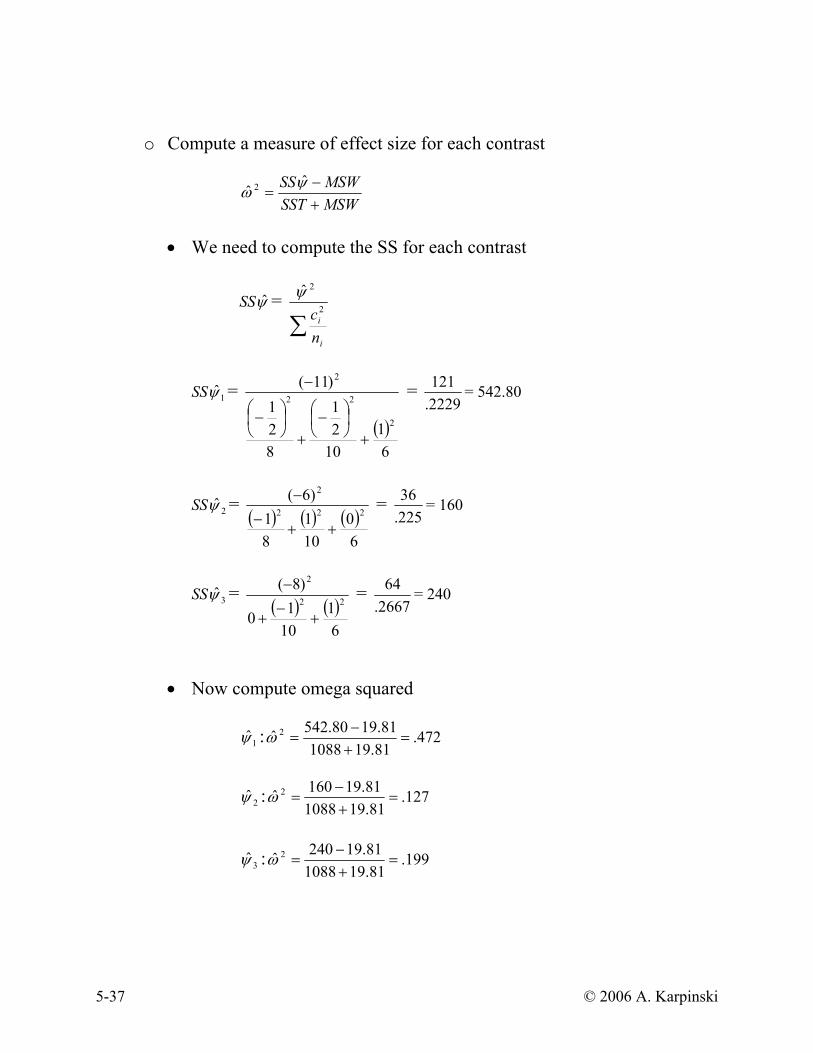
o Compute a measure of effect size for each contrast
MSWSSTMSWSS
+−
=ψωˆˆ 2
• We need to compute the SS for each contrast
SSψ̂ = ∑
i
i
nc 2
2 ψ̂
SS 1ψ̂ =
( )6
11021
821
)11(
2
22
2
+
−
+
−
− = 2229.121 = 542.80
SS 2ψ̂ = ( ) ( ) ( )
60
101
81
)6(222
2
++−
− = 225.36 = 160
SS 3ψ̂ = ( ) ( )
61
1010
)8(22
2
+−
+
− = 2667.64 = 240
• Now compute omega squared
1ψ̂ : 472.81.19108881.1980.542ˆ 2 =
+−
=ω
2ψ̂ : 127.81.19108881.19160ˆ 2 =
+−
=ω
3ψ̂ : 199.81.19108881.19240ˆ 2 =
+−
=ω

5-38 © 2006 A. Karpinski
• OR Compute an r measure of effect size for each contrast:
r =Fcontrast
Fcontrast + dfwithin
=tcontrast
2
tcontrast2 + dfwithin
1ψ̂ : r1 =5.2352
5.2352 + 21= .75
2ψ̂ : r2 =2.8422
2.8422 + 21= .53
3ψ̂ : r2 =3.4812
3.4812 + 21= .61
o Report the results
1ψ̂ : 47.,01.,24.5)21( 2 =<−= ωpt
2ψ̂ : 13.,01.,84.2)21( 2 ==−= ωpt
3ψ̂ : 20.,01.,48.3)21( 2 =<−= ωpt
• In your results section, you need to say in English (not in statistics or symbols) what each contrast is testing
• In general, it is not necessary to report the value of the contrast or the contrast coefficients used
. . . A contrast revealed that above average individuals recovered faster than all other individuals, 47.,01.,24.5)21( 2 =<−= ωpt . Pairwise tests also revealed that average individuals completed therapy faster than below average individuals, 13.,01.,84.2)21( 2 ==−= ωpt , and that above average individuals completed therapy faster than average participants,
20.,01.,48.3)21( 2 =<−= ωpt .

5-39 © 2006 A. Karpinski
9. Polynomial Trend Contrasts
• Trend contrasts are a specific kind of orthogonal contrasts that may be of interest for certain designs.
• Tests for trends are used only for comparing quantitative (ordered) independent variables. o IV = 10mg, 20mg, 30mg, 40mg of a drug
• Trend contrasts are used to explore polynomial trends in the data
Order of # of Trend Polynomial Bends Shape Linear 1st 0 Straight Line Quadratic 2nd 1 U-shaped Cubic 3rd 2 Wave Quartic 4th 3 Wave Etc.
Linear
-3-2-10123
1 2 3 4 5
Quadratic
-3-2-10123
1 2 3 4 5
Cubic
-3-2-10123
1 2 3 4 5
Quartic
-5
0
5
10
1 2 3 4 5
5-40 © 2006 A. Karpinski
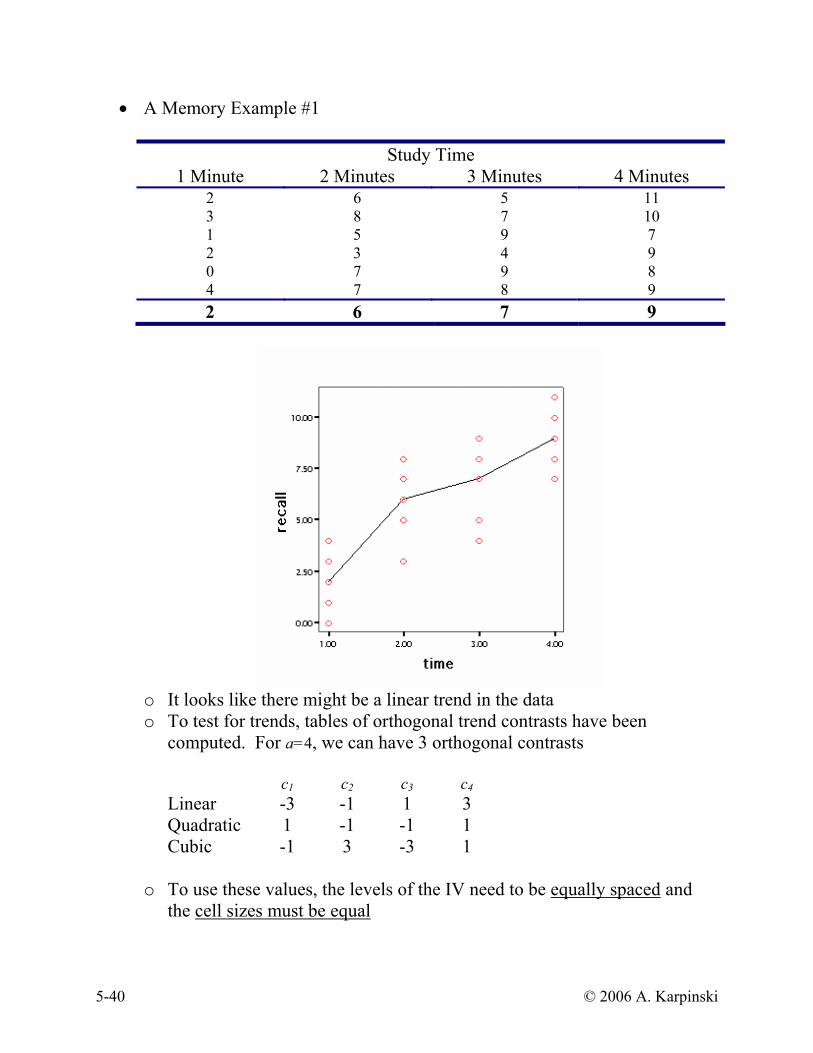
• A Memory Example #1
Study Time 1 Minute 2 Minutes 3 Minutes 4 Minutes
2 6 5 11 3 8 7 10 1 5 9 7 2 3 4 9 0 7 9 8 4 7 8 9 2 6 7 9
o It looks like there might be a linear trend in the data o To test for trends, tables of orthogonal trend contrasts have been
computed. For a=4, we can have 3 orthogonal contrasts c1 c2 c3 c4 Linear -3 -1 1 3 Quadratic 1 -1 -1 1 Cubic -1 3 -3 1
o To use these values, the levels of the IV need to be equally spaced and the cell sizes must be equal
5-41 © 2006 A. Karpinski
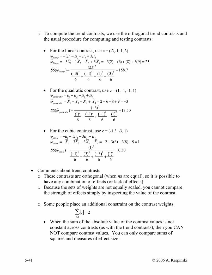
o To compute the trend contrasts, we use the orthogonal trend contrasts and
the usual procedure for computing and testing contrasts:
• For the linear contrast, use c = (-3,-1, 1, 3) ψ linear = −3µ1 − µ2 + µ3 + 3µ4 ˆ ψ linear = −3X 1 −1X 2 + X 3 + 3X 4 = −3(2) − (6) + (8) + 3(9) = 23
SS( ˆ ψ linear ) =(23)2
(−3)2
6+
(−1)2
6+
1( )2
6+
3( )2
6
=158.7
• For the quadratic contrast, use c = (1, -1, -1, 1)
ψquadratic = µ1 −µ2 −µ3 + µ4 ˆ ψ quadratic = X 1 − X 2 − X 3 + X 4 = 2 − 6 −8 + 9 = −3
SS( ˆ ψ quadratic) =(−3)2
(1)2
6+
(−1)2
6+
−1( )2
6+
1( )2
6
=13.50
• For the cubic contrast, use c = (-1,3, -3, 1)
ψcubic = −µ1 + 3µ2 − 3µ3 + µ4 ˆ ψ cubic = −X 1 + 3X 2 − 3X 3 + X 4 = −2 + 3(6) − 3(8) + 9 =1
SS( ˆ ψ cubic) =(1)2
(−1)2
6+
(3)2
6+
−3( )2
6+
1( )2
6
= 0.30
• Comments about trend contrasts
o These contrasts are orthogonal (when ns are equal), so it is possible to have any combination of effects (or lack of effects)
o Because the sets of weights are not equally scaled, you cannot compare the strength of effects simply by inspecting the value of the contrast.
o Some people place an additional constraint on the contrast weights:
cii=1
a
∑ = 2
• When the sum of the absolute value of the contrast values is not constant across contrasts (as with the trend contrasts), then you CAN NOT compare contrast values. You can only compare sums of squares and measures of effect size.

5-42 © 2006 A. Karpinski
• A Memory Example #2
Study Time 1 Minute 2 Minutes 3 Minutes 4 Minutes
6 6 5 14 7 8 7 13 5 5 9 10 6 3 4 12 4 7 9 11 8 7 8 12
6 6 7 12
o Looks like we have a linear effect with some quadratic
ψ linear = −3µ1 − µ2 + µ3 + 3µ4 ˆ ψ linear = −3X 1 −1X 2 + X 3 + 3X 4 = −3(6) − (6) + (7) + 3(12) =19
SS( ˆ ψ linear ) =(19)2
(−3)2
6+
(−1)2
6+
1( )2
6+
3( )2
6
=108.3
ψquadratic = µ1 −µ2 −µ3 + µ4 ˆ ψ quadratic = X 1 − X 2 − X 3 + X 4 = 6 − 6 − 7 +12 = 5
SS( ˆ ψ quadratic) =(5)2
(1)2
6+
(−1)2
6+
−1( )2
6+
1( )2
6
= 37.50
ψcubic = −µ1 + 3µ2 − 3µ3 + µ4 ˆ ψ cubic = −X 1 + 3X 2 − 3X 3 + X 4 = −6 + 3(6) − 3(7) +12 = 3
SS( ˆ ψ cubic) =(3)2
(−1)2
6+
(3)2
6+
−3( )2
6+
1( )2
6
= 2.70

5-43 © 2006 A. Karpinski
• A Memory Example #3 Study Time
1 Minute 2 Minutes 3 Minutes 4 Minutes 11 6 5 14 12 8 7 13 10 5 9 10 11 3 4 12 10 7 9 11 12 7 8 12
11 6 7 12
• Looks like we have a quadratic effect
ψ linear = −3µ1 − µ2 + µ3 + 3µ4 ˆ ψ linear = −3X 1 −1X 2 + X 3 + 3X 4 = −3(11) − (6) + (7) + 3(12) = 4
SS( ˆ ψ linear ) =(4)2
(−3)2
6+
(−1)2
6+
1( )2
6+
3( )2
6
= 4.8
ψquadratic = µ1 −µ2 −µ3 + µ4 ˆ ψ quadratic = X 1 − X 2 − X 3 + X 4 = 6 − 6 − 7 +12 =10
SS( ˆ ψ quadratic) =(10)2
(1)2
6+
(−1)2
6+
−1( )2
6+
1( )2
6
=150
ψcubic = −µ1 + 3µ2 − 3µ3 + µ4 ˆ ψ cubic = −X 1 + 3X 2 − 3X 3 + X 4 = −11+ 3(6) − 3(7) +12 = −2
SS( ˆ ψ cubic) =(−2)2
(−1)2
6+
(3)2
6+
−3( )2
6+
1( )2
6
=1.20

5-44 © 2006 A. Karpinski
• Statistical tests for trend analysis: Reanalyzing the learning example
o Our learning example is perfectly suited for a trend analysis (Why?) o When we initially analyzed these data, we selected one set of orthogonal
contrasts, but there are many possible sets of orthogonal contrasts, including the trend contrasts
1.00 2.00 3.00 4.00
reward
10.00
12.50
15.00
17.50
20.00
tria
ls
A
A
A
AA
A
A
A
A
A
A
A
A
AA
A
A
A
A
A
A
A
A
A
o For a = 4, we can test for a linear, a quadratic, and a cubic trend
c1 c2 c3 c4 Linear -3 -1 1 3 Quadratic 1 -1 -1 1 Cubic -1 3 -3 1
20 )17(3)16()11()12(3
33ˆ 4321
=++−−=
++−−= XXXXlinearψ
2 )17()16()11()12(
ˆ 4321
=+−−=
+−−= XXXXquadraticψ
SS( ˆ ψ lin ) =(20)2
(−3)2
5+
(−1)2
5+
1( )2
5+
3( )2
5
=100 SS( ˆ ψ quad ) =(2)2
(1)2
5+
(−1)2
5+
−1( )2
5+
1( )2
5
= 5
10 )17()16(3)11(3)12(
33ˆ 4321
−=+−+−=
+−+−= XXXXcubicψ
SS( ˆ ψ cubic) =(−10)2
(−1)2
5+
(3)2
5+
−3( )2
5+
1( )2
5
= 25

5-45 © 2006 A. Karpinski
o Rather than determine significance by hand, we can use ONEWAY:
ONEWAY trials BY reward /CONT -3, -1, 1, 3 /CONT 1, -1, -1, 1 /CONT -1, 3, -3, 1.
Contrast Coefficients
-3 -1 1 31 -1 -1 1
-1 3 -3 1
Contrast123
1.00 2.00 3.00 4.00REWARD
Contrast Tests
20.0000 3.93700 5.080 16 .0002.0000 1.76068 1.136 16 .273
-10.0000 3.93700 -2.540 16 .022
Contrast123
Assume equal variancesTRIALS
Value ofContrast Std. Error t df Sig. (2-tailed)
• We find evidence for significant linear and cubic trends
79.,01.,08.5)16(:ˆ =<= rptlinearψ
27.,27.,14.1)16(:ˆ === rptquadraticψ
54.,02.,54.2)16(:ˆ ==−= rptcubicψ

5-46 © 2006 A. Karpinski
• To complete the ANOVA table, we need the sums of squares for each
contrast
SSψ̂ = ∑
i
i
nc 2
2 ψ̂
SS ˆ ψ linear =100 SS ˆ ψ quad = 5 SS ˆ ψ cubic = 25
SS linearψ̂ + SS quadraticψ̂ + SS cubicψ̂ = 100 + 5 + 25 = 130 = SSB
ANOVA Source of Variation SS df MS F P-value
Between Groups 130 3 43.33333 11.1828 0.000333 linψ̂ 100 1 100 25.806 0.000111 quadψ̂ 5 1 5 1.290 0.272775 cubicψ̂ 25 1 25 6.452 0.021837 Within Groups 62 16 3.875 Total 192 19

5-47 © 2006 A. Karpinski
• You can also directly ask for polynomial contrasts in SPSS
o Method 1: ONEWAY
ONEWAY trials BY reward /POLYNOMIAL= 3.
• After polynomial, enter the highest degree polynomial you wish to
test.
ANOVA
TRIALS
130.000 3 43.333 11.183 .000100.000 1 100.000 25.806 .000
30.000 2 15.000 3.871 .043
5.000 1 5.000 1.290 .27325.000 1 25.000 6.452 .02225.000 1 25.000 6.452 .02262.000 16 3.875
192.000 19
(Combined)ContrastDeviation
Linear Term
ContrastDeviation
QuadraticTerm
ContrastCubic Term
BetweenGroups
Within GroupsTotal
Sum ofSquares df Mean Square F Sig.
o Advantages of the ONEWAY method for polynomial contrasts:
• It utilizes the easiest oneway ANOVA command • It gives you the sums of squares of the contrast • It uses the spacing of the IV in the data (Be careful!) • It gives you the “deviation” test (to be explained later)
o Disadvantages of the ONEWAY method for polynomial contrasts:
• You can not see the value of the contrast or the contrast coefficients

5-48 © 2006 A. Karpinski
o Method 2: UNIANOVA
UNIANOVA trials BY reward /CONTRAST (reward)=Polynomial /PRINT = test(lmatrix).
Contrast Results (K Matrix)
4.4720
4.472
.880
.0002.6066.3381.000
0
1.000
.880
.273-.8662.866
-2.2360
-2.236
.880
.022-4.102
-.370
Contrast EstimateHypothesized ValueDifference (Estimate - Hypothesized)
Std. ErrorSig.
Lower BoundUpper Bound
95% Confidence Intervalfor Difference
Contrast EstimateHypothesized ValueDifference (Estimate - Hypothesized)
Std. ErrorSig.
Lower BoundUpper Bound
95% Confidence Intervalfor Difference
Contrast EstimateHypothesized ValueDifference (Estimate - Hypothesized)
Std. ErrorSig.
Lower BoundUpper Bound
95% Confidence Intervalfor Difference
REWARDPolynomial Contrasta
Linear
Quadratic
Cubic
TRIALS
DependentVariable
Metric = 1.000, 2.000, 3.000, 4.000a.
Test Results
Dependent Variable: TRIALS
130.000 3 43.333 11.183 .00062.000 16 3.875
SourceContrastError
Sum ofSquares df Mean Square F Sig.

5-49 © 2006 A. Karpinski
Contrast Coefficients (L' Matrix)
.000 .000 .000-.671 .500 -.224-.224 -.500 .671.224 -.500 -.671.671 .500 .224
ParameterIntercept[REWARD=1.00][REWARD=2.00][REWARD=3.00][REWARD=4.00]
Linear Quadratic Cubic
REWARD Polynomial Contrasta
The default display of this matrix is the transpose of thecorresponding L matrix.
Metric = 1.000, 2.000, 3.000, 4.000a.
• This is the matrix of trend coefficients used by SPSS to calculate the contrasts. SPSS coefficients SPSS coefficients X 6
)671,.224,.224.,671.(1 −−=c )4,1,1,4(1 −−=c ( )5,.5.,5.,5.2 −−=c ( )3,3,3,32 −−=c ( )224.671.,671,.224.3 −−=c ( )1,4,4,13 −−=c
• You can check that these coefficients are orthogonal
o Suppose the reward intervals were not equally spaced:
Level of Reward Constant (100%)
Frequent (75%)
Infrequent (25%)
Never (0%)
• Now we cannot use the tabled contrast values, because they require
equal spacing between intervals

5-50 © 2006 A. Karpinski
Equal spacing Unequal spacing
1.00 2.00 3.00 4.00
reward
10.00
12.50
15.00
17.50
20.00
tria
ls
A
A
A
AA
A
A
A
A
A
A
A
A
AA
A
A
A
A
A
A
A
A
A
0.00 0.25 0.50 0.75 1.00
reward2
10.00
12.50
15.00
17.50
20.00
tria
ls
A
A
A
AA
A
A
A
A
A
A
A
A
AA
A
A
A
A
A
A
A
A
A
UNIANOVA trials BY reward /CONTRAST (reward)=Polynomial (1, .75, .25, 0) /PRINT = test(lmatrix).
Contrast Results (K Matrix)
-4.7430
-4.743
.880
.000-6.610-2.8771.000
0
1.000
.880
.273-.8662.8661.581
0
1.581
.880
.091-.2853.447
Contrast EstimateHypothesized ValueDifference (Estimate - Hypothesized)
Std. ErrorSig.
Lower BoundUpper Bound
95% Confidence Intervalfor Difference
Contrast EstimateHypothesized ValueDifference (Estimate - Hypothesized)
Std. ErrorSig.
Lower BoundUpper Bound
95% Confidence Intervalfor Difference
Contrast EstimateHypothesized ValueDifference (Estimate - Hypothesized)
Std. ErrorSig.
Lower BoundUpper Bound
95% Confidence Intervalfor Difference
REWARDPolynomial Contrasta
Linear
Quadratic
Cubic
TRIALS
DependentVariable
Metric = 1.000, .750, .250, .000a.

5-51 © 2006 A. Karpinski
• Now only the linear trend is significant
• SPSS calculates a set of orthogonal trend contrasts, based on the
spacing you provide. Here they are:
Contrast Coefficients (L' Matrix)
.000 .000 .000
.632 .500 .316
.316 -.500 -.632-.316 -.500 .632-.632 .500 -.316
ParameterIntercept[REWARD=1.00][REWARD=2.00][REWARD=3.00][REWARD=4.00]
Linear Quadratic Cubic
REWARD Polynomial Contrasta
The default display of this matrix is the transpose of thecorresponding L matrix.
Metric = 1.000, .750, .250, .000a.
o Advantages of the UNIANOVA method:
• It is the only way SPSS gives you confidence intervals for a contrast (But remember, the width of CIs depends on the contrast values)
• It allows you to deal with unequally spaced intervals (It assumes equal spacing unless you tell it otherwise; no matter how you have the data coded!)
• It will print the contrast values SPSS uses
o Disadvantages of the UNIANOVA method: • It does not print out a test statistic or the degrees of freedom of the
test!?!
• Remember, for a one-way design, you can obtain a test of any contrast by using the ONEWAY command and entering the values for each contrast. With ONEWAY method, you know exactly how the contrast is being computed and analyzed
5-52 © 2006 A. Karpinski
10. Simultaneous significance tests on multiple orthogonal contrasts
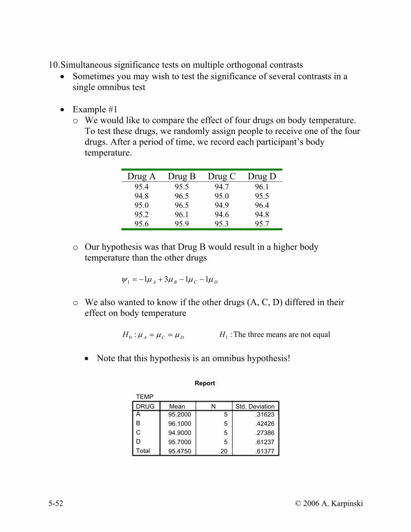
• Sometimes you may wish to test the significance of several contrasts in a single omnibus test
• Example #1
o We would like to compare the effect of four drugs on body temperature. To test these drugs, we randomly assign people to receive one of the four drugs. After a period of time, we record each participant’s body temperature.
Drug A Drug B Drug C Drug D
95.4 95.5 94.7 96.1 94.8 96.5 95.0 95.5 95.0 96.5 94.9 96.4 95.2 96.1 94.6 94.8 95.6 95.9 95.3 95.7
o Our hypothesis was that Drug B would result in a higher body
temperature than the other drugs
DCBA µµµµψ 11311 −−+−=
o We also wanted to know if the other drugs (A, C, D) differed in their effect on body temperature
DCAH µµµ ==:0 :1H The three means are not equal
• Note that this hypothesis is an omnibus hypothesis!
Report
TEMP
95.2000 5 .3162396.1000 5 .4242694.9000 5 .2738695.7000 5 .6123795.4750 20 .61377
DRUGABCDTotal
Mean N Std. Deviation

5-53 © 2006 A. Karpinski
o Step 1: Obtain SSB, SST, and MSW ANOVA
TEMP
4.237 3 1.412 7.740 .0022.920 16 .1837.157 19
Between GroupsWithin GroupsTotal
Sum ofSquares df Mean Square F Sig.
o Step 2: Test DCBA µµµµψ 11311 −−+−=
5.2)5.97(1)9.94(1)1.96(3)2.95(1ˆ1 =−−+−=ψ
SS 1ψ̂ = ( ) ( ) ( ) ( )
51
51
53
51
)5.2(2222
2
−+
−++
− =
4.225.6 = 2.6042
ANOVA
Source of Variation SS df MS F P-value Between Groups 4.237 3 1.412 7.740 .002 1ψ 2.6042 1 2.6042 14.2694 0.0017 Within Groups 2.92 16 .1825 Total 7.1575 19
o Step 3: Test DCAH µµµ ==:0 • The trick is to remember that an omnibus ANOVA test m means is
equal to the simultaneous test on any set of (m-1) orthogonal contrasts • We can then combine these orthogonal contrasts in a single omnibus
F-test:
Fcomb (m −1,dfw) =
SSC1 + ...+ SSCm −1
m −1MSW
5-54 © 2006 A. Karpinski
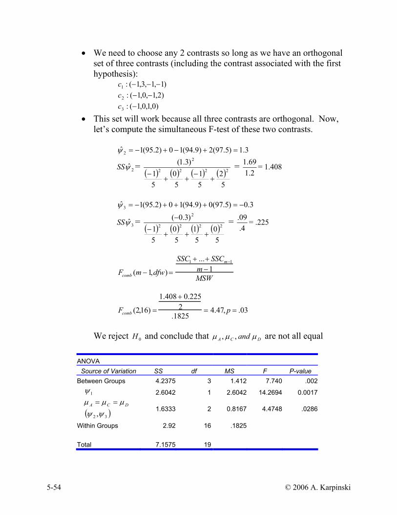
• We need to choose any 2 contrasts so long as we have an orthogonal set of three contrasts (including the contrast associated with the first hypothesis):
)1,1,3,1(:1 −−−c )2,1,0,1(:2 −−c
)0,1,0,1(:3 −c • This set will work because all three contrasts are orthogonal. Now,
let’s compute the simultaneous F-test of these two contrasts.
3.1)5.97(2)9.94(10)2.95(1ˆ 2 =+−+−=ψ
SS 2ψ̂ = ( ) ( ) ( ) ( )
52
51
50
51
)3.1(2222
2
+−
++−
= 2.169.1 = 1.408
3.0)5.97(0)9.94(10)2.95(1ˆ 3 −=+++−=ψ
SS 3ψ̂ = ( ) ( ) ( ) ( )
50
51
50
51
)3.0(2222
2
+++−
− = 4.09. = .225
Fcomb (m −1,dfw) =
SSC1 + ...+ SSCm −1
m −1MSW
Fcomb (2,16) =
1.408 + 0.2252
.1825= 4.47, p = .03
We reject 0H and conclude that DCA and µµµ , , are not all equal
ANOVA
Source of Variation SS df MS F P-value Between Groups 4.2375 3 1.412 7.740 .002 1ψ 2.6042 1 2.6042 14.2694 0.0017 DCA µµµ == ( )32 ,ψψ
1.6333 2 0.8167 4.4748
.0286
Within Groups 2.92 16 .1825 Total 7.1575 19

5-55 © 2006 A. Karpinski
o Note: We also could have computed the test of µA = µC = µD without directly computing the two orthogonal contrasts: • If we knew the combined sums of squares of these two contrasts then
we could fill in the remainder of the ANOVA table. • But we do know the combined sums of squares for the remaining two
contrasts (so long as all the contrasts are orthogonal)!
ANOVA Source of Variation SS df MS F P-value
Between Groups 4.2375 3 1.412 7.740 .002 1ψ 2.6042 1 2.6042 14.2694 0.0017 DCA µµµ ==
2
Within Groups 2.92 16 .1825 Total 7.1575 19
321 ψψψ SSSSSSSSB ++= 6333.16042.22375.4132 =−=−=+ ψψψ SSSSBSSSS
• We can substitute SSψ2 + SSψ3 into the table and compute the F-test as we did previous (except in this case, we never identified or computed the two additional contrasts to complete the orthogonal set).
ANOVA Source of Variation SS df MS F P-value
Between Groups 4.2375 3 1.412 7.740 .002 1ψ 2.6042 1 2.6042 14.2694 0.0017 DCA µµµ ==
1.6333 2 0.8167 4.4748
.0286
Within Groups 2.92 16 .1825 Total 7.1575 19

5-56 © 2006 A. Karpinski
• Example #2
o We want to examine the effect of caffeine on cognitive performance and attention. Participants are randomly assigned to one of 5 dosages of caffeine. In a subsequent proofreading task, we count the number of errors.
Dose of Caffeine
0mg 50mg 100mg 150mg 200mg 2 2 0 1 2 4 3 1 0 3 5 4 3 2 4 3 2 1 1 4 2 2 1 1 2 1 1 2 2 1 3 2 2 1 2 3 2 1 0 3 2 3 1 1 2 4 4 2 3 2
1010101010N =
DOSE
200 mg150 mg100 mg50 mg0 mg
6
5
4
3
2
1
0
-1
5-57 © 2006 A. Karpinski
Descriptives
ERRORS
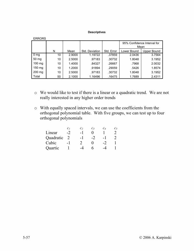
10 2.9000 1.19722 .37859 2.0436 3.756410 2.5000 .97183 .30732 1.8048 3.195210 1.4000 .84327 .26667 .7968 2.003210 1.2000 .91894 .29059 .5426 1.857410 2.5000 .97183 .30732 1.8048 3.195250 2.1000 1.16496 .16475 1.7689 2.4311
0 mg50 mg100 mg150 mg200 mgTotal
N Mean Std. Deviation Std. Error Lower Bound Upper Bound
95% Confidence Interval forMean
o We would like to test if there is a linear or a quadratic trend. We are not
really interested in any higher order trends
o With equally spaced intervals, we can use the coefficients from the orthogonal polynomial table. With five groups, we can test up to four orthogonal polynomials
c1 c2 c3 c4 c5 Linear -2 -1 0 1 2 Quadratic 2 -1 -2 -1 2 Cubic -1 2 0 -2 1 Quartic 1 -4 6 -4 1

5-58 © 2006 A. Karpinski
o Method 1: Let SPSS do all the work
ONEWAY errors BY dose /POLYNOMIAL= 2.
ANOVA
ERRORS
22.600 4 5.650 5.792 .0014.410 1 4.410 4.521 .039
18.190 3 6.063 6.215 .001
13.207 1 13.207 13.538 .0014.983 2 2.491 2.554 .089
43.900 45 .97666.500 49
(Combined)ContrastDeviation
Linear Term
ContrastDeviation
QuadraticTerm
BetweenGroups
Within GroupsTotal
Sum ofSquares df Mean Square F Sig.
• Under “Linear Term” CONTRAST is the test for the linear contrast: F(1,45) = 4.52, p = .039 DEVIATION is the combined test for the quadratic, cubic, and
quartic contrasts: F(3,45) = 6.62, p = .001
• Under “Quadratic Term” CONTRAST is the test for the quadratic contrast:
F(1,45) = 13.54, p = .001 DEVIATION is the combined test for the cubic and quartic contrasts
F(2,45) = 2.55, p = .089
• Is it safe to report that there are no higher order trends?

5-59 © 2006 A. Karpinski
o Method 2a: Let SPSS do some of the work ONEWAY errors BY dose /CONT= -2 -1 0 1 2 /CONT= 2 -1 -2 -1 2 /CONT= -1 2 0 -2 1 /CONT= 1 -4 6 -4 1.
Contrast Tests
-2.1000 .98770 -2.126 45 .0394.3000 1.16866 3.679 45 .0012.2000 .98770 2.227 45 .031
-1.0000 2.61321 -.383 45 .704-2.1000 1.06301 -1.976 23.575 .0604.3000 1.18930 3.616 31.679 .0012.2000 .97639 2.253 28.573 .032
-1.0000 2.37908 -.420 26.966 .678
Contrast12341234
Assume equal variances
Does not assume equalvariances
ERRORS
Value ofContrast Std. Error t df Sig. (2-tailed)
o Method 2b: Let SPSS do some of the work
UNIANOVA errors BY dose /CONTRAST (dose)=POLYNOMIAL /PRINT=TEST(LMATRIX).
Contrast Coefficients (L' Matrix)
.000 .000 .000 .000-.632 .535 -.316 .120-.316 -.267 .632 -.478.000 -.535 .000 .717.316 -.267 -.632 -.478.632 .535 .316 .120
ParameterIntercept[DOSE=1.00][DOSE=2.00][DOSE=3.00][DOSE=4.00][DOSE=5.00]
Linear Quadratic Cubic Order 4
DOSE Polynomial Contrasta
The default display of this matrix is the transpose of thecorresponding L matrix.
Metric = 1.000, 2.000, 3.000, 4.000, 5.000a.
5-60 © 2006 A. Karpinski
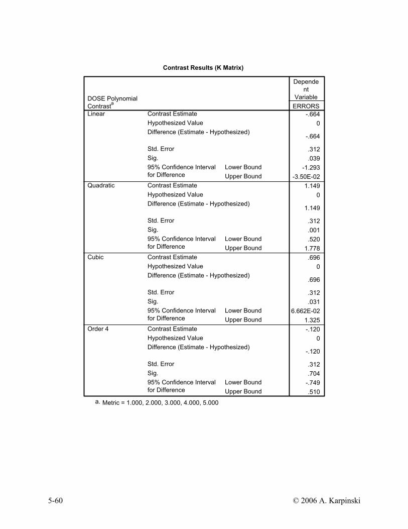
Contrast Results (K Matrix)
-.6640
-.664
.312
.039-1.293
-3.50E-021.149
0
1.149
.312
.001
.5201.778
.6960
.696
.312
.0316.662E-02
1.325-.120
0
-.120
.312
.704-.749.510
Contrast EstimateHypothesized ValueDifference (Estimate - Hypothesized)
Std. ErrorSig.
Lower BoundUpper Bound
95% Confidence Intervalfor Difference
Contrast EstimateHypothesized ValueDifference (Estimate - Hypothesized)
Std. ErrorSig.
Lower BoundUpper Bound
95% Confidence Intervalfor Difference
Contrast EstimateHypothesized ValueDifference (Estimate - Hypothesized)
Std. ErrorSig.
Lower BoundUpper Bound
95% Confidence Intervalfor Difference
Contrast EstimateHypothesized ValueDifference (Estimate - Hypothesized)
Std. ErrorSig.
Lower BoundUpper Bound
95% Confidence Intervalfor Difference
DOSE PolynomialContrasta
Linear
Quadratic
Cubic
Order 4
ERRORS
Dependent
Variable
Metric = 1.000, 2.000, 3.000, 4.000, 5.000a.
5-61 © 2006 A. Karpinski
o Here are the results
30.,039.,13.2)45(:ˆ ==−= rptlinearψ 48.,001.,68.3)45(:ˆ === rptquadraticψ
32.,031.,23.2)45(:ˆ === rptcubicψ 06.,704.,38.0)45(:ˆ ==−= rptquarticψ
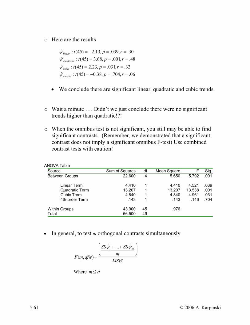
• We conclude there are significant linear, quadratic and cubic trends.
o Wait a minute . . . Didn’t we just conclude there were no significant trends higher than quadratic!?!
o When the omnibus test is not significant, you still may be able to find
significant contrasts. (Remember, we demonstrated that a significant contrast does not imply a significant omnibus F-test) Use combined contrast tests with caution!
ANOVA Table
Source Sum of Squares df Mean Square F Sig.Between Groups 22.600 4 5.650 5.792 .001
Linear Term 4.410 1
4.410
4.521 .039
Quadratic Term 13.207 1 13.207 13.538 .001Cubic Term 4.840 1 4.840 4.961 .0314th-order Term
.143 1 .143 .146 .704
Within Groups 43.900 45 .976 Total 66.500 49
• In general, to test m orthogonal contrasts simultaneously
F(m,dfw) =
SS ˆ ψ 1 + ...+ SS ˆ ψ mm
MSW
Where m ≤ a
5-62 © 2006 A. Karpinski
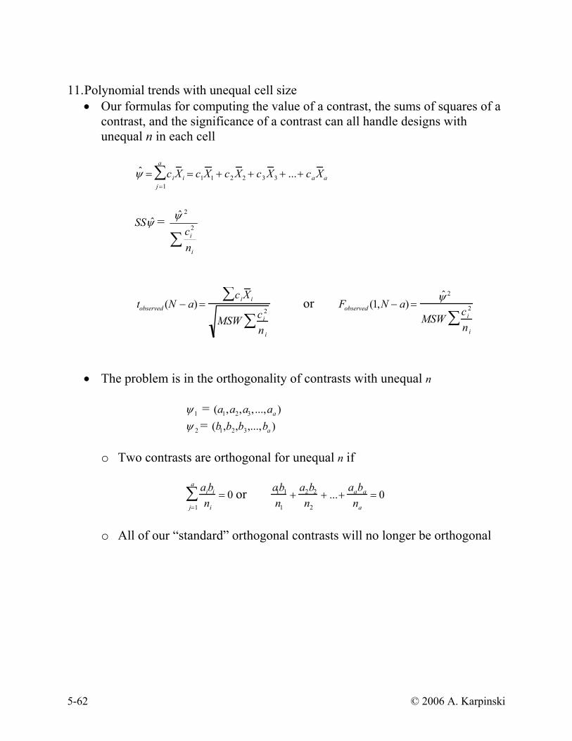
11. Polynomial trends with unequal cell size
• Our formulas for computing the value of a contrast, the sums of squares of a contrast, and the significance of a contrast can all handle designs with unequal n in each cell
ˆ ψ = ciX i = c1X 1
j =1
a
∑ + c2 X 2 + c3 X 3 + ...+ ca X a
SSψ̂ = ∑
i
i
nc 2
2 ψ̂
tobserved (N − a) =ciX i∑
MSW ci2
ni∑
or Fobserved (1,N − a) =ˆ ψ 2
MSWci
2
ni∑
• The problem is in the orthogonality of contrasts with unequal n
1ψ = (a1,a2,a3, ...,aa ) 2ψ = (b1,b2,b3,...,ba )
o Two contrasts are orthogonal for unequal n if
aibi
nij=1
a
∑ = 0 or a1b1
n1
+a2b2
n2
+ ...+aaba
na
= 0
o All of our “standard” orthogonal contrasts will no longer be orthogonal

5-63 © 2006 A. Karpinski
• Example #1 with unequal n
It was of interest to determine the effects of the ingestion of alcohol on anxiety level. Five groups of 50 year-old adults were administered between 0 and 4 ounces of pure alcohol per day over a one-month period. At the end of the experiment, their anxiety scores were measured with a well-known Anxiety scale.
0oz. 1oz. 2oz. 3oz. 4oz. 115 99 91 84 99 133 92 103 83 93 110 103 109 87 87 125 105 98 95 88 120 100 64 112 93 106
jX 120.75 103.80 100.00 82.60 95.80
jn 4 5 7 5 5
55754N =
ALCOHOL
4.003.002.001.00.00
AN
XIE
TY
140
120
100
80
60
40
21
20
9
0.00 1.00 2.00 3.00 4.00
alcohol
70.00
90.00
110.00
130.00
anxi
ety
A
A
A
A
A
A
AA
A
A
A
A
AA
A
A
AA
A
A
A
A
A
AA
A
A
AA
A
A

5-64 © 2006 A. Karpinski
o We would like to test for linear, quadratic, cubic and higher-order trends
UNIANOVA anxiety BY alcohol /CONTRAST (alcohol)=Polynomial /PRINT=test(LMATRIX) .
Contrast Coefficients (L' Matrix)
.000 .000 .000 .000-.632 .535 -.316 .120-.316 -.267 .632 -.478.000 -.535 .000 .717.316 -.267 -.632 -.478.632 .535 .316 .120
ParameterIntercept[ALCOHOL=.00][ALCOHOL=1.00][ALCOHOL=2.00][ALCOHOL=3.00][ALCOHOL=4.00]
Linear Quadratic Cubic Order 4
ALCOHOL Polynomial Contrasta
The default display of this matrix is the transpose of the correspondingL matrix.
Metric = 1.000, 2.000, 3.000, 4.000, 5.000a.
• We could also use ONEWAY, but then we could not see the contrast
coefficients
• SPSS generates these contrasts, let’s check to see if they are orthogonal
aibi
nij=1
a
∑ = 0
:Quadratic Linear vs.
( )( ) ( )( ) ( )( ) ( )( ) 05
535.632.5
267.316.05
267.316.4
535.632.≠+
−++
−−+
−
The SPSS generated contrasts are not orthogonal when ns are unequal!
• Let’s see what happens when we proceed:
SSψ̂ = ∑
i
i
nc 2
2 ψ̂

5-65 © 2006 A. Karpinski
( ) ( ) ( ) ( )484.22
80.95632.60.82316.080.103316.75.120632. 632.316.0316.632.ˆ 54321
−=+++−−=
+++−−= XXXXXlinearψ
481.12ˆ =quadψ 518.5ˆ =cubicψ 480.8ˆ =quarticψ
SS linearψ̂ = ( )( ) ( ) ( ) ( ) ( )
82.2297
5632.
5316.
70
5316.
4632.
2.484222222
2
≈+++
−+
−
SS quadraticψ̂ = ( )( ) ( ) ( ) ( ) ( )
92.786
5632.
5316.
70
5316.
4632.
2.481122222
2
≈+++
−+
−
SS cubicψ̂ = ( )( ) ( ) ( ) ( ) ( )
54.148
5316.
5632.
70
5632.
4316.
518.522222
2
≈+
−+++
−
SS quarticψ̂ = ( )( ) ( ) ( ) ( ) ( )
74.419
5120.
5478.
7717.
5478.
4120.
48.822222
2
≈+
−++
−+
ANOVA
ANXIETY
3395.065 4 848.766 9.171 .0001943.550 21 92.5505338.615 25
Between GroupsWithin GroupsTotal
Sum ofSquares df Mean Square F Sig.

5-66 © 2006 A. Karpinski
SS linearψ̂ + SS quadraticψ̂ + SS cubicψ̂ + SS quarticψ̂ SSB = 3395.07
= 2297.82 + 786.92 + 148.54 + 419.74 = 3653.02
07.339505.3653 ≠
• For non-orthogonal contrasts, we can no longer decompose the sums
of squares additively
• One “fix” is to weight the cell means by their cell size. Using this weighted approach is equivalent to adjusting the contrast coefficients by the cell size.
• Example #2 with unequal n
Group 1 2 3 4 jX 2 4 4 2
jn 30 30 5 5
553030N =
GROUP
4.003.002.001.00
DV
8
6
4
2
0
-21.00 2.00 3.00 4.00
group
0.00
2.00
4.00
6.00
dv
A
A
A
AA
A
A
A
A
A
A
A
A
A
A
A
AA
A
A
A
AAA
A
A
A
A
A
AA
A
A
AA
A
AA
A
A
A
A
A
A
A
A
A
A
A
A
A
A
A
AA
A
A
A
A
A
A
A
AA
A
A
A
A
A
A
A
AA
A
5-67 © 2006 A. Karpinski
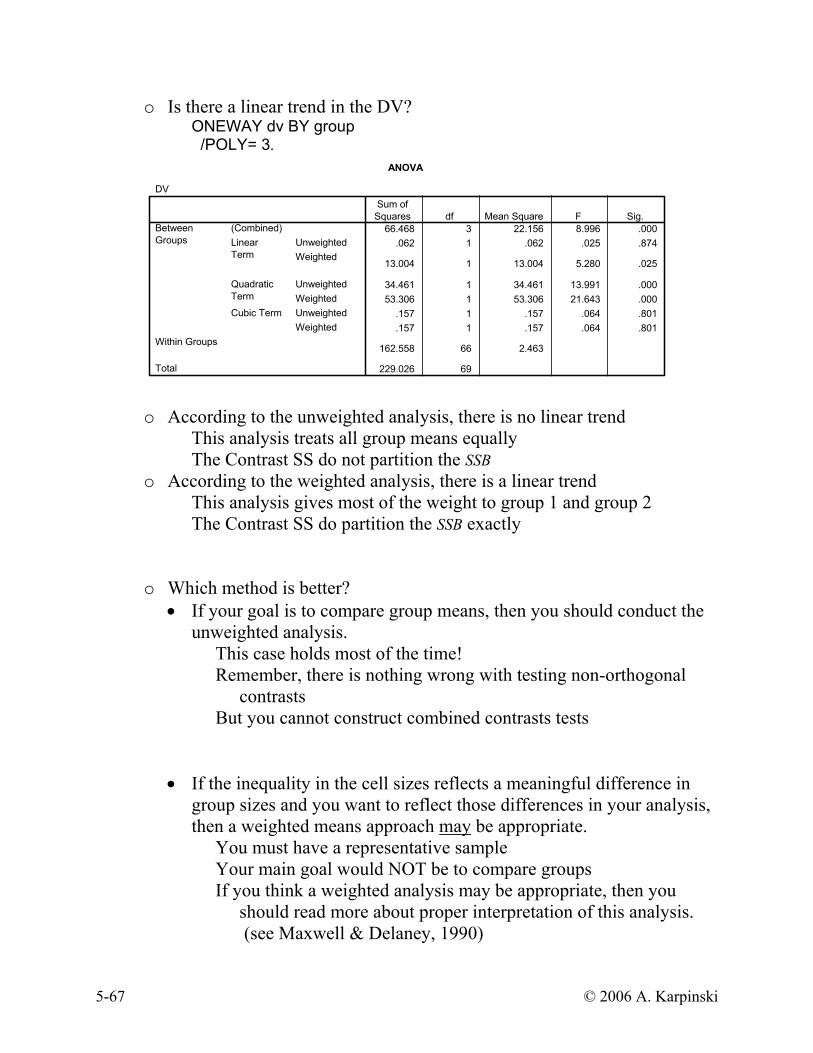
o Is there a linear trend in the DV? ONEWAY dv BY group /POLY= 3.
ANOVA
DV
66.468 3 22.156 8.996 .000.062 1 .062 .025 .874
13.004 1 13.004 5.280 .025
34.461 1 34.461 13.991 .00053.306 1 53.306 21.643 .000
.157 1 .157 .064 .801
.157 1 .157 .064 .801
162.558 66 2.463
229.026 69
(Combined)UnweightedWeighted
LinearTerm
UnweightedWeighted
QuadraticTerm
UnweightedWeighted
Cubic Term
BetweenGroups
Within Groups
Total
Sum ofSquares df Mean Square F Sig.
o According to the unweighted analysis, there is no linear trend This analysis treats all group means equally The Contrast SS do not partition the SSB
o According to the weighted analysis, there is a linear trend This analysis gives most of the weight to group 1 and group 2 The Contrast SS do partition the SSB exactly
o Which method is better?
• If your goal is to compare group means, then you should conduct the unweighted analysis.
This case holds most of the time! Remember, there is nothing wrong with testing non-orthogonal
contrasts But you cannot construct combined contrasts tests
• If the inequality in the cell sizes reflects a meaningful difference in
group sizes and you want to reflect those differences in your analysis, then a weighted means approach may be appropriate.
You must have a representative sample Your main goal would NOT be to compare groups If you think a weighted analysis may be appropriate, then you
should read more about proper interpretation of this analysis. (see Maxwell & Delaney, 1990)
5-68 © 2006 A. Karpinski
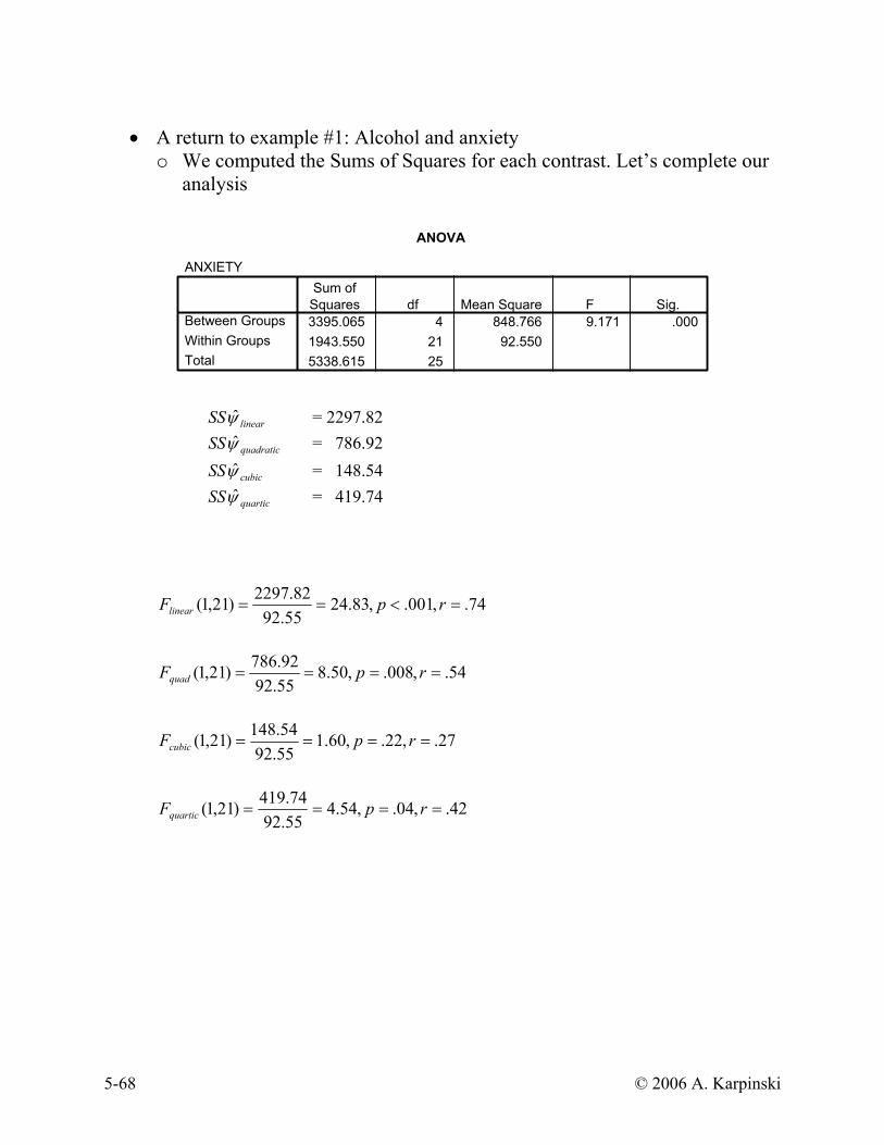
• A return to example #1: Alcohol and anxiety
o We computed the Sums of Squares for each contrast. Let’s complete our analysis
ANOVA
ANXIETY
3395.065 4 848.766 9.171 .0001943.550 21 92.5505338.615 25
Between GroupsWithin GroupsTotal
Sum ofSquares df Mean Square F Sig.
SS linearψ̂ = 2297.82 SS quadraticψ̂ = 786.92 SS cubicψ̂ = 148.54 SS quarticψ̂ = 419.74
74.,001.,83.2455.92
82.2297)21,1( =<== rpFlinear
54.,008.,50.8
55.9292.786)21,1( ==== rpFquad
27.,22.,60.1
55.9254.148)21,1( ==== rpFcubic
42.,04.,54.4
55.9274.419)21,1( ==== rpFquartic
5-69 © 2006 A. Karpinski
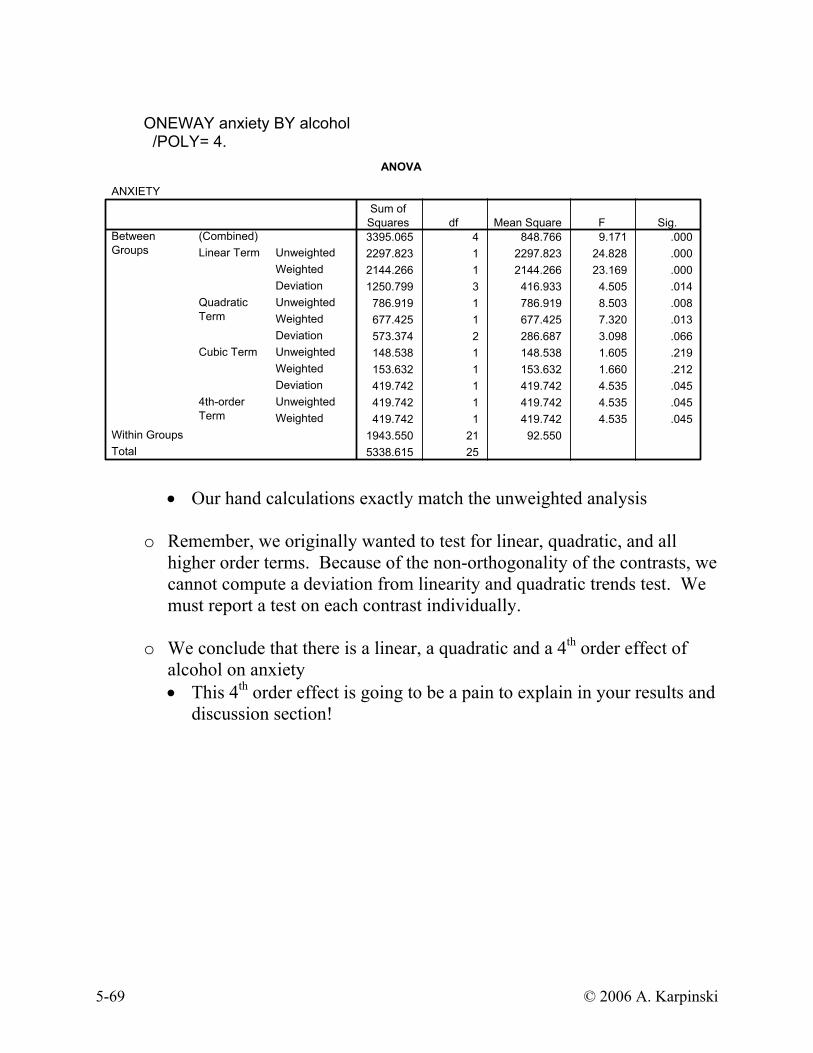
ONEWAY anxiety BY alcohol /POLY= 4.
ANOVA
ANXIETY
3395.065 4 848.766 9.171 .0002297.823 1 2297.823 24.828 .0002144.266 1 2144.266 23.169 .0001250.799 3 416.933 4.505 .014
786.919 1 786.919 8.503 .008677.425 1 677.425 7.320 .013573.374 2 286.687 3.098 .066148.538 1 148.538 1.605 .219153.632 1 153.632 1.660 .212419.742 1 419.742 4.535 .045419.742 1 419.742 4.535 .045419.742 1 419.742 4.535 .045
1943.550 21 92.5505338.615 25
(Combined)UnweightedWeightedDeviation
Linear Term
UnweightedWeightedDeviation
QuadraticTerm
UnweightedWeightedDeviation
Cubic Term
UnweightedWeighted
4th-orderTerm
BetweenGroups
Within GroupsTotal
Sum ofSquares df Mean Square F Sig.
• Our hand calculations exactly match the unweighted analysis
o Remember, we originally wanted to test for linear, quadratic, and all higher order terms. Because of the non-orthogonality of the contrasts, we cannot compute a deviation from linearity and quadratic trends test. We must report a test on each contrast individually.
o We conclude that there is a linear, a quadratic and a 4th order effect of
alcohol on anxiety • This 4th order effect is going to be a pain to explain in your results and
discussion section!

5-70 © 2006 A. Karpinski
12. A final example
• In an investigation of altruism in children, investigators examined children in 1st, 3rd, 4th, 5th, and 7th grades. The children were given a generosity scale. Below are the data collected:
Grade
1st 3rd 4th 5th 7th 0 1 3 2 2 1 3 0 3 2 1 3 0 1 0 2 2 3 0 1 0 2 2 3 1 1 3 1 2 2 2 2 2 0 0 2 1 1 1 3 0 1 1 0 1 0 2 2 3 1
1010101010N =
GRADE
7.005.004.003.001.00
ALT
RU
ISM
3.5
3.0
2.5
2.0
1.5
1.0
.5
0.0
-.5
1.00 3.00 5.00 7.00
grade
0.00
1.00
2.00
3.00al
trui
sm
A
A
A
A
A
A
A
AA
A
A
A
AA
A
A
A
A
AA
A
A
A
A
AA
A
A
A
A
A
A
A
A
A
A
A
AA
A
A
A
A
A
A
A
A
A
A
A
A
A
A
A A
o We want to investigate if there is a linear increase in altruism • The cell sizes are equal • But the spacing is not

5-71 © 2006 A. Karpinski
o We cannot use the tabled values for trend contrasts. We must let SPSS
compute them for us
UNIANOVA altruism BY grade /CONTRAST (grade)=Polynomial (1,3,4,5,7) /PRINT = test(lmatrix).
Tests of Between-Subjects Effects
Dependent Variable: ALTRUISM
5.120a 4 1.280 1.220 .316103.680 1 103.680 98.847 .000
5.120 4 1.280 1.220 .31647.200 45 1.049
156.000 5052.320 49
SourceCorrected ModelInterceptGRADEErrorTotalCorrected Total
Type III Sumof Squares df Mean Square F Sig.
R Squared = .098 (Adjusted R Squared = .018)a.
Contrast Coefficients (L' Matrix)
.000 .000 .000 .000-.671 .546 -.224 4.880E-02-.224 -.327 .671 -.439.000 -.436 .000 .781.224 -.327 -.671 -.439.671 .546 .224 4.880E-02
ParameterIntercept[GRADE=1.00][GRADE=3.00][GRADE=4.00][GRADE=5.00][GRADE=7.00]
Linear Quadratic Cubic Order 4
GRADE Polynomial Contrasta
The default display of this matrix is the transpose of thecorresponding L matrix.
Metric = 1.000, 3.000, 4.000, 5.000, 7.000a.

5-72 © 2006 A. Karpinski
Contrast Results (K Matrix)
.4920
.492
.324
.136-.1601.144
.1530
.153
.324
.639-.500.805
-.1340
-.134
.324
.681-.786.518
-.4780
-.478
.324
.147-1.130
.174
Contrast EstimateHypothesized ValueDifference (Estimate - Hypothesized)
Std. ErrorSig.
Lower BoundUpper Bound
95% Confidence Intervalfor Difference
Contrast EstimateHypothesized ValueDifference (Estimate - Hypothesized)
Std. ErrorSig.
Lower BoundUpper Bound
95% Confidence Intervalfor Difference
Contrast EstimateHypothesized ValueDifference (Estimate - Hypothesized)
Std. ErrorSig.
Lower BoundUpper Bound
95% Confidence Intervalfor Difference
Contrast EstimateHypothesized ValueDifference (Estimate - Hypothesized)
Std. ErrorSig.
Lower BoundUpper Bound
95% Confidence Intervalfor Difference
GRADE PolynomialContrasta
Linear
Quadratic
Cubic
Order 4
ALTRUISM
Dependent Variable
Metric = 1.000, 3.000, 4.000, 5.000, 7.000a.
o We find no evidence for any trends in the data,
all F’s(1, 45) < 2.31, p’s > .13
• The purpose of the study was to examine linear trends, so can I test the linear trend and the deviation from a linear trend?
o Can I use the ONEWAY command to do so?

5-73 © 2006 A. Karpinski
ONEWAY altruism BY grade /POLYNOMIAL= 1.
ANOVA
ALTRUISM
5.120 4 1.280 1.220 .3162.420 1 2.420 2.307 .136
2.700 3 .900 .858 .470
47.200 45 1.04952.320 49
(Combined)ContrastDeviation
Linear TermBetweenGroups
Within GroupsTotal
Sum ofSquares df Mean Square F Sig.
• Yes, but only if we have grade coded as (1, 3, 4, 5, 7). Remember, ONEWAY uses the spacing provided in your coding of the data
• We can report no evidence of a linear trend, 03.,14.,31.2)45,1( 2 === ωpF , and no evidence for any higher order
trends, 01.,47.,86.0)45,3( 2 <== ωpF