5.1

Chapter 5: Circuit Theorems This chapter provides a new powerful technique of solving complicated circuits that are more conceptual in nature than node/mesh analysis. Conceptually, the method is fairly straightforward to write down, however, they are complicated to apply in practice. One will find that the amount of work increases dramatically using these circuit theorems to solve a circuit. There are four theorems we will look at in this chapter: Source Transformations, Superposition Principle and Thévenin & Norton Equivalents, and Maximum Power Theorem. There are two useful ideas to take away from this chapter.

1. Thévenin-Norton source transformations. In certain situations, there is a way to convert a voltage source into a current source and vice-versa. Source transformations are going to change how you solve circuits and in some cases, a series of source transformations will have a dramatic affect in making the circuit calculation quite straight forward. Source transformations will become an additional technique in your arsenal in solving circuits regardless of the techniques one uses (SCT, Node, Mesh…).

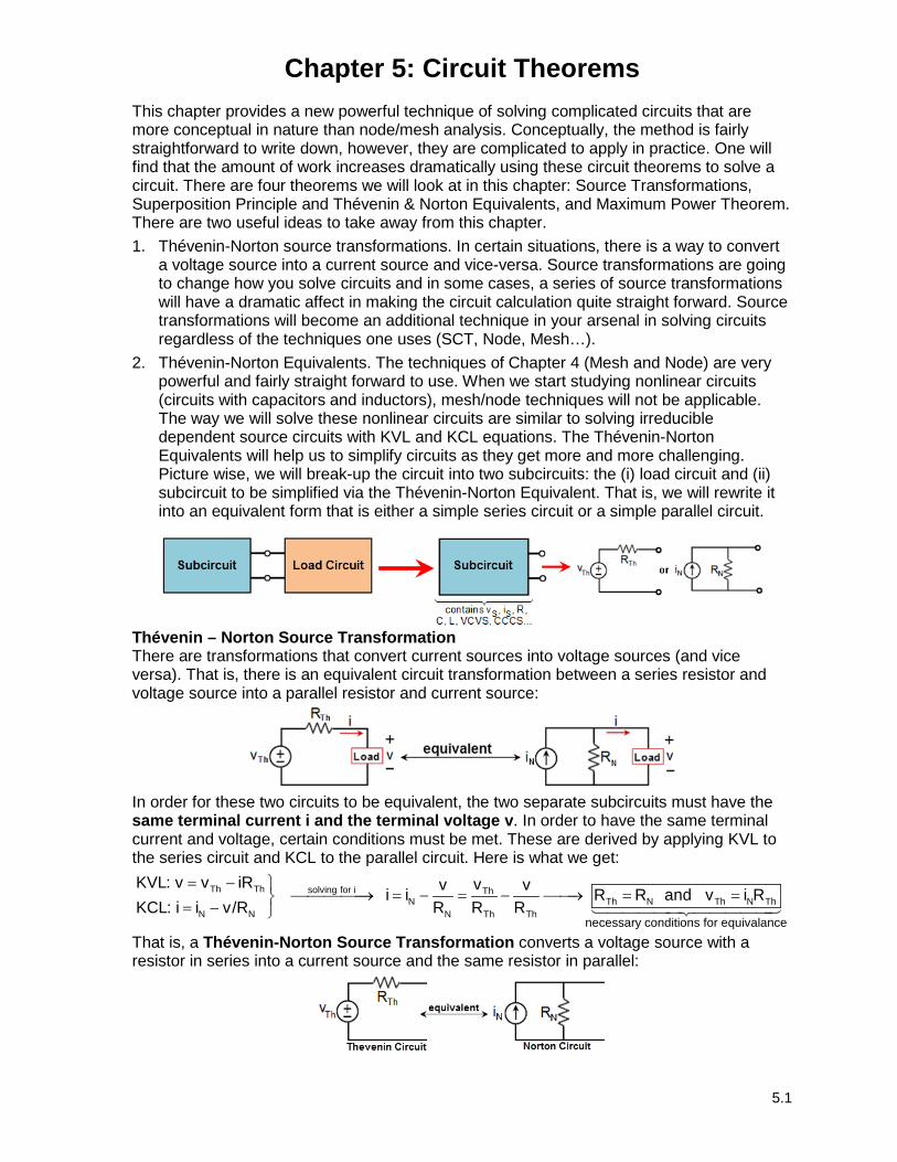
2. Thévenin-Norton Equivalents. The techniques of Chapter 4 (Mesh and Node) are very powerful and fairly straight forward to use. When we start studying nonlinear circuits (circuits with capacitors and inductors), mesh/node techniques will not be applicable. The way we will solve these nonlinear circuits are similar to solving irreducible dependent source circuits with KVL and KCL equations. The Thévenin-Norton Equivalents will help us to simplify circuits as they get more and more challenging. Picture wise, we will break-up the circuit into two subcircuits: the (i) load circuit and (ii) subcircuit to be simplified via the Thévenin-Norton Equivalent. That is, we will rewrite it into an equivalent form that is either a simple series circuit or a simple parallel circuit.

Thévenin – Norton Source Transformation There are transformations that convert current sources into voltage sources (and vice versa). That is, there is an equivalent circuit transformation between a series resistor and voltage source into a parallel resistor and current source:

In order for these two circuits to be equivalent, the two separate subcircuits must have the same terminal current i and the terminal voltage v. In order to have the same terminal current and voltage, certain conditions must be met. These are derived by applying KVL to the series circuit and KCL to the parallel circuit. Here is what we get:

Th Th solving for i ThN Th N Th N Th

N N N Th Thnecessary conditions for equivalance

KVL: v v iR vv v i i R R and v i RKCL: i i v/R R R R

= − → = − = − → = == −

That is, a Thévenin-Norton Source Transformation converts a voltage source with a resistor in series into a current source and the same resistor in parallel:

5.2

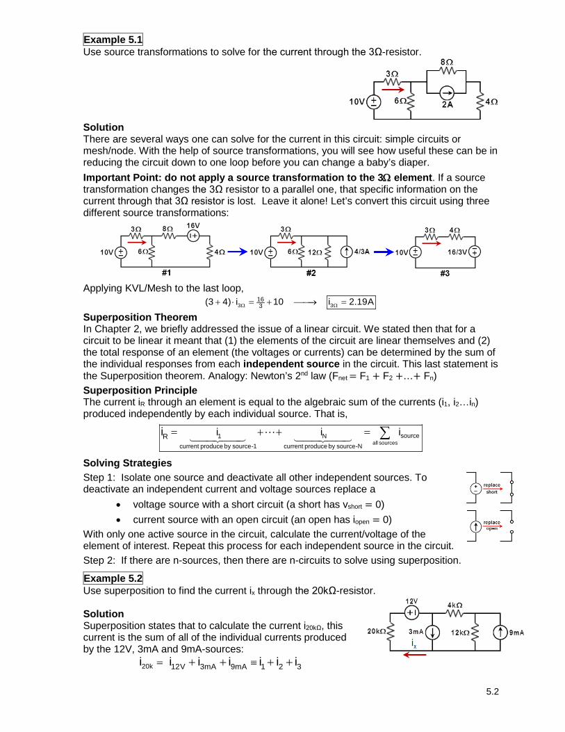
Example 5.1 Use source transformations to solve for the current through the 3Ω-resistor.

Solution There are several ways one can solve for the current in this circuit: simple circuits or mesh/node. With the help of source transformations, you will see how useful these can be in reducing the circuit down to one loop before you can change a baby’s diaper. Important Point: do not apply a source transformation to the 3Ω element. If a source transformation changes the 3Ω resistor to a parallel one, that specific information on the current through that 3Ω resistor is lost. Leave it alone! Let’s convert this circuit using three different source transformations:

Applying KVL/Mesh to the last loop,

3 3163(3 4) i 10 i 2.19AΩ Ω+ ⋅ = + → =

Superposition Theorem In Chapter 2, we briefly addressed the issue of a linear circuit. We stated then that for a circuit to be linear it meant that (1) the elements of the circuit are linear themselves and (2) the total response of an element (the voltages or currents) can be determined by the sum of the individual responses from each independent source in the circuit. This last statement is the Superposition theorem. Analogy: Newton’s 2nd law (Fnet = F1 + F2 +…+ Fn) Superposition Principle The current iR through an element is equal to the algebraic sum of the currents (i1, i2…in) produced independently by each individual source. That is,

all sources

source1 Ncurrent produce by source-1 current produce by source-N

R i i ii = + + = ∑

Solving Strategies Step 1: Isolate one source and deactivate all other independent sources. To deactivate an independent current and voltage sources replace a

• voltage source with a short circuit (a short has vshort = 0) • current source with an open circuit (an open has iopen = 0)

With only one active source in the circuit, calculate the current/voltage of the element of interest. Repeat this process for each independent source in the circuit. Step 2: If there are n-sources, then there are n-circuits to solve using superposition.

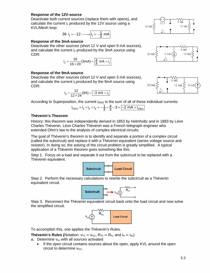
Example 5.2 Use superposition to find the current ix through the 20kΩ-resistor.

Solution Superposition states that to calculate the current i20kΩ, this current is the sum of all of the individual currents produced by the 12V, 3mA and 9mA-sources:

20k 12V 3mA 9mA 1 2 3i i i i i i i= ≡+ + + +

5.3

Response of the 12V-source Deactivate both current sources (replace them with opens), and calculate the current i1 produced by the 12V source using a KVL/Mesh loop:

1 11336 i 12 i mA⋅ →= − = −

Response of the 3mA-source Deactivate the other sources (short 12 V and open 9 mA sources), and calculate the current i2 produced by the 3mA source using CDR:

2243

16i (3mA) mA i16 + 20

= = =

Response of the 9mA-source Deactivate the other sources (short 12 V and open 3 mA sources), and calculate the current i3 produced by the 9mA source using CDR:

3312i (9A) 3 mA i

12 + 24= = − =

According to Superposition, the current i20kΩ is the sum of all of these individual currents:

20k 20k1 2 31 43 3i i i i 3 2 mA iΩ Ω= + + = − + − = − =

Thévenin’s Theorem

History: this theorem was independently derived in 1853 by Helmholtz and in 1883 by Léon Charles Thévenin. Léon Charles Thévenin was a French telegraph engineer who extended Ohm's law to the analysis of complex electrical circuits.

The goal of Thévenin’s theorem is to identify and separate a portion of a complex circuit (called the subcircuit) and replace it with a Thévenin equivalent (series voltage source and resistor). In doing so, the solving of the circuit problem is greatly simplified. A typical application of a Thévenin theorem goes something like this:

Step 1. Focus on a load and separate it out from the subcircuit to be replaced with a Thévenin equivalent.

Step 2. Perform the necessary calculations to rewrite the subcircuit as a Thévenin equivalent circuit.

Step 3. Reconnect the Thévenin equivalent circuit back onto the load circuit and now solve the simplified circuit.

To accomplish this, one applies the Thévenin’s Rules.

Thévenin’s Rules (Notation: vTh = vOC, RTh = RN, and iN = iSc) a. Determine voc with all sources activated

• If the open circuit contains sources about the open, apply KVL around the open circuit to determine vOC.

5.4

• Use any method to solve for vOC b. Determine RTh.

Method-1: Independent Sources Only (Conceptual Approach) Deactivate all sources and determine RTh relative to the terminal points a-b.

Method-2: Independent & Dependent Sources (Calculational Approach) i. Place a short at the terminal points a-b and calculate isc using any method. ii. Determine RTh by using RTh = vOC/iSC.

c. Redraw the equivalent Thévenin circuit. If the Thévenin resistance is negative, subtract it from the load resistance.

Dependent sources only – the book does not give any problems related to only dependent sources. I will not cover them; however, if you are transferring to San Jose State and plan on majoring in EE, at the end of the semester I can teach you these in about 10-15 minutes.

Independent Sources Only Because this example circuit only has an independent source, I will not only demonstrate how a Thévenin equivalent is determine between points a-b, but also show that Method-1 and Method-2 are equivalent.

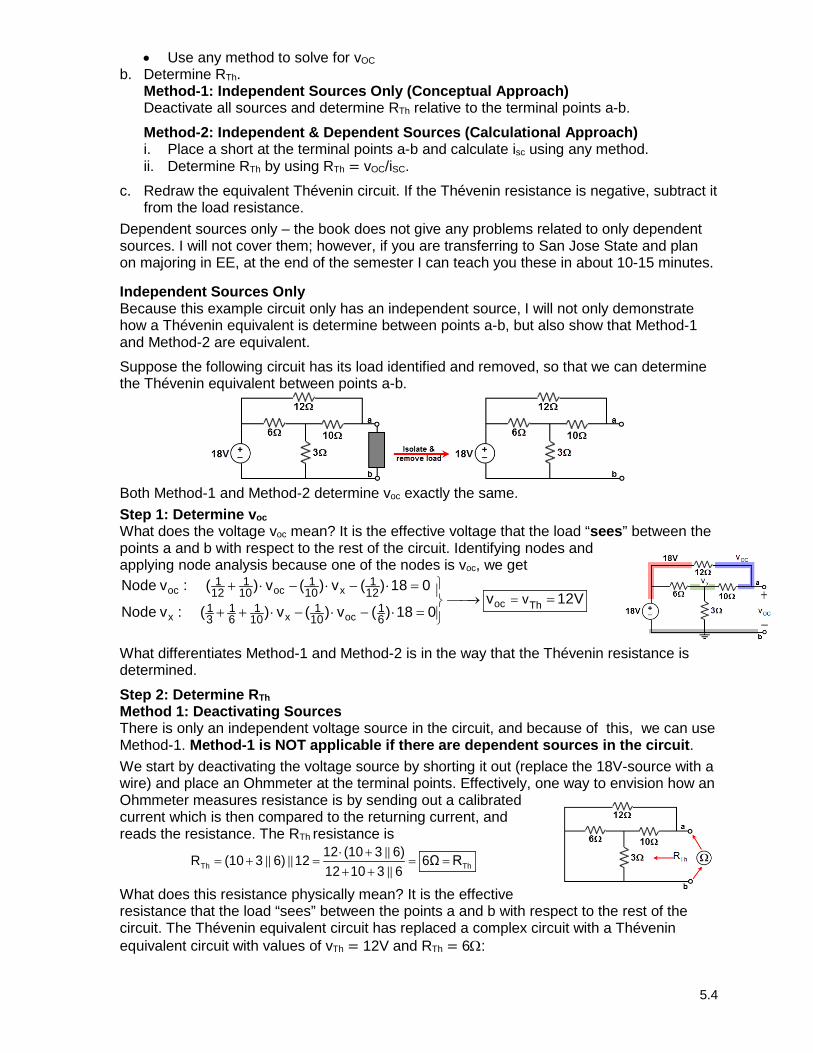
Suppose the following circuit has its load identified and removed, so that we can determine the Thévenin equivalent between points a-b.

Both Method-1 and Method-2 determine voc exactly the same.

Step 1: Determine voc What does the voltage voc mean? It is the effective voltage that the load “sees” between the points a and b with respect to the rest of the circuit. Identifying nodes and applying node analysis because one of the nodes is voc, we get

oc oc xoc Th

x x oc

1 1 1 112 10 10 12

1 1 1 1 13 6 10 10 6

vNode v : ( ) v ( ) v ( ) 18 0

v 12VNode v : ( ) v ( ) v ( ) 18 0

→ =

+ ⋅ − ⋅ − ⋅ ==

+ + ⋅ − ⋅ − ⋅ =

What differentiates Method-1 and Method-2 is in the way that the Thévenin resistance is determined.

Step 2: Determine RTh Method 1: Deactivating Sources There is only an independent voltage source in the circuit, and because of this, we can use Method-1. Method-1 is NOT applicable if there are dependent sources in the circuit.

We start by deactivating the voltage source by shorting it out (replace the 18V-source with a wire) and place an Ohmmeter at the terminal points. Effectively, one way to envision how an Ohmmeter measures resistance is by sending out a calibrated current which is then compared to the returning current, and reads the resistance. The RTh resistance is

Th Th12 (10 3 6)R (10 3 6) 12 6Ω R12 10 3 6

⋅ += + = = =

+ +

What does this resistance physically mean? It is the effective resistance that the load “sees” between the points a and b with respect to the rest of the circuit. The Thévenin equivalent circuit has replaced a complex circuit with a Thévenin equivalent circuit with values of vTh = 12V and RTh = 6Ω:

5.5

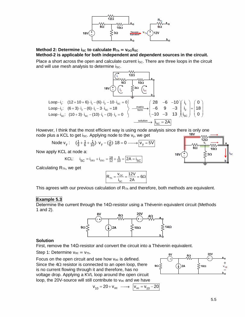
Method 2: Determine iSC to calculate RTh = vOC/iSC Method-2 is applicable for both independent and dependent sources in the circuit.

Place a short across the open and calculate current iSC. There are three loops in the circuit and will use mesh analysis to determine iSC.

1 1 2 SC

2 2 1 SC

SC SC 1 2

1matrix

2form

SC

Loop - i : (12 10 6) i (6) i 10 i 0Loop - i : (6 3) i (6) i 3 i 18Loop - i : (10 3) i (10) i (3) i 0

28 6 10 i 0 6 9 3 i 18

10 3 13 i 0

+ + ⋅ − ⋅ − ⋅ = + ⋅ − ⋅ − ⋅ = → =

+ ⋅ − ⋅ − ⋅ =

− −− −

− −solution

SC

i 2A

→ =

However, I think that the most efficient way is using node analysis since there is only one node plus a KCL to get iSC. Applying node to the vy, we get

y y y1 1 1 13 6 10 6 5Node v : ( ) v ( ) 18 0 v V→ =+ + ⋅ − ⋅ =

Now apply KCL at node a:

18 1018 5

SC SC12 10KCL i i i 2A i: Ω Ω+ = + = ==

Calculating RTh, we get OC

ThSC

v 12VR 6i 2A

= = = Ω

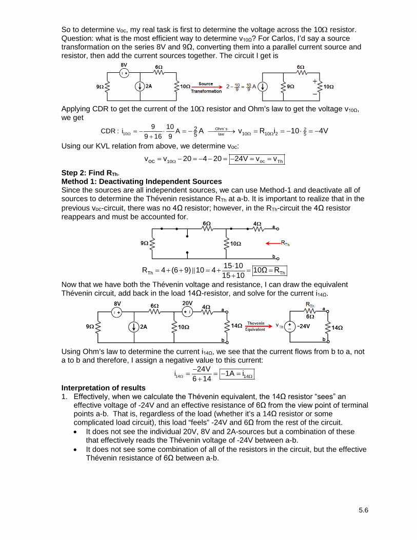
This agrees with our previous calculation of RTh and therefore, both methods are equivalent. Example 5.3 Determine the current through the 14Ω-resistor using a Thévenin equivalent circuit (Methods 1 and 2).

Solution First, remove the 14Ω-resistor and convert the circuit into a Thévenin equivalent. Step 1: Determine voc = vTh. Focus on the open circuit and see how voc is defined. Since the 4Ω resistor is connected to an open loop, there is no current flowing through it and therefore, has no voltage drop. Applying a KVL loop around the open circuit loop, the 20V-source will still contribute to voc and we have

ococ10 10v 20 v v v 20→= + = −

5.6

So to determine voc, my real task is first to determine the voltage across the 10Ω resistor. Question: what is the most efficient way to determine v10Ω? For Carlos, I’d say a source transformation on the series 8V and 9Ω, converting them into a parallel current source and resistor, then add the current sources together. The circuit I get is

Applying CDR to get the current of the 10Ω resistor and Ohm’s law to get the voltage v10Ω, we get

Ohm's10 law

210 10 2 5

25

9 10CDR : i A 9 16 9

A v R i 10 4VΩ Ω Ω= − ⋅ →+

= − = = − ⋅ = −

Using our KVL relation from above, we determine voc:

oc10 Thocv v 20 4 20 24V v vΩ= − = − − = − = =

Step 2: Find RTh. Method 1: Deactivating Independent Sources Since the sources are all independent sources, we can use Method-1 and deactivate all of sources to determine the Thévenin resistance RTh at a-b. It is important to realize that in the previous voc-circuit, there was no 4Ω resistor; however, in the RTh-circuit the 4Ω resistor reappears and must be accounted for.

Th Th15 10R 4 (6 9) 10 4 10Ω R15 10

⋅= + + = + = =+

Now that we have both the Thévenin voltage and resistance, I can draw the equivalent Thévenin circuit, add back in the load 14Ω-resistor, and solve for the current i14Ω.

Using Ohm’s law to determine the current i14Ω, we see that the current flows from b to a, not a to b and therefore, I assign a negative value to this current:

14 14i 24V 1A i6 14Ω Ω−= = − =

+

Interpretation of results 1. Effectively, when we calculate the Thévenin equivalent, the 14Ω resistor “sees” an

effective voltage of -24V and an effective resistance of 6Ω from the view point of terminal points a-b. That is, regardless of the load (whether it’s a 14Ω resistor or some complicated load circuit), this load “feels” -24V and 6Ω from the rest of the circuit. • It does not see the individual 20V, 8V and 2A-sources but a combination of these

that effectively reads the Thévenin voltage of -24V between a-b. • It does not see some combination of all of the resistors in the circuit, but the effective

Thévenin resistance of 6Ω between a-b.

5.7

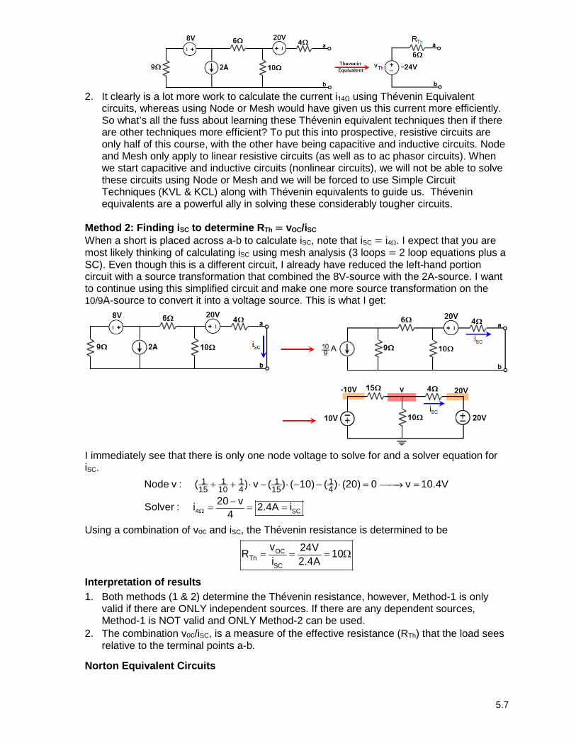
2. It clearly is a lot more work to calculate the current i14Ω using Thévenin Equivalent

circuits, whereas using Node or Mesh would have given us this current more efficiently. So what’s all the fuss about learning these Thévenin equivalent techniques then if there are other techniques more efficient? To put this into prospective, resistive circuits are only half of this course, with the other have being capacitive and inductive circuits. Node and Mesh only apply to linear resistive circuits (as well as to ac phasor circuits). When we start capacitive and inductive circuits (nonlinear circuits), we will not be able to solve these circuits using Node or Mesh and we will be forced to use Simple Circuit Techniques (KVL & KCL) along with Thévenin equivalents to guide us. Thévenin equivalents are a powerful ally in solving these considerably tougher circuits.

Method 2: Finding iSC to determine RTh = vOC/iSC When a short is placed across a-b to calculate iSC, note that iSC = i4Ω. I expect that you are most likely thinking of calculating iSC using mesh analysis (3 loops = 2 loop equations plus a SC). Even though this is a different circuit, I already have reduced the left-hand portion circuit with a source transformation that combined the 8V-source with the 2A-source. I want to continue using this simplified circuit and make one more source transformation on the 10/9A-source to convert it into a voltage source. This is what I get:

I immediately see that there is only one node voltage to solve for and a solver equation for iSC.

4 SC

1 1 1 1 14 415 10 15Node v : ( ) v ( ) ( 10) ( ) (20) 0 v 10.4V

20 vSolver : i 2.4A i4Ω

→+ + ⋅ − ⋅ − − ⋅ = =

−= = =

Using a combination of voc and iSC, the Thévenin resistance is determined to be

OCTh

SC

v 24VR 10i 2.4A

= = = Ω

Interpretation of results 1. Both methods (1 & 2) determine the Thévenin resistance, however, Method-1 is only

valid if there are ONLY independent sources. If there are any dependent sources, Method-1 is NOT valid and ONLY Method-2 can be used.

2. The combination voc/iSC, is a measure of the effective resistance (RTh) that the load sees relative to the terminal points a-b.

Norton Equivalent Circuits

5.8

Independent & Dependent Sources

There are two important changes when dealing with independent and dependent sources in circuit where Thévenin’s theorem is going to be applied: 1. Without dependent sources, zeroing all the independent sources leaves a resistive

circuit so that the Thévenin resistance can be calculated directly. However, dependent sources typically alter the Thévenin resistance so those can't be zeroed. That is, Method-1 is NOT VALID whenever dependent sources are in the circuit and the only way to determine RTh is by using Medthod-2; determine the ratio vOC/iSC = RTh.

2. Thévenin circuit with dependent sources can have positive and negative Thévenin resistance. It is not like there is an actual negative resistor that one can actual purchase at the store or something like that, but has implications that circuits have a “impedance matching” and can be “resonated.”

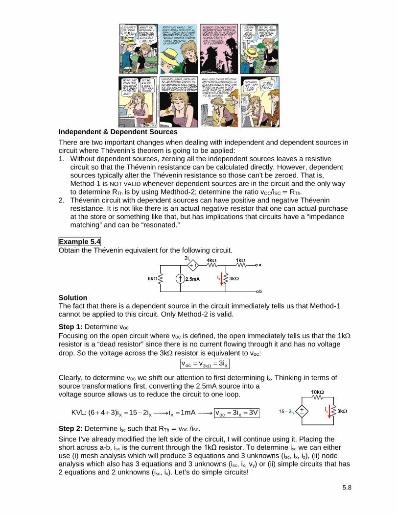
Example 5.4 Obtain the Thévenin equivalent for the following circuit.

Solution The fact that there is a dependent source in the circuit immediately tells us that Method-1 cannot be applied to this circuit. Only Method-2 is valid.

Step 1: Determine voc Focusing on the open circuit where voc is defined, the open immediately tells us that the 1kΩ resistor is a “dead resistor” since there is no current flowing through it and has no voltage drop. So the voltage across the 3kΩ resistor is equivalent to voc:

3k Xocv v 3iΩ= =

Clearly, to determine voc we shift our attention to first determining ix. Thinking in terms of source transformations first, converting the 2.5mA source into a voltage source allows us to reduce the circuit to one loop.

: X X X XocKVL (6 4 3)i 15 2i i 1mA v 3i 3V→ →+ + = − = = =

Step 2: Determine isc such that RTh = voc /isc.

Since I’ve already modified the left side of the circuit, I will continue using it. Placing the short across a-b, isc is the current through the 1kΩ resistor. To determine isc we can either use (i) mesh analysis which will produce 3 equations and 3 unknowns (isc, ix, iz), (ii) node analysis which also has 3 equations and 3 unknowns (isc, ix, vy) or (ii) simple circuits that has 2 equations and 2 unknowns (isc, ix). Let’s do simple circuits!

5.9

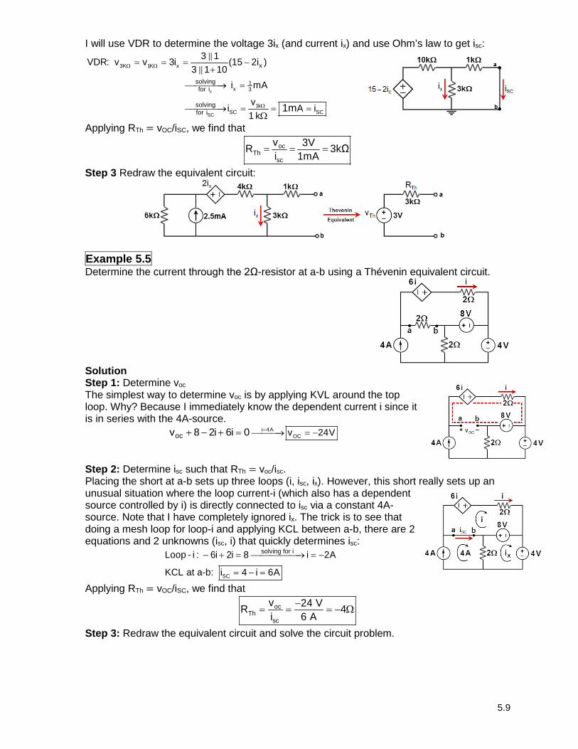
I will use VDR to determine the voltage 3ix (and current ix) and use Ohm’s law to get isc:

x

SC

3K 1K x

1x 3

1kSC SC

x

solvingfor i

solvingfor i

3 1VDR: v v 3i (15 2i )3 1 10

i mA

v i A i1 k

1m

Ω Ω

Ω

= = = −+

→ =

→ = = =Ω

Applying RTh = vOC/iSC, we find that oc

Thsc

v 3VR 3kΩi 1mA

= = =

Step 3 Redraw the equivalent circuit:

Example 5.5 Determine the current through the 2Ω-resistor at a-b using a Thévenin equivalent circuit.

Solution Step 1: Determine voc The simplest way to determine voc is by applying KVL around the top loop. Why? Because I immediately know the dependent current i since it is in series with the 4A-source.

i 4AOCoc v 24Vv 8 2i 6i 0 =→ = −+ − + =

Step 2: Determine isc such that RTh = voc/isc. Placing the short at a-b sets up three loops (i, isc, ix). However, this short really sets up an unusual situation where the loop current-i (which also has a dependent source controlled by i) is directly connected to isc via a constant 4A-source. Note that I have completely ignored ix. The trick is to see that doing a mesh loop for loop-i and applying KCL between a-b, there are 2 equations and 2 unknowns (isc, i) that quickly determines isc:

SC

solving for iLoop - i : 6i 2i 8 i 2A

KCL at a-b: i 4 i 6A

− + = → = −

= − =

Applying RTh = vOC/iSC, we find that oc

Thsc

v 24 VR 4i 6 A

−= = = − Ω

Step 3: Redraw the equivalent circuit and solve the circuit problem.

5.10

Using Ohm’s law, the current through the 2-resistor is OC

2 2Th

v 24i 12 A iR 2 4 2Ω Ω

−= = = =

+ Ω − +

Because this current is positive, the current runs positive from terminal a to terminal b.

Interpretation of Negative Thévenin Resistance Suppose now that the load resistor was replaced with a variable resistor (i.e., decade resistor box) such that we adjusted the resistance. How does the circuit behave?

One would think that if one sets Rab = 0Ω, then maximum current would flow through the load resistance Rab. Let’s look at this:

OCload

Th load

v 24i 6 AR R 4 0

−= = = −

+ − +

If I now adjusted the decade resistor box to Rload = 2Ω, the current now reads 12A, double the value of the short circuit current:

load24i 12 A

4 2−

= = −− +

And as you can see, something very special happens as Rload → 4Ω, the current goes to infinity:

load loadloadR 4 R 4

load

24lim i lim4 R→ Ω → Ω

−= →∞

− +

Physical interpretation The key phase is “impedance matching.” Negative resistance cannot physically occur in the case where the circuit is linear and contains only passive components (resistors, capacitors and inductors). But for active circuits, where dependent sources (amplifiers) are applied, a virtual negative resistance can be realized. The physical meaning of negative resistance is that power is absorbed by the circuit with zero phase shift rather than dissipated. Maximum Power Delivered to a Circuit The Maximum Power Transfer Theorem is not so much a means of analysis as it is an aid to system design. Simply stated, the maximum amount of power will be dissipated by a load resistance when that load resistance is equal to the Thévenin resistance of the circuit supplying the power. If the load resistance is lower or higher than the Thévenin resistance, its dissipated power will be less than maximum.

This is essentially what is aimed for in radio transmitter design where the antenna or transmission line “impedance” is matched to final power amplifier “impedance” for maximum radio frequency power output (impedance matching). Impedance, the overall opposition to AC and DC current, is very similar to resistance, and must be equal between source and load for the greatest amount of power to be transferred to the load. A load impedance that is too high will result in low power output. A load impedance that is too low will not only result in low power output, but possibly overheating of the amplifier due to the power dissipated in its internal Thévenin impedance.

Mathematically, one can determine the maximum power delivered to the load by calculating the critical point where dPload/dRload = 0:

5.11

( )

22load load load load

load Th load Th 2Th load load load load Th load

R v dP Rdv v P v 0R R R dR dR R R

= → = → = = + +

After doing some algebra, we arrive

( ) ( )load Th load load

Th load2 4load Th load Th load

R R R 2Rd 0 R RdR R R R R

+ − = = → = + +

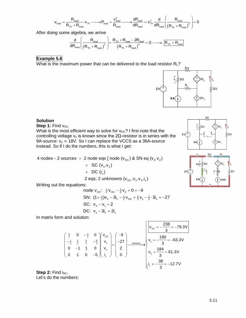
Example 5.6 What is the maximum power that can be delivered to the load resistor RL?

Solution Step 1: Find vOC What is the most efficient way to solve for vOC? I first note that the controlling voltage vy is known since the 2Ω-resistor is in series with the 9A-source: vy = 18V. So I can replace the VCCS as a 36A-source instead. So if I do the numbers, this is what I get:

OC 1 2

1 2

x

4 nodes 2 sources 2 node eqs [ node (v ) & SN eq (v ,v ) SC (v ,v ) DC (i ) 2 eq

− =

+

+

OC 1 2 xs, 2 unknowns (v ,v ,v ,i )

Writing out the equations: 1 1

OC OC 22 21 1 1 1

2 x OC 1 x2 2 2 2

2 1

1 x x

node v : v v 0 9SN: (1 )v 3i v v 3i 27SC: v v 2DC: v 3i 2i

− + = −

+ − − + − ⋅ = −

− =

− =

In matrix form and solution:

OC

1 1OC2 2

3 91 1 11 solutions2 2 2 2

2

2x

x

238v 79.3V

3v 90 0 190

v 63.3Vv 27 3v 20 1 1 0 184

v 61.3Vi 00 1 0 5 3

38i 12.7V

3

= − = −

−−= − = −−− −

=−

= =−

= − = −

→

Step 2: Find iSC. Let’s do the numbers:

5.12

2 1 3 x

x y

4 loops 2 sources 2 loops eqs (1 regular (i ) & 1 SL (i ,i ,i )

2 SC DC (i , v )

− =

+

+

SC

1 2 3 x y SC

Solver (i )

6 eqs, 6 unknowns (i ,i ,i ,i ,v ,i )

+

Writing out the equations, ( )

x

3 1 3 x y

y 2 1

SC 2 3

x

x2loop iloop 1

2 1

x1 0

i i 9, i i 2vDC : v 2i 2iSolver : i i i

Loop 2 : 1 2 i 2i 3i SL: 2i 2i 2 i 3i 2

2 SC :

+

− = − =

= −

= −

+ − =

− + ⋅ = − −

The matrix and solutions are 11

22

33

xx

yy

SC SC

solutions

i 3.58Ai2 3 0 3 0 0 0i 2.26Ai2 2 0 5 0 0 2i 5.42Ai1 0 1 0 0 0 9i 0.129Ai0 0 1 1 2 0 0v 2.65Vv2 2 0 0 1 0 0

0 1 1 0 0 1 0i i 7.67A

= − − − − = −− − = − → =− − =− − − − = −

=

Step 3: Find RTH and solve the circuit problem Applying RTh = vOC/iSC, we find that

ocTh

sc

v 79.3VR 10.3 i 7.67A

−= = = Ω−

Th ThR 10.3 79.3V v= Ω = −

Th L max

2 2maximum power theorem L

maxR R 10.3L

v (79.3 / 2) 153 W PR 10.3

P= = Ω→ = = = =