chapter 5 - benjamin a....

Chapter 5

Applying

Consumer

theory

5 - 2 Copyright © 2012 Pearson Addison-Wesley. All rights reserved.

Topics

• Deriving Demand Curves.

• How Changes in Income Shift Demand Curves.

• Effects of a Price Change.

• Cost-of-Living Adjustments.

• Deriving Labor Supply Curves.


Figure 5.1 Deriving

an Individual’s

Demand Curve

26.70

Initial Values

Pb = price of beer = $12

PW = price of wine = $35

Y = Income = $419.

W = YPW

-PbPW

b

Budget Line, L

12.0

2.8

12.0

26.70

pb, $ p

er

unit

e1

E1

I1

Beer (b), Gallons per year

Win

e, (W

) , G

allo

ns p

eryear

(b) Demand Curve Initial optimal bundle of

beer and wine


L1 (pb = $12)

(a) Indifference Curves and Budget Constraints


Figure 5.1 Deriving

an Individual’s

Demand Curve

New Values



Y = Income = $419.

W = YPW

-PbPW

b

Budget Line, L

Price of beer goes down!

4.3

12.0

2.8

12.0

6.0

26.70

pb, $ p

er

unit

L2 (pb

= $6)

26.70 44.5

e2

e1

I1

I2


Win

e, (W

) , G

allo

ns p

eryear

(b) Demand Curve


L1 (pb = $12)

E1

44.5

E2



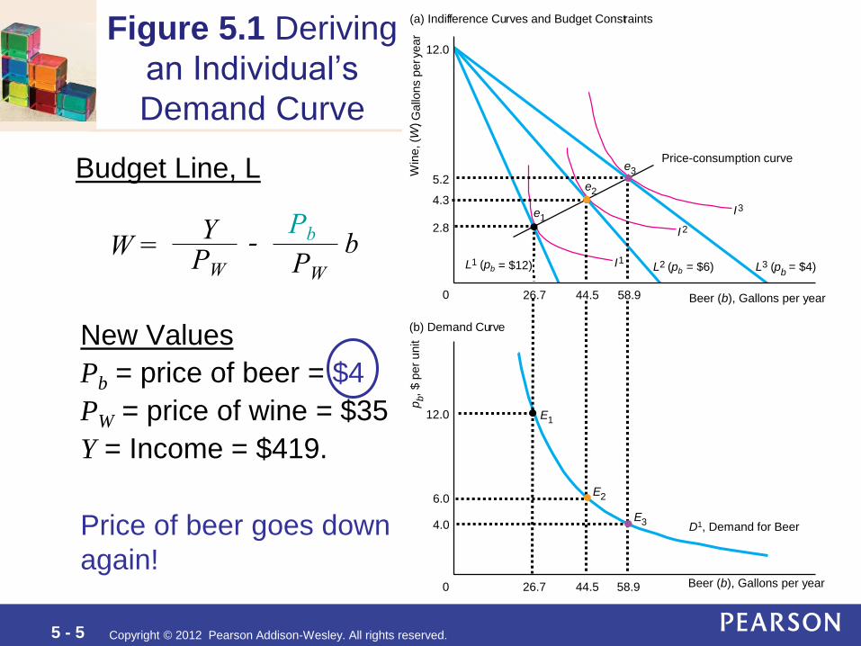
Figure 5.1 Deriving

an Individual’s

Demand Curve

New Values



Y = Income = $419.

W = YPW

-PbPW

b

Budget Line, L

Price of beer goes down

again!

4.3

5.2

12.0

2.8

12.0

6.0

4.0

26.70 44.5 58.9

pb, $ p

er

unit

L2 (pb = $6) L3 (pb

= $4)

26.70 44.5 58.9

e

e1

I1

I2

I3


D1, Demand for Beer

Price-consumption curve

Win

e, (W

) , G

allo

ns p

eryear


(b) Demand Curve


L1 (pb = $12)

E1

2

E2

e3

E3


Price-Consumption Curve

• A line through optimal bundles at each

price of one good (beer) when the price of

the other good (wine) and the budget are

held constant.

• The demand curve corresponds to the

price-consumption curve.


Effects of a Rise in Income

• Engel curve - the relationship between

the quantity demanded of a single good

and income, holding prices constant.

• Income-consumption curve shows how

consumption of both goods changes when

income changes, while prices are held

constant.


Y1

Figure 5.2 Effect of a

Budget Increase on an

Individual’s Demand Curve

Initial Values



Y = Income = $419.

W = YPW

-PW

b

Budget Line, L

Pb

Win

e, G

allo

ns p

er

year

0

2.8

26.7 Beer, Gallons per year

0

12

0



I1

Pri

ce o

f beer,

$ p

er

unit

Y, B

udget

E1

= $419

L1

e1

D1

E1*Income goes up!

$628


Initial Values



Y = Income = $419.

W = YPW

-PW

b

Budget Line, L

Pb

Income goes up!

$628

Win

e, G

allo

ns p

eryear

0

2.8

4.8

38.226.7 Beer, Gallons per year

0

12

0



I2

I1

Pri

ce o

f beer,

$ p

er

unit

Y, B

udget

e2

E1

Y1 = $419

Y2 = $628

L2

L1

e1

D1D2

E1*

E2

E2*





Y

Y

Y

Initial Values



Y = Income = $837.

W = YPW

-PW

b

Budget Line, L

Pb

Income goes up again!W

ine, G

allo

ns p

eryear

Income-consumption curve

Engel curve for beer

0

2.8

4.8

7.1

49.138.226.7 Beer, Gallons per year

0

12

0



I2I3

I1

Pri

ce o

f beer,

$ p

er

unit

Y, B

udget

e2

E1

1 = $419

2 = $628

3 = $837

L3

L2

L1

e1

D1D2D3

E1*

E2

E2*

E3

E3*

e3





Consumer Theory and Income Elasticities

• Formally,

where Y stands for income.

• Example

If a 1% increase in income results in a 3% decrease in

quantity demanded, the income elasticity of demand is

x = -3%/1% = -3.

Q

Y

Y

Q

Y

Y

Q

Q

Y

Q

%

%x


Consumer Theory and Income Elasticities

(cont.)

• Normal good - a commodity of which as

much or more is demanded as income

rises.

Positive income elasticity.

• Inferior good - a commodity of which less

is demanded as income rises.

Negative income elasticity.


Figure 5.3 Income-Consumption

Curves and Income Elasticities

• As income rises the budget constraint shifts to the right. The income

elasticities depend on….

• …where on the new budget constraint the new optimal consumption bundle will be

Ho

usin

g,

Sq

ua

refe

et

pery

ear

Food, Pounds peryear

Food normal,

housing normal

Food inferior,housing normal

Food normal,housing inferior

b

c

e

a

L1

L2

I

ICC2

ICC1

ICC3


Figure 5.4 A Good

That Is Both Inferior

and Normal

• When Gail was poor and her income increased..

…she bought more hamburger

• But as she became wealthier and her income rose…

….she bought less hamburger and more steak.

Y2

Y1

Y1

Y2

Y3

Y3

L1

Y,

Inco

me

L2

L3

e2

e3

e1

E2

E3

E1

I1

I 2

I 3

Hamburger peryear

Income-consumption curve

Hamburger peryear

yA

ll o

the

r go

od

s p

er

ea

r


(b) Engel Curve

Engel curve


Effects of a Price Change

• Substitution effect - the change in the quantity of a good that a consumer demands when the good’s price changes, holding other prices and the consumer’s utility constant.

• Income effect - the change in the quantity of a good a consumer demands because of a change in income, holding prices constant.


Figure 5.5 Substitution and Income

Effects with Normal Goods


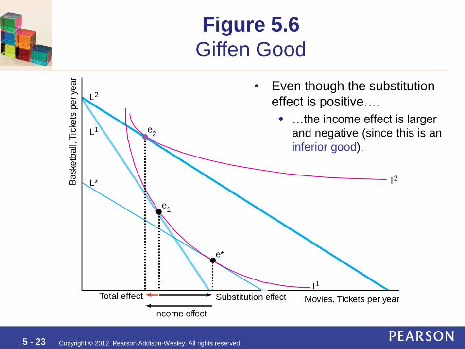
Figure 5.6

Giffen Good

When the price of movie tickets

decreases the budget constraint

rotates out…

allowing the consumer to

increase her utility.

Nevertheless, the total effect is negative. WHY?

Baske

tba

ll,T

icke

ts p

er

year

Movies, Tickets per year

L1

Total effect

L2

e1

e2

I1

I2


• Even though the substitution

effect is positive….

…the income effect is larger

and negative (since this is an

inferior good).

Bas k

etb

all,

Tic

k ets

perye

ar

Movies, Tickets per year

L1

L*

Income effect

Substitution effect

L2

e1

e2

e*

I1

I2

Total effect

Figure 5.6

Giffen Good

chapter 5 - benjamin a....

Documents