chapter 4 thermal effectiveness of a spiral plate heat...
TRANSCRIPT

55
CHAPTER 4
THERMAL EFFECTIVENESS OF A SPIRAL PLATE
HEAT EXCHANGER
4.1 INTRODUCTION
This chapter discusses the study of thermal effectiveness of the
spiral plate heat exchanger with liquid-liquid two-phase mixtures. Thermal
effectiveness is a measure of heat transfer efficiency of the exchanger.
It depends on the exchanger geometry, the properties of the hot and cold
fluids used, and on the range of operating conditions. Quantifying thermal
effectiveness of a heat exchanger is critical in designing the exchanger for
different applications. To determine the thermal effectiveness of a heat
exchanger, a geometric model of the exchanger has to be developed and a
model of heat transfer in the exchanger has to be developed. The model
development that follows is that of Bes and Roetzel (1993), which has been
used to study the thermal effectiveness of the spiral plate heat exchanger
involving heat transfer to liquid-liquid mixtures.
4.2 THERMAL EFFECTIVENESS
Thermal effectiveness measures the efficiency of heat transfer in
a heat exchanger. There are different definitions for the thermal
effectiveness, such as the ε-effectiveness and the P-effectiveness. Both are

56
usually studied as a function of the mean number of transfer units (NTU).
NTU measures the amount of heat to be transferred from the hot side to the
cold side for unit temperature difference in the fluid. Depending on the
length of the heat exchanger needed to accomplish this temperature
difference, the exchanger may be sized. The basic definition of thermal
effectiveness is the ratio of temperature difference accomplished in one of
the sides to the maximum span that can be accomplished. Thus, for the hot
side and the cold side, thermal effectiveness is defined as:
1c1h
1c2cc
1c1h
2h1hh
TT
TTP;
TT
TTP
−
−=
−
−= (4.1)
Thermal effectiveness is a function of NTU, heat capacity ratio,
and the flow arrangement (curvature). Further, the flow patterns in
two-phase flows can also significantly affect the thermal effectiveness of the
exchanger. It is of interest to evaluate whether a purely thermal theory for a
spiral plate heat exchanger such as the ones derived by Bes and Roetzel
(1993) and Martin (1992) is sufficient to reasonably capture the thermal
performance of the exchanger. In this chapter the thermal theory of Bes and
Roetzel (1993) is presented first, and expressions are derived for the thermal
effectiveness of the hot side and cold side. Using the experimental data and
the model equations, thermal effectiveness for hot and cold sides are
calculated and the trends analyzed. Thermal effectiveness is also calculated
from the inlet and outlet temperatures using the definition provided in
Equation 4.1. The predictions of the model are compared against
experimental data and the limitations of a purely thermal theory in
predicting the performance of a spiral plate heat exchanger with immiscible
liquid mixtures are examined.

57
4.3 THERMAL THEORY OF A SPIRAL PLATE HEAT
EXCHANGER
Bes and Roetzel (1993) have developed the thermal theory of
spiral plate heat exchangers wherein they have derived analytical
expressions for the LMTD correction factor and the temperature
effectiveness (P) of the exchanger. In what follows, the derivation of Bes
and Roetzel is presented. Direct mathematical manipulations are eschewed
as the original source is accessible.
4.3.1 Assumptions Involved
• The model applies only for the middle part of a spiral plate heat
exchanger, where heat is transferred to cold fluid from both walls.
Therefore the model works better for a spiral heat exchanger with
a large number of turns. In this study, the number of turns n = 60,
large enough for end-effects to be neglected.
• Flow is assumed to be countercurrent, and a correction factor F is
introduced for deviation from countercurrent flow.
• Flow is assumed to be steady.
• The exchanger geometry is assumed to be an Archimedean spiral.
This implies that the radius of the spiral increases, continuously
with the angle ϕ as:
( ) ,rb
r mm +ϕ−ϕπ
= (4.2)
58
where b - plate spacing, rm - minimum radius, and ϕm - angle at
which the minimum radius is achieved. Therefore, temperatures
may be expressed as a function of either radius or the angle.
• Fluids are assumed to be completely mixed in the radial and axial
directions within the flow channel. Thus in a cross-section chosen
at a fixed angle, the temperature changes step by step from
channel to channel.
• Hot fluid enters the exchanger in the centre of the apparatus and
cold fluid flows in at the outermost channel.
• Overall heat transfer coefficient U is constant throughout the
exchanger.
• There are no heat losses to the environment.
• Distance studs are not taken into account.
4.3.2 Thermal Theory
In this model, the mean temperature difference between the fluids
on both sides of a partition wall is tracked as a function of position in the
exchanger. To construct an Archimedean spiral plate exchanger, a double
slit is wound in a spiral fashion. Therefore, each “radius” corresponds to two
channels of rectangular cross sections. The ‘inner’ spiral is called the main
spiral, and hot fluid flows through it. The second spiral (made from the
‘outer’ slit) constitutes the side spiral, and the cold fluid flows
countercurrently through it. Thus, for each radius, two temperature
differences may be defined, as shown for an elementary wedge in

59
Figure 4.1. Both temperature differences are positive in the spiral plate heat
exchanger. Further, these differences of temperature depend upon each
other; however, for convenience they will be separately derived as two
different quantities and will later be combined with each other.
Figure 4.1 Temperature differences in an elementary wedge
of a spiral plate heat exchanger
4.3.3 Energy Balance Equations
Let the heat capacity of the hot fluid be Ch. For the part of the
channel between the radii r – 1 and r, the hot fluid flows in the counter
clockwise direction. Since ϕ is also measured counterclockwise, the flow
direction of the hot fluid is the positive direction of ϕ. This hot fluid loses
heat to the cold fluids in the channels between r − 1 and r − 2, and r and
r + 1. Denoting the channel between r – 1 and r as j, the above statement
may be rewritten as: the hot fluid in j loses heat to the cold fluid in j – 1 and
j + 1. Let the temperature of the hot fluid be denoted Th and that of the cold
fluid be denoted TC. In order to indicate the temperature dependence on the

60
position of the fluid in the exchanger, the temperature of the hot fluid in j is
denoted as ( ))21(rTh − , and that of the cold fluid in j + 1 is denoted as
( ))21(rTh + . Thus, the rate of change of heat transfer from the hot fluid in j
to the cold fluid in j + 1 with respect to the angle ϕ is given by:
+−
−=∆=+
2
1rT
2
1rThrwThAq ch1j,j (4.3)
Here the heat transfer area is given by A = (height of the
exchanger) × (arc length of the curved channel). This arc length is given at a
wedge by: ϕ= r1 Thus, the rate of change of heat transfer with respect to ϕ
results in the above expression, as a first approximation. Similar expressions
may be written for rates of heat transfer at other locations in the exchanger.
Performing an energy balance on the hot fluid at j whose temperature is
Th(r – ½), one obtains the equation
1j,j1j,j
hc
h qqd
2
1rd
C +− +=ϕ
−
− (4.4)
A similar energy balance for the cold fluid in j + 1 gives
2j,1j1j,j
c
c qqd
2
1rdT
C +++ +=ϕ
+
− (4.5)
It is convenient to change slightly the notation of temperatures.
The function of temperature
−
2
1rTh
and
+
2
1rTc
will be further denoted
as Th(r) and Tc(r), respectively. Instead of expressing the rate of change

61
with respect to the angle ϕ, one may convert this into the change with
respect to r. From Equation 4.2, we have drb
dπ
=ϕ .Thus, in the new
notations, Equations 4.4 and 4.5 become:
( ) ( ) ( )[ ]( ) ( ) ( )[ ]
−−−+
−=
π−
2rTrT1r
rTrTrkWb
dr
rdTC
ch
chhh
( ) ( ) ( )[ ]( ) ( ) ( )[ ]
−++
+−=
π−
rT2rT1r
rTrTrkWb
dr
rdTC
ch
chcc (4.6)
The boundary conditions are obtained from the inlet and outlet
temperatures of the hot and cold fluids, respectively in the centre of the
exchanger. These two equations contain two kinds of temperature
differences (see Figure 4.1):
1. Local temperature difference between the fluids flowing on both
sides of the main spiral: )r(T)r(T)r( ch −=∆
2. Local temperature difference between the fluids flowing on both
sides of the side spirals: )1r(T)1r(T)r( ch −−+=δ
Defining a mean heat capacity of the hot and cold fluids as
chCCC = , cross-sectional mean number of transfer units (NTU) as
C/hA2 cπ , the heat capacity ratio as c
h
C
CR = , and rearranging, the two
Equations in 4.6 may be recast as:

62
0)1r()1r()r(rdr
)r(dTR2 h =−ψδ−+∆ψ+
0)1r()1r()r(rdr
)r(dTR2 c =+ψδ++∆ψ+ (4.7)
To obtain the energy balance of the main and side spirals in terms
of the above defined local temperature differences, the derivatives have to be
converted to those in ∆(r) and δ(r). This involves algebraic manipulation of
the two Equations in 4.7, and expanding terms in Taylor’s series to second
derivative (Bes and Roetzel 1993). It turns out to be convenient to define a
new independent variable x which depends on r, as
rR
1R
2x
+ψ= (4.8)
The simplified final form of the two equations of ∆ and δ as a
function of x is:
( ) ( ) ( )[ ] ( )[ ]0
dx
xxdxxx
dx
xd=
δ−δ+∆µ−
∆
( ) ( ) ( )[ ] ( )[ ]0
dx
xxdxxx
dx
xd=
∆+δ+∆µ−
δ
(4.9)
The boundary conditions are: .)x( inlet);()x( ii δ=δ∆=∆
The Equations 4.9 are rearranged and solved by subtracting both equations
and integrating:
[ ] )(x)x()x(x)x()x( iiiii δ+∆−δ−∆=δ+∆−δ−∆ (4.10)
= constant

63
Since there are two variables ∆ and δ, another equation is needed
to find the final solution. This is obtained for the sum of the two variables.
Adding both Equations in 4.9 and replacing ( ) ( )xx δ−∆ using Equation 4.10
gives
( ))]x()x([x2
dx
)]x()x()[x1(d 2
δ+∆µ−δ+∆+
= [ ])(x iiiii δ+∆−δ−∆− (4.11)
Here an additional assumption is made that the radius rmin is small
enough to allow neglect of the term with ii rx ψ= in the last equation. This is
true for large n.
The solution of Equation 4.11 is readily obtainable. The final
function ( ) ( )xx δ+∆ is
( ) ( ) ( )( ) µ−
+δ+∆=δ+∆
12
iii
x1
Gxx (4.12)
where, µ−+= 12
ii )x1(G is a constant computed for the radius ri at
the inlet to the exchanger.
4.3.4 Effectiveness of Spiral Plate Heat Exchanger
The effectiveness Ph for spiral plate heat exchanger can be
calculated according to the general formula
i,ci,h
o,hi,h
hTT
TTP
−
−= (4.13)
64
This may also expressed as:
[ ][ ]NTU)1R(expR1
NTU)1R(exp1Ph
×−×−
×−−= (4.14)
Recasting the solution Equation 4.12 to obtain an expression for
thermal effectiveness gives
( )( ) ( )2
i
2
i
2
i
2
o
2
i
2
o
h
x1
x)1R(
x1
x1lnexpR1
x1
x1lnexp1
P
+
−+
+
+µ−
+
+µ−
= (4.15)
Here the term µ is given by
( ) ( )
( ) 2
h
2
CNNTU1R
R1RR1R2
−=
+−ψ
=µ (4.16)
where,
( ) ( )
( )A
ANTUNTUCN
AANTUR1RCN
cch
c
π+≅
π+=
(4.17)
This number is characteristic for spiral plate heat exchanger and
therefore Bes and Roetzel (1993) recognize CN as the dimensionless
criterion number for the countercurrent spiral heat exchanger.
The second term of exponent with ln function contains an
independent variable which can be expressed as follows:

65
( ) ( ) ( ) ( )2
i
2
i
2
o
2
i
2
o x1xx1x1x1 +−+=++
and
+
−+
=+
−2
i
2
2
i
2
i
2
o
x1
1n
11
CNx1
xx
For realistic heat capacity ratios (R) and small inlet radius, the
last term in the denominator ( ) ( )2
i
2
i x1x1R +− is negligible.
It is easy to notice that Equation 4.15 has the same structure as
Equation 4.14. The LMTD correction factor is obtained as
( )2
2
CN
CN1n
111ln
F
−++
= (4.18)
Therefore, for the hot side, thermal effectiveness, correcting
for deviation from countercurrent flow, is given by
( )[ ]( )[ ]FNTU1RexpR1
FNTU1Rexp1Ph
××−×−
××−−= (4.19)
Thermal effectiveness of the cold side is obtained from the
expression known in literature (Ramesh, K Shah 2006)
RPC
CPP h
c
hhc == (4.20)

66
4.3.5 Calculation from Experimental Data
From experimental data, the overall heat transfer coefficient may
be calculated as follows
( )LMTDTFUAQ ∆= (4.21)
Calculation of the heat transfer coefficient from Equation 4.19
requires the knowledge of LMTD correction factor whereas Equations 4.17
and 4.18 indicate that calculating F requires the knowledge of heat transfer
coefficient. Therefore an iterative procedure was setup and executed in
Microsoft Excel® to estimate the LMTD correction factor F, heat transfer
coefficient U, the number of transfer units NTU, and the temperature
effectiveness P of the exchanger for both the hot and the cold sides.
4.4 RESULTS AND DISCUSSION
The log mean temperature difference correction factors are very
close to unity for all octane-water, kerosene-water, dodecane-water,
diesel-water and nitrobenzene-water systems. The calculation data is
presented along with those of heat transfer coefficients in Chapter 5, in
Tables 5.3 to 5.28. The value of F being close to unity indicates that the flow
in the exchanger is predominantly countercurrent. Figures 4.2 through 4.34
show the thermal effectiveness of the spiral plate heat exchanger for the hot
and cold sides. It is seen that, as predicted by the model of Bes and Roetzel
(1993), the thermal effectiveness of both the hot and the cold sides increase
with increase in NTU. A typical plot of P-NTU of a spiral heat exchanger
for constant heat capacity ratio R and LMTD correction factor F is one of
asymptotic increase of P with respect to NTU, with the asymptote depending

67
on the heat capacity ratio and F. The experiments performed, however, have
been conducted for fixed hot fluid flow rates and varying cold fluid flow
rates. This implies that, as the cold fluid flow rate increases, its heat capacity
increases. Therefore, the heat capacity ratio R decreases continuously, even
as the NTU increases and the effectiveness increases. This preliminary study
has investigated the NTU range of practical relevance and the values of
thermal effectiveness range for the cold fluid, and the hot fluid is listed in
the Table 4.1.
Table 4.1 Ranges of NTU, thermal effectiveness of hot and cold fluid
System NTU Ph Pc
Min Max Min Max Min Max
Octane - Water 1.86 4.31 0.07 0.29 0.83 0.97
Kerosene - Water 0.28 3.93 0.07 0.59 0.23 0.97
Dodecane -Water 0.44 3.93 0.07 0.66 0.34 0.97
Diesel - Water 2.30 6.83 0.07 0.22 0.89 1.00
Nitrobenzene - Water 0.49 3.93 0.07 0.49 0.38 0.97
Thermal effectiveness may also be calculated from experimental
data on the inlet and outlet temperatures. These values, depicted in Figures
4.2 to 4.34 by the subscript exp, are also plotted as a function of NTU.
Further, the predictions of Bes and Roetzel are compared against the
experimental data. The following are the main observations:
• For the hot side, effectiveness increases monotonically with
NTU, and the model is able to capture this behavior qualitatively
as well as quantitatively. This is attributed to the turbulent flow

68
regime in the hot side, where the Reynolds Number is greater
than the critical Reynolds Number of the spiral exchanger.
• However, at low NTUs, the model overpredicts the effectiveness,
whereas at high NTUs, the model underpredicts the effectiveness.
The errors in these over/underpredictions are almost similar.
This brings out the limitation in using a purely thermal model to
predict heat transfer in heat exchangers.
• The results in the cold side are seemingly counterintuitive and
qualitatively different from experimental predictions. It is seen
that, while the experiments predict a decrease of the efficiency
with NTU, the model predicts the opposite. This is true for pure
cold fluids (water or organics) as well as the immiscible mixtures.
This discrepancy is explained with the water-water system as
follows: For a given quantity of heat transferred from the hot side
to the cold side, the more the heat capacity (i.e., the more the flow
rate), the smaller the temperature difference achieved.
This explains why thermal efficiency is poorer when heat transfer
coefficients are high. This behavior is not captured by the model.
Actually, in the hot side, the model performs admirably. Here, the
heat transfer coefficients (hh) decrease with increasing cold fluid
flow rate, and the thermal efficiency correspondingly increases.
The cold-side thermal efficiency is simply the product of heat
capacity ratio (R) and the hot-side thermal efficiency. As the
cold-side flow rate increases, R decreases, which should pull
down the value of cold-side efficiency. This happens, but
insufficiently, resulting in the preservation of the same trend in
the cold side as seen in hot side. This is best attributed to the fact

69
that the cold side has laminar flow while the hot side has
turbulent flow. Therefore, the reduction in R is insufficient to
reverse the trend. In other words, this is a limitation on the use of
a purely thermal model in the prediction of heat transfer in
laminar convection processes.
• An analysis of the thermal effectiveness in the case of liquid
mixtures reveals further insights. While the mixtures follow the
same trend as described above, the discrepancies fall under two
categories.
• In the case of water, octane and diesel, the model consistently
overpredicts the effectiveness. In all these systems, the Prandtl
Number is of the order of 5 to 7, which implies that heat transfer
is through both conduction and convection, though convection is
significant.
• In the next chapter, where a linear mixing rule is developed to
predict heat transfer to immiscible liquids, it is shown that
mixtures of these fluids obey what approaches stratified flow
pattern. Whether or not the flow pattern is stratified (or slug or
annular or three-layer), the non-negligible role of conduction
played in the system serves to lessen the importance of flow
patterns in the heat transfer behavior. This observation is further
validated by the results in the next chapter.
• In the case of kerosene, dodecane, and nitrobenzene, the model
underpredicts effectiveness in systems with higher organics
concentration, whereas as the amount of water increases, the
70
behavior tends to overprediction. For these systems, the Prandtl
Numbers are of the order of 17 to 26. In such systems, heat
transfer due to conduction is negligible. Here, the effects of flow
should be very significant in the laminar regime. As expected,
errors are much higher, and using weighted-average properties for
the mixtures tend to underpredict the actual heat transfer
effectiveness.
• In the next chapter, mixtures of these fluids are approximated to
flow in a oil-in-water or water-in-oil dispersion, and a linear
mixing rule is applied to predict their heat transfer coefficients.
This is to better capture the effect of flow on the heat transfer.
Even in the absence of a direct dependence on velocity, the heat
transfer coefficient predictions are reasonable, within an order of
magnitude, further validating the above observations.
• Bes and Roetzel model is able to predict that the thermal
effectiveness for kerosene, dodecane and nitrobenzene would be
lower than that of water, octane and diesel. However, the
magnitudes are significantly different, as explained above.
• The flow arrangement in the exchanger is not stream symmetric.
Hot fluid has much poorer thermal effectiveness than the cold
fluid. This is to be expected, because hot fluid flows much faster
(in turbulent regime) compared to the cold fluid (in laminar
regime).
• In the cold side, thermal effectiveness is highest for water, and
lowest for nitrobenzene system. Thermal efficiencies showed no

71
discernible trend respect to the amount of organic phase present
in the cold fluid. However, thermal effectiveness was higher for
lower-molecular weight organic phases such as octane and
kerosene, than the higher-molecular weight organic phases such
as dodecane and diesel. Polarity in the substance (as in
nitrobenzene) tended to decrease thermal effectiveness. The most
significant effect is that of the Prandtl Number, which effectively
determines whether heat transfer is by convection alone or if
conduction is to play an important role.
• Unlike the predictions of Bes and Roetzel (1992) and Burmeister
(2006) in their simulations, no maxima are observed for the
effectiveness for any composition of the two-phase mixture
within the range of Dean Number and Prandtl Number studied.
Burmeister has studied only the case of equal capacitances, and
Bes and Roetzel have examined cases of constant heat capacity
ratios. In the present work, on the one hand, NTU values are
smaller than those for which the maximum effectiveness is
observed by Burmeister. Also, in our measurements, the heat
capacity ratio decreases with increasing NTU.
• Further experiments are needed to study the quantitative
dependence of thermal effectiveness on carbon number and
composition of the organic phase, as well as the full functional
form of the dependence of thermal effectiveness on NTU for
liquid-liquid two-phase mixtures.

72
Figure 4.2 Thermal effectiveness with number of transfer units,
when pure cold fluids are used: From experiments
Figure 4.3 Thermal effectiveness with number of transfer units, when
pure cold fluids are used: From Bes and Roetzel model
0
0.2
0.4
0.6
0.8
1
1.2
0 2 4 6 8
Pc,e
xp
NTUc
Pure Water
Pure Octane
Pure Kerosene
Pure Dodecane
Pure Diesel
Pure Nitrobenzene
0
0.2
0.4
0.6
0.8
1
1.2
0 2 4 6 8
Pc,p
red
NTUc
Pure Water
Pure Octane
Pure Kerosene
Pure Dodecane
Pure Diesel
Pure Nitrobenzene

73
Figure 4.4 Thermal effectiveness comparison of model
vs. experiments when pure cold fluids are used
Figure 4.5 Thermal effectiveness with number of transfer units
in hot fluid for octane-water system: From experiments
0
0.1
0.2
0.3
0.4
0.5
0.6
0.7
0.8
0.9
1
0 0.1 0.2 0.3 0.4 0.5 0.6 0.7 0.8 0.9 1
Pc,e
xp
Pc,pred
Pure Water
Pure Octane
Pure Kerosene
Pure Dodecane
Pure Diesel
Pure Nitrobenzene
0.0
0.1
0.2
0.3
0.4
0.5
0.6
0.7
0.0 0.5 1.0 1.5
Tem
per
atu
re e
ffec
tiven
ess
Ph
, exp
Number of transfer units NTUh
Hot Fluid Pure Water
20% Octane
40% Octane
60% Octane
80% Octane
Pure Octane

74
Figure 4.6 Thermal effectiveness with number of transfer units
in hot fluid for octane-water system: From Bes and
Roetzel Model
Figure 4.7 Thermal effectiveness comparison of model
vs. experiments in hot fluid for octane-water system
0.05
0.10
0.15
0.20
0.25
0.30
0.35
0.15 0.65 1.15 1.65
Tem
per
atu
re e
ffec
tiven
ess
Ph
,pre
d
Number of transfer units NTUh
Hot Fluid Pure Water
20% Octane
40% Octane
60% Octane
80% Octane
Pure Octane
0.0
0.1
0.2
0.3
0.4
0.5
0.6
0.7
0.8
0.9
1.0
0.0 0.1 0.2 0.3 0.4 0.5 0.6 0.7 0.8 0.9 1.0
Tem
per
atu
re
effe
ctiv
enes
s P
h,
pre
d
Temperature effectiveness Ph, exp
Pure Water
20% Octane
40% Octane
60% Octane
80% Octane
Pure Octane

75
Figure 4.8 Thermal effectiveness with number of transfer units
in cold fluid for octane-water system: From experiments
Figure 4.9 Thermal effectiveness with number of transfer units
in cold fluid for octane-water system: From Bes and
Roetzel Model
0.0
0.2
0.4
0.6
0.8
1.0
0 1 2 3 4 5
Tem
per
atu
reef
fect
iven
ess
Pc,
exp
Number of transfer units NTUc
Cold FluidPure Water
20% Octane
40% Octane
60% Octane
80% Octane
Pure Octane
0.8
0.9
1.0
1.5 2.0 2.5 3.0 3.5 4.0
Tem
per
atu
re e
ffec
tiv
enes
s P
c,
pred
Number of transfer units NTUc
Cold Fluid
Pure Water
20% Octane
40% Octane
60% Octane
80% Octane
Pure Octane

76
Figure 4.10 Thermal effectiveness comparison of model
vs. experiments in cold fluid for octane-water system
Figure 4.11 Thermal effectiveness with number of transfer units in
hot fluid for kerosene-water system: From experiments
0.0
0.1
0.2
0.3
0.4
0.5
0.6
0.7
0.8
0.9
1.0
0.0 0.1 0.2 0.3 0.4 0.5 0.6 0.7 0.8 0.9 1.0
Tem
per
atu
re
effe
ctiv
enes
s P
c,
pre
d
Temperature effectiveness Pc, exp
Pure Water
20% Octane
40% Octane
60% Octane
80% Octane
Pure Octane
0.0
0.1
0.2
0.3
0.4
0.5
0.6
0.0 0.5 1.0 1.5
Tem
per
atu
re e
ffec
tiven
ess
Ph
, exp
Number of transfer units NTUh
Hot Fluid Pure Water
20% Kerosene
40% Kerosene
60% Kerosene
80% Kerosene
Pure Kerosene

77
Figure 4.12 Thermal effectiveness with number of transfer units
in hot fluid for kerosene-water system: From Bes and
Roetzel Model
Figure 4.13 Thermal effectiveness comparison of model
vs. experiments in hot fluid for kerosene-water system
0.05
0.15
0.25
0.35
0.45
0.55
0.65
0.15 0.65 1.15 1.65
Tem
per
atu
re e
ffec
tiv
enes
s P
h,
pred
Number of transfer units NTUh
Hot Fluid Pure Water
20 % Kerosene
40 % Kerosene60 % Kerosene
80 % Kerosene
Pure Kerosene
0.0
0.1
0.2
0.3
0.4
0.5
0.6
0.7
0.8
0.9
1.0
0.0 0.1 0.2 0.3 0.4 0.5 0.6 0.7 0.8 0.9 1.0
Tem
per
atu
re
effe
ctiv
enes
s P
h,
pre
d
Temperature effectiveness Ph, exp
Pure Water
20% Kerosene
40% Kerosene
60% Kerosene
80% Kerosene
Pure Kerosene

78
Figure 4.14 Thermal effectiveness with number of transfer units in
cold fluid for kerosene-water system: From experiments
Figure 4.15 Thermal effectiveness with number of transfer units
in cold fluid for kerosene-water system: From Bes and
Roetzel Model
0.0
0.2
0.4
0.6
0.8
1.0
1.2
0 2 4 6
Tem
per
atu
reef
fect
iven
ess
Pc, exp
Number of transfer units NTUc
Cold FluidPure Water
20% Kerosene
40% Kerosene
60% Kerosene
80% Kerosene
Pure Kerosene
0.0
0.2
0.4
0.6
0.8
1.0
0 1 2 3 4
Tem
per
atu
re e
ffec
tiven
ess
Pc,
pre
d
Number of transfer units NTUc
Cold Fluid
Pure Water
20 % Kerosene
40 % Kerosene
60 % Kerosene
80 % Kerosene
Pure Kerosene

79
Figure 4.16 Thermal effectiveness comparison of model
vs. experiments in cold fluid for kerosene-water system
Figure 4.17 Thermal effectiveness with number of transfer units in
hot fluid for dodecane-water system: From experiments
0.0
0.1
0.2
0.3
0.4
0.5
0.6
0.7
0.8
0.9
1.0
0.0 0.1 0.2 0.3 0.4 0.5 0.6 0.7 0.8 0.9 1.0
Tem
per
atu
re
effe
ctiv
enes
s P
c,
pred
Temperature effectiveness Pc, exp
Pure Water
20% Kerosene
40% Kerosene
60% Kerosene
80% Kerosene
Pure Kerosene
0.0
0.1
0.2
0.3
0.4
0.5
0.6
0.7
0.0 0.5 1.0 1.5 2.0
Tem
per
atu
re e
ffec
tiv
enes
s P
h,
exp
Number of transfer units NTUh
Hot Fluid Pure Water
20% Dodecane
40% Dodecane
60% Dodecane
80% Dodecane
Pure Dodecane

80
Figure 4.18 Thermal effectiveness with number of transfer units
in hot fluid for dodecane-water system: From Bes and
Roetzel Model
Figure 4.19 Thermal effectiveness comparison of model
vs. experiments in hot fluid for dodecane-water system
0.0
0.2
0.4
0.6
0.8
0.0 0.5 1.0 1.5 2.0
Tem
per
atu
re e
ffec
tiven
ess
Ph
, p
red
Number of transfer units NTUh
Hot Fluid Pure Water
20 % Dodecane
40 % Dodecane
60 % Dodecane
80 % Dodecane
Pure Dodecane
0.0
0.1
0.2
0.3
0.4
0.5
0.6
0.7
0.8
0.9
1.0
0.0 0.1 0.2 0.3 0.4 0.5 0.6 0.7 0.8 0.9 1.0
Tem
per
atu
re
effe
ctiv
enes
s P
h,
pre
d
Temperature effectiveness Ph, exp
Pure Water
20% Dodecane
40% Dodecane
60% Dodecane
80% Dodecane
Pure Dodecane

81
Figure 4.20 Thermal effectiveness with number of transfer units in
cold fluid for dodecane-water system: From experiments
Figure 4.21 Thermal effectiveness with number of transfer units
in cold fluid for dodecane-water system: From Bes
and Roetzel Model
0.2
0.4
0.6
0.8
1.0
0 2 4 6
Tem
per
atu
reef
fect
iven
ess
Pc,
exp
Number of transfer units NTUc
Cold Fluid Pure Water
20% Dodecane
40% Dodecane
60% Dodecanel
80% Dodecane
Pure Dodecane
0.3
0.4
0.5
0.6
0.7
0.8
0.9
1.0
0.0 2.0 4.0 6.0
Tem
per
atu
re e
ffec
tiven
ess
Pc,
pre
d
Number of transfer units NTUc
Cold Fluid Pure Water
20 % Dodecane
40 % Dodecane
60 % Dodecane
80 % Dodecane
Pure Dodecane

82
Figure 4.22 Thermal effectiveness comparison of model
vs. experiments in cold fluid for dodecane-water system
Figure 4.23 Thermal effectiveness with number of transfer units
in hot fluid for diesel-water system: From experiments
0.0
0.1
0.2
0.3
0.4
0.5
0.6
0.7
0.8
0.9
1.0
0.0 0.1 0.2 0.3 0.4 0.5 0.6 0.7 0.8 0.9 1.0
Tem
per
atu
re
effe
ctiv
enes
s P
c,
pre
d
Temperature effectiveness Pc, exp
Pure Water
20% Dodecane
40% Dodecane
60% Dodecane
80% Dodecane
Pure Dodecane
0.0
0.1
0.2
0.3
0.4
0.5
0.0 0.5 1.0 1.5
Tem
per
atu
re e
ffec
tiv
enes
s P
h,
exp
Number of transfer units NTUh
Hot Fluid Pure Water
20% Diesel
40% Diesel
60% Diesel
80% Diesel
Pure Diesel
83
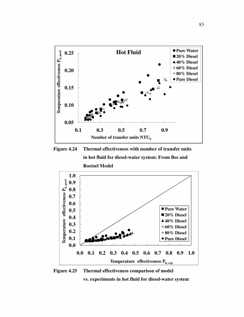
Figure 4.24 Thermal effectiveness with number of transfer units
in hot fluid for diesel-water system: From Bes and
Roetzel Model
Figure 4.25 Thermal effectiveness comparison of model
vs. experiments in hot fluid for diesel-water system
0.05
0.10
0.15
0.20
0.25
0.1 0.3 0.5 0.7 0.9
Tem
per
atu
re e
ffec
tiven
ess
Ph
, p
red
Number of transfer units NTUh
Hot Fluid Pure Water
20% Diesel
40% Diesel
60% Diesel
80% Diesel
Pure Diesel
0.0
0.1
0.2
0.3
0.4
0.5
0.6
0.7
0.8
0.9
1.0
0.0 0.1 0.2 0.3 0.4 0.5 0.6 0.7 0.8 0.9 1.0
Tem
per
atu
re
effe
ctiv
enes
s P
h,
pre
d
Temperature effectiveness Ph, exp
Pure Water
20% Diesel
40% Diesel
60% Diesel
80% Diesel
Pure Diesel

84
Figure 4.26 Thermal effectiveness with number of transfer units
in cold fluid for diesel-water system: From experiments
Figure 4.27 Thermal effectiveness with number of transfer units
in cold fluid for diesel-water system: From Bes and
Roetzel Model
0.0
0.2
0.4
0.6
0.8
1.0
0 2 4 6 8
Tem
per
atu
reef
fect
iven
ess
Pc, exp
Number of transfer units NTUc
Cold Fluid Pure Water
20% Diesel
40% Diesel
60% Diesel
80% Diesel
Pure Diesel
0.85
0.90
0.95
1.00
2 4 6 8
Tem
per
atu
re e
ffec
tiv
enes
s P
c,
pred
Number of transfer units NTUc
Cold Fluid Pure Water
20 % Diesel40 % Diesel60 % Diesel80% DieselPure Diesel

85
Figure 4.28 Thermal effectiveness comparison of model vs.
experiments in cold fluid for diesel-water system
Figure 4.29 Thermal effectiveness with number of transfer units
in hot fluid for nitrobenzene-water system: From
experiments
0.0
0.1
0.2
0.3
0.4
0.5
0.6
0.7
0.8
0.9
1.0
0.0 0.1 0.2 0.3 0.4 0.5 0.6 0.7 0.8 0.9 1.0
Tem
per
atu
re
effe
ctiv
enes
s P
c,
pred
Temperature effectiveness Pc, exp
Pure Water
20% Diesel
40% Diesel
60% Diesel
80% Diesel
Pure Diesel
0
0.1
0.2
0.3
0.4
0.5
0.6
0.7
0 0.5 1 1.5
Tem
per
atu
reef
fect
iven
ess
Ph
, ex
p
Number of transfer units NTUh
Hot Fluid Pure Water
20% Nitrobenzene
40% Nitrobenzene
60% Nitrobenzene
80% Nitrobenzene
Pure Nitrobenzene

86
Figure 4.30 Thermal effectiveness with number of transfer units
in hot fluid for nitrobenzene-water system: From Bes
and Roetzel Model
Figure 4.31 Thermal effectiveness comparison of model
vs. experiments in hot fluid for nitrobenzene-water
system
0.0
0.1
0.2
0.3
0.4
0.5
0.6
0.1 0.6 1.1 1.6
Tem
per
atu
re e
ffec
tiv
enes
s P
h,
pre
d
Number of transfer units NTUh
Hot Fluid Pure Water
20 % Nitrobenzene
40 % Nitrobenzene
60 % Nitrobenzene
80 % Nitrobenzene
Pure Nitrobenzene
0.0
0.1
0.2
0.3
0.4
0.5
0.6
0.7
0.8
0.9
1.0
0.0 0.1 0.2 0.3 0.4 0.5 0.6 0.7 0.8 0.9 1.0
Tem
per
atu
re
effe
ctiv
enes
s P
h,
pre
d
Temperature effectiveness Ph, exp
Pure Water
20% Nitrobenze
40% Nitrobenzene
60% Nitrobenzene
80% Nitrobenzene
Pure Nitrobenzene

87
Figure 4.32 Thermal effectiveness with number of transfer units
in cold fluid for nitrobenzene-water system: From
experiments
Figure 4.33 Thermal effectiveness with number of transfer units
in cold fluid for nitrobenzene-water system: From Bes
and Roetzel Model
0.0
0.2
0.4
0.6
0.8
1.0
0 2 4 6
Tem
per
atu
reef
fect
iven
ess
Pc,
exp
Number of transfer units NTUc
Cold Fluid Pure Water
20% Nitrobenzene
40% Nitrobenzene
60% Nitrobenzene
80% Nitrobenzene
Pure Nitrobenzene
0.3
0.4
0.5
0.6
0.7
0.8
0.9
1.0
0.0 1.0 2.0 3.0 4.0
Tem
per
atu
re e
ffec
tiv
enes
s P
c,
pre
d
Number of transfer units NTUc
Cold Fluid
Pure Water
20 % Nitrobenzene
40 % Nitrobenzene
60 % Nitrobenzene
80 % Nitrobenzene
Pure Nitrobenzene

88
Figure 4.34 Thermal effectiveness comparison of model
vs. experiments in cold fluid for nitrobenzene-water
system
0.0
0.1
0.2
0.3
0.4
0.5
0.6
0.7
0.8
0.9
1.0
0.0 0.1 0.2 0.3 0.4 0.5 0.6 0.7 0.8 0.9 1.0
Tem
per
atu
re
effe
ctiv
enes
s P
c,
pre
d
Temperature effectiveness Pc, exp
Pure Water
20% Nitrobenze
40% Nitrobenzene
60% Nitrobenzene
80% Nitrobenzene
Pure Nitrobenzene