111

CHAPTER 4

NON-DOMINATED SORTING GENETIC ALGORITHM-II

BASED ROUTE OPTIMIZATION

4.1 OVERVIEW OF NSGA-II

NSGA methodology discussed in Section 3.1 suffers from three

weaknesses: computational complexity, non-elitist approach and the need to

specify a sharing parameter. An improved version of NSGA known as

NSGA-II, which resolved the above problems and uses elitism to create a

diverse Pareto-optimal front, has been subsequently presented (Deb et al

2002). The main features of NSGA-II are low computational complexity,

parameter less diversity preservation, elitism and real valued representation.

NSGA-II implements elitism for multi-objective search, using an

elitism-preserving approach. Elitism is introduced by storing all non-

dominated solutions discovered so far, beginning from the initial population.

Elitism enhances the convergence properties towards the Pareto-optimal set.

A parameter-less diversity preservation mechanism is adopted. Diversity and

spread of solutions are guaranteed without the use of sharing parameters,

since NSGA-II adopts a suitable parameter-less niching approach. It uses the

crowding distance, which estimates the density of solutions in the objective

space, and the crowded comparison operator, which guides the selection

process towards a uniformly spread Pareto-frontier (Basu 2008).

112

In NSGA-II, the offspring population Qt is first created by using the

parent population P t, of size Z. However, instead of finding the non-

dominated front of Qt, the two populations are combined together to form Rt

of size 2Z. Then, non-dominated sorting is used to classify the entire

population Rt. The new population is filled by solutions of different non-

dominated fronts, one at a time. The filling starts with the best non-dominated

front and continues with solutions of the second non-dominated front,

followed by the third, and so on. Since the overall population size of Rt is 2Z,

not all fronts may be accommodated in Z slots available in the new

population. All fronts which could not be accommodated are simply deleted.

When the last allowed front is being considered, there may exist more

solutions in the last front than the remaining slots in the new population.

Instead of arbitrarily discarding some members from the last front, a niching

strategy is used to choose the members from the last front, which reside in the

least crowded region in the front. The algorithm ensures that niching will

choose a diverse set of solutions from this set. When the entire population

converges to the Pareto-optimal front, the continuation of this algorithm will

ensure a better spread among the solutions. The schematic representation of

NSGA-II procedure is shown in Figure 4.1.

Figure 4.1 Schematic of the NSGA-II procedure

P t

Qt

F1

F2

F3

P t+1

Non-dominated

sorting

Crowding

distance sorting

Rejected

Rt

113

4.2 IMPLEMENTATION OF NSGA-II IN ROUTING PROBLEM

A general NSGA-II procedure to be implemented in routing

problem is presented in the following steps:

Step 1: Create a random parent population, P t of size Z.

Step 2: Sort the random parent population based on non-domination.

Step 3: For each non-dominated solution, assign a fitness (rank) equal to its

non-domination level (1 is the best level, 2 is the next best level,

and so on).

Step 4: Create an offspring population, Qt of size Z using binary

tournament selection, recombination, and mutation operators.

Step 5: From the first generation onwards, creation of each new generation

constitutes the following steps:

a) Create the mating pool Rt, of size 2Z by combining the

parent population, Pt and the offspring population, Qt.

b) Sort the combined population, Rt, according to the fast

non-dominated sorting procedure to identify all non-

dominated fronts (Fr1, Fr2, . . . ,Frl).

c) Generate the new parent population, P t+ 1 of size Z by

adding non-dominated solutions starting from the first ranked

non-dominated front, Fr1. When the total non-dominated

solutions exceed the population size Z, reject some of the

lower ranked non-dominated solutions. This is achieved

through a sorting procedure which is done according to the

crowded comparison operator based on the crowding distance.

d) Perform the selection, crossover and mutation operations

on the newly generated parent population, P t+1 to create the

new offspring population, Qt+1 of size Z.

Step 6: Repeat Step 5 until the maximum number of iterations is reached.

114

The flowchart for NSGA-II is shown in Figure 4.2.

Figure 4.2 Flowchart of NSGA-II

Start

No

Selection

Rank population

Evaluation of objective

functions

Evaluation of objective

functions

Stopping criteria met?

Report solution and

stop

Initialize population

(size = Z)

Combine parent and offspring

populations, rank population

Select Z individuals

Yes

Crossover

Mutation

115

4.3 NSGA-II BASED UNICAST ROUTING

4.3.1 Population Initialization

The priority based encoding scheme that is explained in

Section 3.3.1.2 is used to create an initial population P t, of size Z.

4.3.2 Identification of Non-dominated Set

Kung et al’s efficient method is used to identify the non-dominated

solution present in the initial population. Since this method has lesser number

of computations, this method is suitable to find the non-dominated solutions

in the initial population. A detailed explanation about Kung et al’s method is

given in Section 3.3.2.1.

4.3.3 Fitness Assignment

In single-objective optimization, elites are easier to be identified.

They are the better solutions in a population pool. The best elite is the

solution with the best objective value. Since there are many objective

functions in MOO, it is not straightforward, like that in the single objective

case to identify the elites. In such situations, the non-domination ranking is

used. Thus, each member is assigned a fitness (rank) equal to its non-

domination rank, 1 is the best level, 2 is the next best level, and so on.

4.3.3.1 Fast non-dominated sorting approach

NSGA-II uses an explicit diversity-preserving mechanism. In order

to sort a population of size Z according to the level of non-domination, each

solution must be compared with every other solution in the population to find

if it is dominated. First, for each solution, two entities are calculated:

1) y, the number of solutions which dominate the solution y

2) y, the set of solutions, that solution y dominates.

116

The points which have y = 0 is first identified, and placed in a list

Fr1. Fr1 is called the current front. Now, for each solution in the current front,

each member in its set y is visited and its count is reduced by one. In doing

so, for any member, if the count becomes zero, it is put in a separate list H.

When all members of the current front had been checked, the members in the

list Fr1 is declared as members of the first front. Then this process is continued

using the newly identified front H as the current front. The fast non-

dominated sorting procedure which when applied on a population Z returns a

list of the non-dominated fronts Fr. Once the non-dominated sorting is over,

the new population is filled by solutions of different non-dominated fronts,

one at a time. The filling starts with the best non-dominated front and

continues with solutions of the second non-dominated front, followed by the

third and so on. Since overall population is 2Z in Rt, all fronts cannot be

accommodated in Z slots in the new population. All fronts which could not be

accommodated are simply deleted.

4.3.5 Fast Crowded Distance Estimation Procedure

To get an estimate of the density of solutions surrounding a

particular solution in the population, the average distance of two solutions on

either side of a particular solution i along each of the objectives is calculated.

This quantity serves as an estimate of the perimeter of the cuboid formed by

using the nearest neighbours as the vertices. This is called crowding distance,

idistance. In Figure 4.3, the crowding distance of ith

solution in its front (marked

with solid circles) is the average side length of the cuboid (shown by box).

The crowding distance computation requires sorting the population according

to each objective function value in ascending order of magnitude. Thereafter,

for each objective function, the boundary populations are assigned an infinite

distance value. All other intermediate populations are assigned a distance

equal to the absolute normalized difference in the function values of two

117

adjacent populations. This calculation is continued with other objective

functions. The overall crowding distance value is calculated as the sum of

individual distance values corresponding to each objective. Each objective

function is normalized before calculating the crowding distance. The

crowding distance calculation is shown in Figure 4.3.

Figure 4.3 The Crowding distance calculation

The algorithm used to calculate the crowding distance of each point

in the set Fu is given below:

Step 1: The number of solutions in Front Fr is called as v. For each solution

in the set, first assign crowding distance as 0.

Step 2: For each objective function fm, m =1, 2,..., M, sort the set in worse

order of fm or, find the sorted indices vector, Fm = sort (fm, >).

Step 3: For m = 1, 2,..., M, assign a large distance to the boundary

solutions, 1 is the first solution in the front and l is the last solution

in the front, or ml

mFF

dd1

, and for all other solutions j = 2 to (l

– 1), assign:

minmax

)()( 11

1

mm

F

m

F

m

FF ff

ffdd

mv

mv

mv

mv

(4.1)

f2

f1

i + 1

i – 1

i

0

l

118

)( 1m

vF

mf is the m

th objective function value of the (v+1)

th individual in

the set Fr

)( 1m

vF

mf is the m

th objective function value of the (v–1)

th individual in

the set Fr

max

mf is the population-maximum of the mth

objective function

min

mf is the population-minimum of the mth

objective function.

NSGA-II performs a non-dominated sorting of the combined parent

and offspring population. Elitism is introduced by maintaining the best non-

dominated solutions in fronts until all Z population slots are filled. A crowded

distance-based niching strategy is used to find solutions from the last front

that are to be carried over to the next generation.

4.3.6 Crowded-comparison Operator

The crowded-comparison operator guides the selection process at

various stages of the algorithm towards a uniformly spread out Pareto-optimal

front. Every individual in the population has two attributes: non-domination

rank, irank and crowding distance, idistance. A partial order can be defined as

if (irank < jrank ) or ((irank = jrank ) and (idistance = jdistance )) (4.2)

Between two populations with differing non-domination ranks, the

population with the lower rank is preferred. If both populations pertain to the

same front, then the population with larger crowding distance is preferred.

4.3.7 Tournament Selection

Selection mechanism’s role is important in improving the average

quality of the population by passing the high quality chromosomes to the next

119

generation. The individual with the lowest front number is selected if the two

individuals are from different fronts. The individual with the highest

crowding distance is selected if they are from the same front. A higher fitness

is assigned to individuals located on a sparsely populated part of the front. In

each iteration, the existing Z parents generate Z new offspring. Both parents

and offspring compete with each other for inclusion in the next iteration.

4.3.8 Crossover

PMX scheme is used for crossover operation. The reason for doing

so is given in Section 3.3.4.2 of the previous chapter.

4.3.9 Mutation

Mutation is done by single point mutation method, where the

mutation point is selected at random and a random number is replaced at that

particular point.

4.3.10 Stopping Criteria

If the number of iterations exceeds its maximum preset limit of 100

then the algorithm stops.

4.4 EXPERIMENTS AND RESULTS

In order to investigate the capability of NSGA-II algorithm in

solving the QoS routing problem, unicast routing was considered at first,

where the same 20 node sample network shown in Figure 3.3 is taken up for

study. Initially, NSGA-II was applied to minimize two objective functions

cost and delay simultaneously. The algorithm was implemented and 100

simulation runs were conducted to test the effectiveness of the routing

algorithm. For all the runs, the sender was always the first node and the

120

receiver was the twentieth node since that would give the largest number of

possible paths in the network. Table 4.1 shows the set of control parameters

selected after conducting several experiments.

Table 4.1 Control parameters selected for NSGA-II algorithm

Parameter Set value

Population size, Z 30

Number of generations 100

Cross over probability Pc 0.8

Mutation probability Pm 0.1

4.4.1 Pareto-optimal Set

For the sample 20 node network problem shown in Figure 3.3,

NSGA-II was also able to find the 23 non-dominated solutions shown in

Table 3.1, in a single run. This Pareto-optimal set was obtained by taking only

the two objectives cost and delay. The minimum value of cost returned by

NSGA-II was 158 and the minimum delay was 120 seconds.

Further the algorithm was implemented on various network

topologies and various network sizes to test the performance in finding the

Pareto-optimal solutions, the RO, the ET and the scalability. As done in the

previous chapter, the entire group of different networks was split into smaller

size networks (20 to 100 nodes) and larger size networks (200 to 1000 nodes).

The ranges of cost, delay and bandwidth of the links were assumed to be the

same values as in Chapter 3. After performing 100 simulation runs, the best

results achieved by NSGA-II were recorded and they are shown in Tables 4.2

and 4.3 respectively for smaller and larger size networks.

121

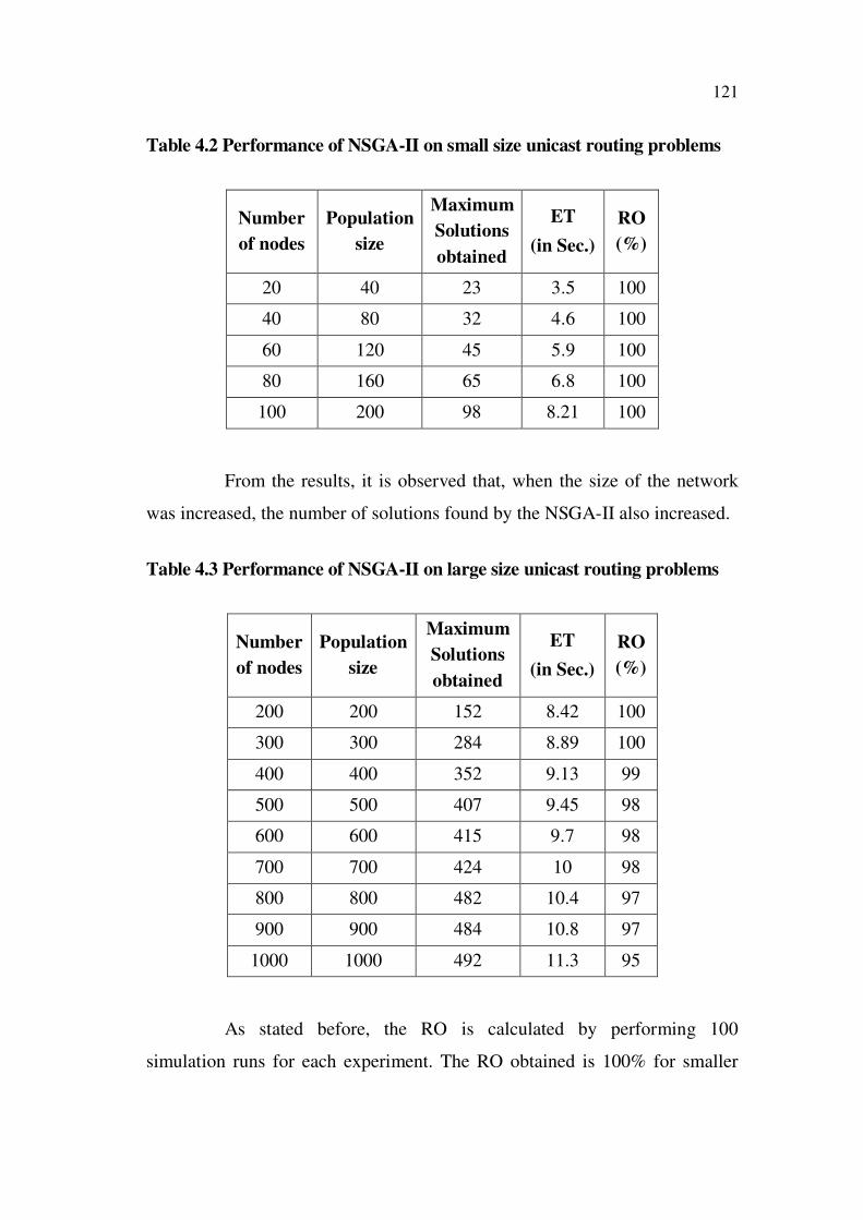
Table 4.2 Performance of NSGA-II on small size unicast routing problems

Number

of nodes

Population

size

Maximum

Solutions

obtained

ET

(in Sec.)

RO

(%)

20 40 23 3.5 100

40 80 32 4.6 100

60 120 45 5.9 100

80 160 65 6.8 100

100 200 98 8.21 100

From the results, it is observed that, when the size of the network

was increased, the number of solutions found by the NSGA-II also increased.

Table 4.3 Performance of NSGA-II on large size unicast routing problems

Number

of nodes

Population

size

Maximum

Solutions

obtained

ET

(in Sec.)

RO

(%)

200 200 152 8.42 100

300 300 284 8.89 100

400 400 352 9.13 99

500 500 407 9.45 98

600 600 415 9.7 98

700 700 424 10 98

800 800 482 10.4 97

900 900 484 10.8 97

1000 1000 492 11.3 95

As stated before, the RO is calculated by performing 100

simulation runs for each experiment. The RO obtained is 100% for smaller

122

size networks that could be noted from Table 4.2. Even up to 300 nodes, the

RO obtained by NSGA –II was 100%, i.e. in all the simulation runs carried

out, the Pareto-optimal solutions were obtained. When the network size

becomes larger, the RO tends to get reduced. Obviously, for the 1000 node

network case, it is only 95%. Figure 4.4 shows the variation of RO with

increase in number of nodes.

Figure 4.4 RO by NSGA-II in large size unicast routing problems

Tables 4.2 and 4.3 give the ET needed by the CPU to identify the

Pareto-optimal set. Its variations against the number of nodes are presented in

Figures 4.5 and 4.6.

200 400 600 800 100092

93

94

95

96

97

98

99

100

101

Number of nodes

Ro

ute

Op

tim

ali

ty

NSGA-II

123

Figure 4.5 ET by NSGA-II in small size unicast routing problems

Figure 4.6 ET by NSGA-II in large size unicast routing problems

200 400 600 800 10005

6

7

8

9

10

11

12

13

14

Number of nodes

Exec

uti

on

Tim

e (s

eco

nd

s)

NSGA-II

20 40 60 80 100 1200

2

4

6

8

10

Number of nodes

Exec

uti

on

Tim

e (s

econ

ds)

NSGA-II

124

When the number of nodes in the network was 20, the ET was 3.5

seconds and when the size of the network was increased, the ET also

increased. For a 100 node network the ET was found to be 8.21 seconds.

When increasing the number the nodes further, it was observed that the ET

also increased. When the maximum network size was taken to be 1000, the

maximum ET was found to be 11.3 seconds. The ET for various network

sizes is plotted in Figure 4.5 and Figure 4.6.

The maximum number of trade-off solutions obtained by the

NSGA-II was found to be 98 when the size of the network had 100 nodes. In

the case of 800 node network, the number of solutions obtained by NSGA-II

is 482 and the number of solutions obtained by NSGA for the same 800 node

network is 475, thus outperforming the latter. For 1000 node network case

too, more number of solutions were identified by NSGA-II, than NSGA.

It could be observed that the improved version of NSGA is a

superior multi-objective optimization tool than NSGA, as far as the quality of

solutions and execution time is concerned. The increase in number of

solutions with respect to the increase in number of nodes is shown in Figure 4.7.

Figure 4.7 Solutions of unicast routing problem identified by NSGA-II

0

100

200

300

400

500

600

Nu

mb

er o

f S

olu

tion

s

Number of nodes

NSGA-II

125

4.5 NSGA-II BASED MULTICAST ROUTING

4.5.1 Population Initialization, Crossover and Mutation

Similar to unicast routing, PBE technique is used here for

population generation. Since flow crossover method is found to be better

when compared to tree crossover, it is used in NSGA-II. Mutation is done by

single point mutation method.

4.6 EXPERIMENTS AND RESULTS

This section analyzes the performance of the NSGA-II in terms of

number of non-dominated solutions identified, the RO, the ET and the

scalability in multicast routing problems. The same simulation environment

was maintained with MATLAB 7.4, software package. The range of cost was

varied from 10 to 250 and the range of delay from 5 to 300. All links were

assumed to have 1.5 Mbps of bandwidth capacity. Control parameters such as

crossover probability and mutation probability were chosen as 0.8 and 0.1

respectively. The multicast group size was fixed as 5 and the maximum

number of iterations was set as 100. Each experiment was conducted 100

times and the average ET and RO are recorded in Table 4.4 and Table 4.5.

Table 4.4 Performance of NSGA-II on small size multicast routing problems

Number

of nodes

Maximum

Solutions

obtained

ET

(in Sec.)

RO

(%)

20 32 9.7 100

40 41 11.4 100

60 53 13.9 100

80 65 15.3 100

100 74 16.2 99

126

Figure 4.8 RO by NSGA-II in small size multicast routing problems

From the results that are tabulated in Table 4.4, it is clear that the

RO obtained by NSGA-II was 100% when the size of the network was varied

from 20 to 80 nodes.

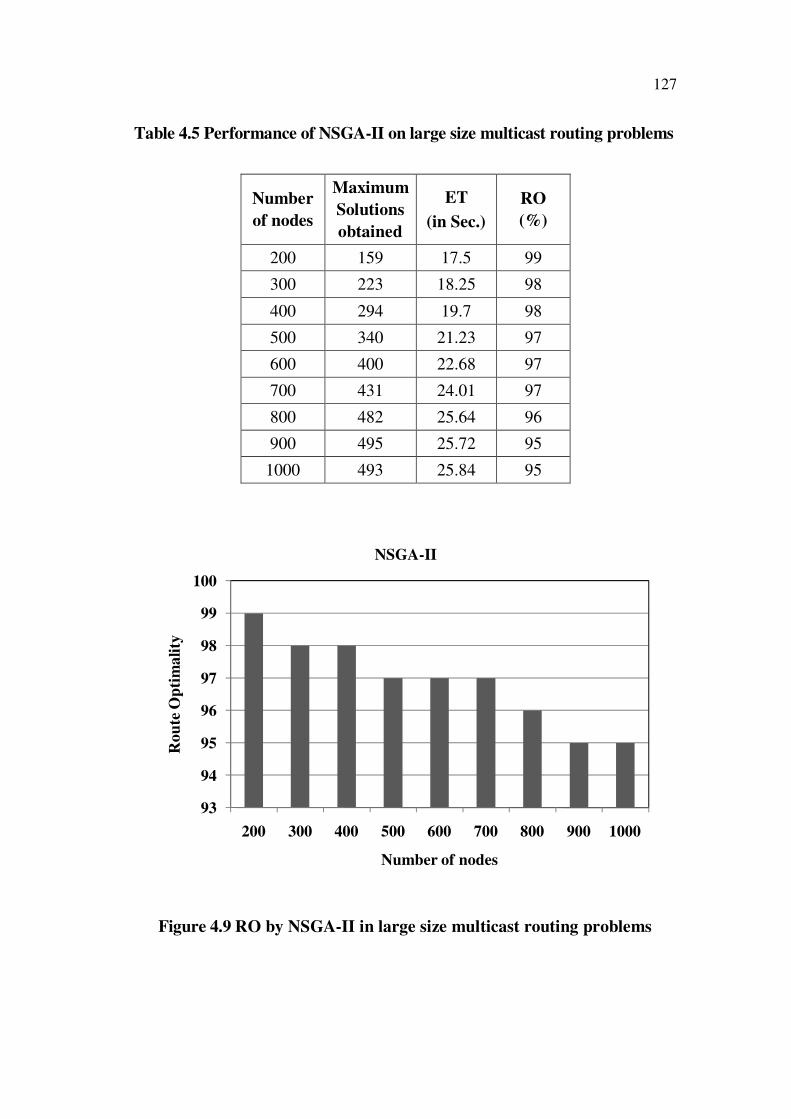
When the number of nodes in the network was increased from 100

to 1000 the RO decreased from 99% to 95%. The worst route optimality

obtained was 95% when the size of the network had maximum number of

nodes considered in this thesis. The variation of RO with increase in number

of nodes is shown in Figure 4.8 and Figure 4.9 for the two groups, smaller and

larger sizes separately.

The ET required by the NSGA-II to obtain the Pareto-optimal set

when the number of nodes in the network was varied from 20 to 100 is given

in Table 4.4. Figure 4.10 shows the ET required by the NSGA-II for various

network sizes. When the number of nodes in the network was increased above

100 up to 1000 nodes the ET required by the NSGA-II to obtain the Pareto-

optimal set is shown in Table 4.5. When the number of nodes in the network

was 20, the ET was 9.7 seconds only.

98.5

99

99.5

100

20 40 60 80 100

Ro

ute

Op

tim

ali

ty

Number of nodes

NSGA-II

127

Table 4.5 Performance of NSGA-II on large size multicast routing problems

Number

of nodes

Maximum

Solutions

obtained

ET

(in Sec.)

RO

(%)

200 159 17.5 99

300 223 18.25 98

400 294 19.7 98

500 340 21.23 97

600 400 22.68 97

700 431 24.01 97

800 482 25.64 96

900 495 25.72 95

1000 493 25.84 95

Figure 4.9 RO by NSGA-II in large size multicast routing problems

93

94

95

96

97

98

99

100

200 300 400 500 600 700 800 900 1000

Ro

ute

Op

tim

ali

ty

Number of nodes

NSGA-II

128

Figure 4.10 ET by NSGA-II in small size multicast routing problems

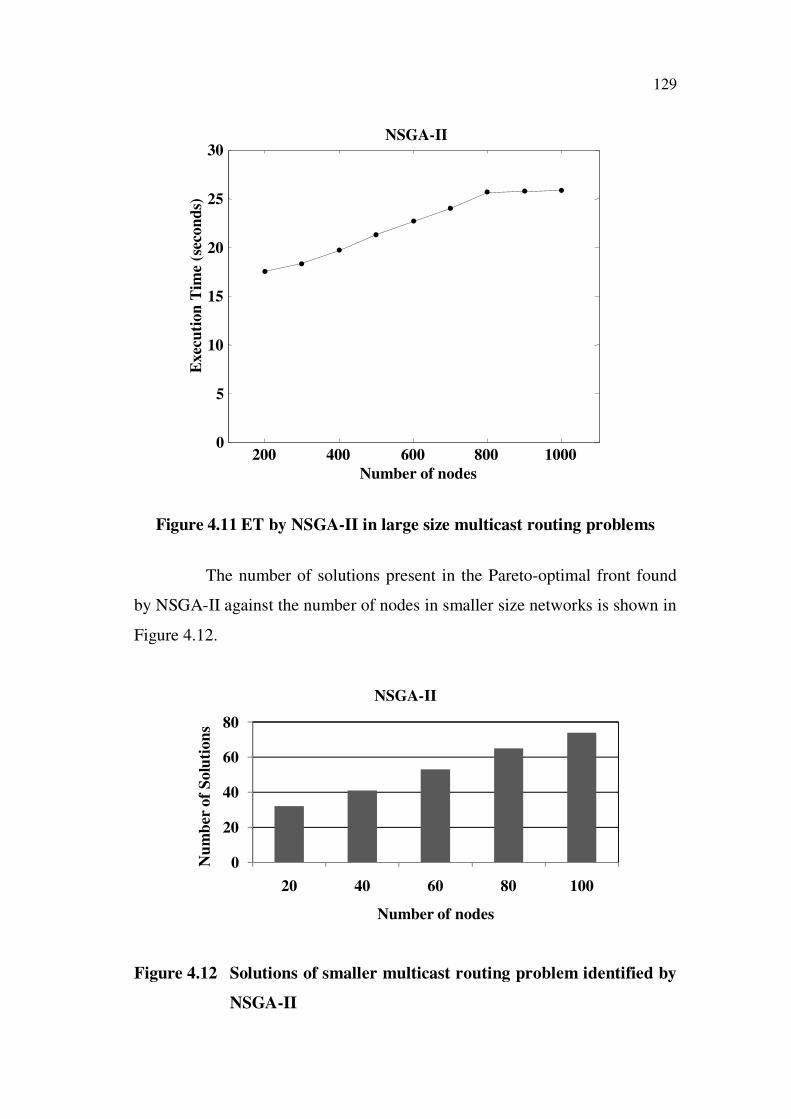
The ET for various network sizes when the number of nodes in the

network was varied from 20 to 100 is plotted in Figure 4.10. Similarly, the ET

for various network sizes when the number of nodes in the network was

varied from 100 to 1000 is plotted in Figure 4.11. From Figures 4.10 and

4.11, it is observed that when the number of nodes in the network is

increased, the ET increases almost exponentially. The maximum ET was

25.84 seconds when the number of nodes in the network was made 1000.

When the number of nodes in the network was equal to 20 in

multicast transmission, the number of Pareto-optimal solutions obtained by

NSGA-II is 32, and when the size of the network was increased till 100 nodes,

the maximum number of solutions identified by NSGA-II also varied till 74

non-dominated solutions, which is evident from Table 4.4.

20 40 60 80 100 1200

5

10

15

20

Number of nodes

Exec

uti

on

Tim

e(s

eco

nd

s)

NSGA-II

129

Figure 4.11 ET by NSGA-II in large size multicast routing problems

The number of solutions present in the Pareto-optimal front found

by NSGA-II against the number of nodes in smaller size networks is shown in

Figure 4.12.

Figure 4.12 Solutions of smaller multicast routing problem identified by

NSGA-II

0

20

40

60

80

20 40 60 80 100

Nu

mb

er o

f S

olu

tio

ns

Number of nodes

NSGA-II

200 400 600 800 10000

5

10

15

20

25

30

Number of nodes

Exec

uti

on

Tim

e (s

econ

ds)

NSGA-II

130

The experiment was repeated by increasing the number of nodes

from 200 to 1000 and the number of solutions obtained by the NSGA-II is

shown in Table 4.5.

Figure 4.13 Solutions of larger multicast routing problem identified by

NSGA-II

4.6.1 Execution Time as a Function of Group Size

In this section the scalability of the algorithm is investigated when

the number of destination nodes (group size) in the network was changed.

When the group size is increased, it increases the traffic in the network routes.

The number of nodes in the network was varied from 20 to 1000 and the

multicast group size was varied as 25%, 35%, 45% and 50% of the total

network size. This experiment also intended to study the performance of the

algorithm in terms of execution time when the destination group sizes were

increased.

The ET required by the NSGA-II to obtain the Pareto-optimal

solutions for various network sizes is given in Table 4.6. When the size of the

network and the size of the multicast group were increased, the ET of NSGA-

II also increased.

0

100

200

300

400

500

600

200 300 400 500 600 700 800 900 1000

Nu

mb

er o

f S

olu

tio

ns

Number of nodes

NSGA-II

131

Table 4.6 Execution Time variation of NSGA-II with different group size

problems

Number

of nodes

ET (in sec.) for Group size

25% 35% 45% 50%

100 16.2 18.6 19.7 22.1

200 17.01 19.4 20.1 23.2

300 18.25 20.21 21.5 25.2

400 19.68 21.43 23.2 27.3

500 21.23 22.65 24.8 28.9

600 22.89 23.78 26.1 29.5

700 23.52 24.36 28.2 33.3

800 25.64 24.98 30.4 35.7

900 29.82 28.1 34.3 39.1

1000 33.48 32.2 38.2 43.8

Figure 4.14 Execution Time variation of NSGA-II with different group

size problems

0 200 400 600 800 1000

10

20

30

40

50

60

Number of nodes

Ex

ecu

tio

n t

ime (

seco

nd

s)

NSGA-II

Group size 25%

Group size 35%

Group size 45%

Group size 50%

132

The Figure 4.14 shows the ET required by NSGA-II to obtain the

Pareto-optimal solutions when the number of nodes in the network and the

multicast group size were also increased. When the ET required by NSGA-II

to find the optimal set is compared with the ET required by NSGA, it is found

that NSGA-II requires lesser time.

4.7 CONCLUSION

In this chapter, NSGA-II approach has been proposed which

optimizes the same four objectives cost, delay, hop count and MLU of QoS

routing problem with flow constraints. The problem has been simulated

separately for unicast transmission and multicast transmission. Using the

control parameters determined in the previous chapter simulation experiments

were conducted to investigate the capability of the algorithm’s problem

solving qualities in terms of quality of solution, route optimality, execution

time and scalability. Numerous experiments were conducted to obtain

sufficient results to compare each other with other MOEAs studied in this

thesis.