chapter 4 measures of variability distribute · introduces measures of variability, which are...

ww104

Measures of Variability

CHAPTER

4

Chapter Outline4.1 An Example From the Research: How Many “Sometimes” in an “Always”?

4.2 Understanding Variability

4.3 The Range

• Strengths and weaknesses of the range

4.4 The Interquartile Range

• Strengths and weaknesses of the interquartile range

4.5 The Variance (s2)

• Definitional formula for the variance

• Computational formula for the variance

• Why not use the absolute value of the deviation in calculating the variance?

• Why divide by N – 1 rather than N in calculating the variance?

4.6 The Standard Deviation (s)

• Definitional formula for the standard deviation

• Computational formula for the standard deviation

4.7 Measures of Variability for Populations

• The population variance (σ2)• The population standard

deviation (σ)

Chapter 3 introduced descriptive statistics, the purpose of which is to numerically describe or summarize data for a variable. As we learned in Chapter 3, a set of data is often described in terms of the most typical, common, or frequently occurring score by using a measure of central tendency such as the mode, median, or mean. Measures of central ten-dency numerically describe two aspects of a distribution of scores, modality and symmetry, based on what the scores have in common with each other. However, researchers also describe the amount of differences among the scores of a variable in analyzing and reporting their data. This chapter introduces measures of variability, which are designed to rep-resent the amount of differences in a distribution of data. In this chapter, we will present and evaluate different measures of variability in terms of their relative strengths and weak-nesses. As in the previous chapters, our presentation will depend heavily on the findings and analysis from a published research study.

4.1 An Example From the Research: How Many “Sometimes” in an “Always”?

Throughout our daily lives, we are constantly asked to fill out questionnaires and surveys. Restaurants ask us to evaluate the quality of the food and service they provide; companies want to know how often we shop online; political organizations are interested in knowing what we think about our elected offi-cials. In responding to these types of scenarios, we are often asked to describe our feelings, behaviors, or beliefs by choos-ing among comparative terms such as excellent, good, or poor. To what degree do words such as these have the same mean-ing for different people? Researchers who collect data using questionnaires are concerned about the clarity of the words

Copyright ©2016 by SAGE Publications, Inc. This work may not be reproduced or distributed in any form or by any means without express written permission of the publisher.

Do not

copy

, pos

t, or d

istrib

ute

105Chapter 4 | Measures of Variability

they use. If research participants do not agree about the mean-ing of key terms and phrases, it is difficult to combine or com-pare their responses. The following example demonstrates how important it is to understand and address these differences when research is conducted with people of different backgrounds, cul-tures, or languages.

As members of an international research team, two British researchers, Suzanne Skevington and Christine Tucker, con-ducted a study assessing differences in interpretation of labels for questionnaire items measuring the frequency of health-related behaviors, such as, “How often do you suffer pain?” (Skevington & Tucker, 1999). As a part of their study, they examined how British people define frequency-related terms such as seldom, usually, and rarely. To this end, the researchers assigned numeric values to participants’ evaluation of these words in order to mea-sure the degree to which people differ in their interpretation of these words.

In their study, Skevington and Tucker (1999) presented 20 British adults a series of fre-quency-related words. For each word, they included a line 100 millimeters (about 4 inches) in length. At opposite ends of the line were attached the labels Never and Always, representing the lowest and highest possible values for frequency. After reading each word, participants were asked to place an X on the point in the line that in their opinion best represented the frequency of the word, relative to the end points of Never (0%) and Always (100%). An example of their methodology is provided in Figure 4.1.

After the participants had completed their responses, the researchers used a ruler to measure, for each word, the distance from the word Never to the “X” provided by the participant. This distance, which was measured in millimeters, represented the perceived “frequency” of the word. For example, in Figure 4.1, the X for the word sometimes is in the exact middle of the line; consequently, this word is given a frequency rating of 50% because it is 50 mm from the left end. In this study, the variable, which we will call “frequency rating,” had possible values ranging from 0 to 100.

In this example, we will focus on the study’s findings regarding the word sometimes. The frequency ratings for the word sometimes for the 20 participants are listed in Table 4.1(a). Table 4.1(b) organizes the raw data into a grouped frequency distribution table, and Figure 4.2 illustrates the distribution using a frequency polygon. A frequency polygon is used for this variable (rather than a histogram or pie chart) because the variable “frequency rating” is measured at the ratio level of measurement, with the value of 0 representing the complete absence of distance from the left end of the 100-mm line.

As was discussed in Chapter 3, the data for a variable can be summarized using a measure of central tendency. Using Formula 3-3 from Chapter 3, the mean frequency rating of the word some-times for the 20 participants is calculated as follows:

X = ΣXN

= 46 15 21 22 66 2620

66620

+ + + + + + =...

= 33.30

• Measures of variability for samples vs. populations

4.8 Measures of Variability: Drawing Conclusions

4.9 Looking Ahead

4.10 Summary

4.11 Important Terms

4.12 Formulas Introduced in This Chapter

4.13 Using SPSS

4.14 Exercises


Do not

copy

, pos

t, or d

istrib

ute

Fundamental Statistics for the Social and Behavioral Sciences106

Figure 4.1 Example of Ratings of Frequency-Related Words Along a 100-mm Line

Sometimes

Seldom

Never Always

Always

Always

Always

Never

Never

Never

Usually

Rarely

From this calculation, we conclude that the participants in the study believed, on average, the word sometimes represents a 33.30% frequency. However, the grouped frequency distribution table in Table 4.1(b) reveals that participants provided a wide range of ratings, some of which were far from the average rating of 33.30%. For example, the ratings provided by 11 of the 20 participants were lower than 30%, while 6 of the 20 participants provided ratings of 40% or higher.

Given the variety of ratings these participants gave the word sometimes, in order to accurately describe the distribution of responses for this variable, one must not only include a measure of central tendency (which focuses on what the scores have in common with each other) but also represent the degree to which the scores differ, or vary. The next section introduces the concept of variability.

4.2 Understanding Variability

We begin our discussion of variability by examining the three distributions presented in Figure 4.3. Chapter 2 discussed three aspects of distributions: modality, symmetry, and variability. The modality and symmetry of a distribution can be described using measures of central tendency such as those introduced in Chapter 3. However, because all three distributions in Figure 4.3 are unimodal and symmetric, they would be described as having the same mode, median, and mean. It is obvious, however, that the shapes of the three distributions are very different. As the remainder of this chapter will illustrate, these differences can be portrayed using a statistic that describes the third aspect of distributions: variability.

The word variability typically evokes words such as differences, dispersion, or changes. In a statis-tical sense, variability refers to the amount of spread or scatter of scores in a distribution. The con-cept of variability is a critical issue in the behavioral sciences, where research frequently examines differences in such things as characteristics, attitudes, and cognitive abilities. Different people, for example, express different levels of extroversion, different attitudes toward capital punishment, and


Do not

copy

, pos

t, or d

istrib

ute


different learning styles. Ultimately, the primary goal of a science such as psychology is to describe, understand, explain, and predict variability.

Researchers have developed statistics designed to measure variability. A measure of variability is a descriptive statistic of the amount of differences in a set of data for a variable. The purpose of measures of variability is to numerically represent a set of data based on how the scores differ or vary from each other. Similar to measures of central tendency, there are multiple measures of variability. The next part of this chapter presents and discusses four measures of variability:

Table 4.1 Frequency Rating of the Word Sometimes by 20 Participants

ParticipantFrequency

Rating ParticipantFrequency

Rating ParticipantFrequency

Rating

1 46 8 27 15 49

2 15 9 20 16 32

3 21 10 23 17 45

4 49 11 58 18 22

5 23 12 24 19 66

6 39 13 36 20 26

7 25 14 20

Frequency Rating f %

70–100 0 0%

60–69 1 5%

50–59 1 5%

40–49 4 20%

30–39 3 15%

20–29 10 50%

10–19 1 5%

0–9 0 0%

Total 20 100%

(a) Raw Data

(b) Grouped Frequency Distribution Table


Do not

copy

, pos

t, or d

istrib

ute


• the range,

• the interquartile range,

• the variance, and

• the standard deviation.

Each of these measures of variability will be defined, illustrated in terms of their necessary calculations, and evaluated based on their relative strengths and weaknesses.

4.3 The Range

One way to describe the amount of variability in a distribution of data for a variable is to focus on the two ends of the distribution. Therefore, the first measure of variability we will discuss is the range, defined as the mathematical difference between the lowest and highest scores in a set of data:

Range = highest score – lowest score (4-1)

Figure 4.2 Frequency Polygon, Frequency Ratings of Sometimes

0

2

4

6

8

10

12

14

0-9 10-19 20-29 30-39 40-49 50-59 60-69 70-100

Frequency Rating

f


Do not

copy

, pos

t, or d

istrib

ute


The range is computed by identifying the lowest and highest scores in a set of data and then subtracting the lowest score from the highest score to compute the difference between the two scores.

To illustrate how to calculate the range, let’s return to the small set of data introduced in Chapter 3 to discuss measures of central tendency: 2, 3, 1, 4, 3, 1, 4, 6, and 3. Among the nine scores in this set of data, the lowest score is 1 and the highest score is 6. Using Formula 4-1, the range for this set of data is the following:

Range = highest score – lowest score

= 6 – 1

= 5

As a second example, to calculate the range for the frequency rating variable in Table 4.1(a), the ratings of the 20 participants are ranked from lowest to highest:

Lowest 2nd 3rd 4th 5th 6th 7th 8th 9th 10th 11th 12th 13th 14th 15th 16th 17th 18th 19th Highest

15 20 20 21 22 23 23 24 25 26 27 32 36 39 45 46 49 49 58 66

Figure 4.3 Three Distributions With the Same Modality and Symmetry but Different Variability

Mode MedianMean


Do not

copy

, pos

t, or d

istrib

ute


Among the 20 participants, the lowest and highest ratings are 15 and 66, respectively. Therefore, the range for the frequency rating variable is

Range = highest score – lowest score

= 66 – 15

= 51

When researchers report the range for a variable, they generally provide the actual values of the lowest and highest scores. For the frequency rating variable, for example, the range might be reported as the following: “In this sample of 20 participants, the frequency ratings for the word sometimes had a range of 51% (low = 15%, high = 66%).” Including the lowest and highest scores may provide information about the sample from which the data were collected. For example, even though the range ($35,000) may be the same in two samples, a sample in which the lowest income is $5,000 and the highest income is $40,000 would be considered very differently from a sample in which the lowest and highest incomes are $175,000 and $210,000.

Strengths and Weaknesses of the RangeAs a measure of variability, the range has comparative strengths and weaknesses. The primary strength of the range is that it is easy and quick to compute, particularly if the sample is small or if computer software is used to sort the scores from lowest to highest. A second strength of the range, as mentioned earlier, is that indicating the lowest and highest scores for a variable provides infor-mation about the sample from which the data were collected.

However, because the range is calculated from only two scores in the distribution (the lowest and highest), it may not accurately reflect the amount of variability in the entire distribution of scores. Consider, for example, the following two sets of scores sorted from highest to lowest:

Set 1: 1 2 2 3 3 3 4 4 5

Set 2: 1 3 4 5 5 5 5 5 5

Although the range for both sets of data is the same (5 – 1 = 4), there is much more variabil-ity in the first set of data than in the second. The data in Set 2 illustrates another weakness of the range: It is affected by outliers (in this case, the one score of 1). Because the range does not take into account all of the scores in the distribution, a fundamental weakness of the range is that it cannot be used in statistical analyses designed to test hypotheses about distributions.

4.4 The Interquartile Range

One of the limitations of the range as a measure of variability is that it is affected by extreme scores known as outliers. One way to overcome the possible influence of outliers on the range is to cal-culate the interquartile range, which is the range of the middle 50% of the scores in a set of data. The interquartile range is calculated using Formula 4-2:


Do not

copy

, pos

t, or d

istrib

ute


Interquartile range = (N – N4

)th score – ( N4

+ 1)th score (4-2)

where N is the total number of scores. The interquartile range is calculated by removing the highest and lowest 25% of the distribution and then calculating the range of the remaining scores. The primary purpose of the interquartile range is to decrease the influence of outliers in represent-ing the variability in a set of data.

As a simple example, consider the following eight scores (N = 8), ranked from lowest to highest:

Lowest 2nd 3rd 4th 5th 6th 7th Highest

11 15 19 24 31 39 42 89

Using Formula 4-2, the first step is to identify the (N – N4

) and the ( N4

+ 1)th scores. Because N = 8 in this example,


)th score – ( N4

+ 1)th score

= (8 – 84

)th score – ( 84

+ 1)th score

= (8 – 2)th score – (2 + 1)th score

= 6th score – 3rd score = 39 – 19

= 20

So, for this small set of data, the interquartile range is the difference between the values of the sixth and the third scores. Among the ranked scores, the sixth score is 39 and the third score is 19; therefore, the interquartile range is equal to (39 – 19), or 20. Note that the interquartile range of 20 is much smaller than the range of this set of data, which is (89 – 11), or 78.

To calculate the interquartile range for the frequency rating variable, because N = 20 in this example, we start by entering the value 20 into Formula 4-2:

Interquartile range = (N – N4 )th score – ( N

4 + 1)th score

= (20 – 204

)th score – ( 204

+ 1)th score

= (20 – 5)th score – (5 + 1)th score

= 15th score – 6th score = 45 – 23

= 22

To calculate the interquartile range for the frequency rating variable, the 15th and 6th scores must be identified. Earlier, the 20 ratings were ranked from lowest to highest to calculate the range;


Do not

copy

, pos

t, or d

istrib

ute


looking at the ranked ratings, we find the 15th score is equal to 45 and the 6th score is equal to 23. Therefore, the interquartile range for this set of data is equal to (45 – 23), or 22.

Strengths and Weaknesses of the Interquartile RangeCompared with the range, the primary purpose of the interquartile range is to represent the vari-ability in a set of data while lessening the influence of outliers. However, using the interquartile range has the potential to misrepresent a set of data by ignoring half of the scores (the top and bottom 25%) in the data. It is, after all, somewhat counterintuitive to measure the variability in a set of data with only half of the data. Also, because the interquartile range, like the range, does not take into account all of the scores in the distribution, it cannot be used in statistical analyses designed to test hypotheses about distributions.

Given its limitations, under what conditions is the interquartile range most appropriately used? Concern about the impact of outliers on a set of data was discussed in Chapter 3, where one advantage of the median as a measure of central tendency is that it is not affected by outliers. Therefore, the interquartile range is typically reported along with the median to represent the variability and central tendency in distributions that either are skewed or have outliers.

1. Review questions

a. Why is it important to calculate measures of variability for a variable in addition to measures of central tendency?

b. What are the relative advantages and disadvantages of the range as a measure of variability?

c. What is the difference between the range and the interquartile range?

2. Calculate the range for each of the following sets of data:

a. 2, 1, 4, 2, 7, 3

b. 15, 6, 17, 9, 12, 5, 16, 7

c. 21, 14, 13, 17, 30, 17, 14, 11, 13, 14, 19

d. 3.0, 2.8, 3.2, 3.6, 3.7, 3.2, 3.5, 3.6, 3.1, 3.2, 3.0, 3.2, 3.8, 3.3

3. Calculate the interquartile range for each of the following sets of data:

a. 9, 3, 2, 7, 15, 10, 14, 8

b. 15, 6, 17, 9, 12, 5, 16, 7

c. 13, 9, 9, 16, 10, 9, 5, 7, 9, 8, 10, 9

d. 3.0, 2.8, 3.2, 3.6, 3.7, 3.2, 3.5, 3.2, 3.0, 3.2, 3.8, 3.3

Learning Check 1:Reviewing What You’ve Learned So Far

4.5 The Variance (s2)

The range and interquartile range describe the variability of a distribution of data for a variable based on two scores at or near the ends of the distribution. However, other measures of variability


Do not

copy

, pos

t, or d

istrib

ute


are based on all of the scores in a set of data and do so based on the relationship between each score and the mean of all of the scores in the sample.

To illustrate measures of variability based on all of the scores in a set of data, let’s return to the simple data set of nine scores used earlier to illustrate the range: 2, 3, 1, 4, 3, 1, 4, 6, and 3. The mean ( X ) of this sample of nine scores is calculated below:

X = ΣXN

= 2 3 1 4 3 1 4 6 39

279

+ + + + + + + + =

= 3.00

Given the mean is designed to represent the center of a distribution, one way to measure the variability in a set of data is based on the extent to which each score differs from the mean. In this example, the variability in this set of data could be represented by the average difference between each score (X) and the mean of 3.00 ( X = 3.00). Referring to this difference as a “deviation,” the third column in Table 4.2 calculates the deviation of each of the nine scores from the mean, sym-bolized by (X – X ).

Calculating the average of these deviations consists of summing the deviations and then divid-ing the summed deviations by the number of deviations, which is equal to N. The formula for the average deviation from the mean is provided below:

Average deviation from the mean = Σ( )X − XN

The numerator of this formula is “the sum of deviations from the mean.” Note that parentheses are placed around X – X to indicate that this deviation should be calculated for each score before adding the deviations together; if we did not include the parentheses, the notation ΣX – X would imply that the first step would be to calculate the sum of the scores (ΣX) and then subtract the mean ( X ) from this sum. As in all mathematical calculations, the placement of parentheses indicates the order in which mathematical operations are performed.

Using the deviations calculated in Table 4.2, the average deviation from the mean for the set of nine scores is calculated below:

Average deviation = Σ( )X − XN

= − + + +=

1 00 00 3 00 009

09

. . ... . .

= .00

Here, the average deviation from the mean is equal to zero (0). From this, we would conclude there is zero variability among the nine scores. However, concluding there is “zero” variability among the scores implies that all nine scores are exactly the same, when in fact we know this is not the case. How did we reach the erroneous conclusion that all the scores are identical?


Do not

copy

, pos

t, or d

istrib

ute


The average deviation from the mean is always equal to zero. This is because, as we explained in Chapter 3, the sum of the positive deviations from the mean is always equal to the sum of the negative deviations from the mean, which in turn leads the sum of the deviations to be equal to zero. Because the sum of the deviations is always equal to zero, the average deviation from the mean is also always equal to zero, regardless of the actual amount of variability among the scores in a set of data.

Definitional Formula for the VarianceCalculating a measure of variability based on the deviations from the mean is complicated by the fact that the sum of the negative and positive deviations will always be equal to each other. One way to overcome this “balancing act” is to eliminate the negative deviations by squaring each deviation: (X – X )2. The square of any number, negative or positive, is always a positive number. So, rather than calculating the average deviation from the mean, the amount of variability in a sample of data may be measured by calculating the variance (s2), defined as the average squared deviation from the mean. Formula 4-3 provides what is known as the definitional formula for the variance:

s22

1= −

−Σ( )X X

N (4-3)

where X is a score for the variable, X is the mean of the sample, and N is the total number of scores.

Two important aspects of the formula for the variance should be considered here. First, in the numerator, parentheses are placed around the deviation between each score and the mean (X – X ) to separate the deviation from the squaring and the summing. Second, in the denominator, the sum of the squared deviations is not divided by the total number of scores (N) but instead is divided by the total number of scores minus 1 (N – 1). The rationale for dividing by N – 1 rather than by N will be discussed after we illustrate the calculations for the variance.

Table 4.3 begins the calculation of the variance for the set of nine scores. The first three col-umns of this table are identical to the same columns in Table 4.2—the fourth column squares each of the deviations. For the first score, for example, the squared deviation is equal to (–1.00)2 or 1.00. Note that all of the squared deviations are positive numbers.

Using the squared deviations calculated in Table 4.3, the variance for the set of nine scores can be calculated using Formula 4-3:

s22

1= −

−Σ( )X X

N

= 1 00 00 4 00 1 00 9 00 009 1

20 008

. . . ... . . . .+ + + + + +−

=

= 2.50


Do not

copy

, pos

t, or d

istrib

ute


Score(X)

Mean( X )

Score – Mean(X – X )

2 3.00 –1.00

3 3.00 .00

1 3.00 –2.00

4 3.00 1.00

3 3.00 .00

1 3.00 –2.00

4 3.00 1.00

6 3.00 3.00

3 3.00 .00

Table 4.2 Calculation of the Deviation of Each Score From the Mean (X – X ), Simple Example

Table 4.3 Calculation of Squared Deviation From the Mean ((X – X )2), Simple Example

Score(X)

Mean( X )

Score – Mean(X – X )

(Score – Mean)2

(X – X )2

2 3.00 –1.00 1.00

3 3.00 .00 .00

1 3.00 –2.00 4.00

4 3.00 1.00 1.00

3 3.00 .00 .00

1 3.00 –2.00 4.00

4 3.00 1.00 1.00

6 3.00 3.00 9.00

3 3.00 .00 .00

From this calculation, we may conclude that the variance in this set of data is equal to 2.50. This means that, for the sample of nine scores, the average squared deviation of a score from the mean is 2.50.


Do not

copy

, pos

t, or d

istrib

ute


In calculating the variance, because a squared deviation is always a positive number, the sum of the squared deviations (Σ(X – X )2) and subsequently the variance (s2) must also always be positive numbers. This is an important point that helps students identify calculation errors in homework and paper assignments: Obtaining a negative value for the sum of squared deviations or the variance means you have made a mistake in your calculations.

As a second example, let’s calculate the variance for the frequency rating variable. Using the sample mean ( X ) of 33.30 calculated earlier this chapter, the last column in Table 4.4 shows the squared deviation for each of the 20 ratings in this sample.

Using the squared deviations, the variance for the frequency rating variable is calculated using Formula 4-3 as follows:

s22

1= −

−Σ( )X X

N

= 161 29 334 89 1069 29 53 2920 1

3940 2019

. . ... . . .+ + +−

=

= 207.38

For this sample of 20 participants, the variance, which is to say the average squared deviation of a frequency rating from the mean of 33.30, is equal to 207.38.

Computational Formula for the VarianceThe formula for the variance presented in Formula 4-3 represents the literal definition of variance: the average squared deviation from the mean. For this reason, it is referred to as a definitional formula, which is a formula based on the actual or literal definition of a concept. However, using a definitional formula to analyze a set of data can be tedious (because it requires calculating the deviation of each score from the mean) and complicated (because the mean often possesses deci-mal places [e.g., 33.30]). Because using the definitional formula in a large or complicated data set increases the chances of making computational errors, the sum of squared deviations can be alge-braically manipulated to create what is known as a computational formula, defined as a formula not based on the definition of a concept but is designed to simplify mathematical calculations.

Formula 4-4 provides the computational formula for the variance:

s NN

2

22

1=

−

−

Σ ΣX X( ) (4-4)

where ΣX2 is the sum of squared scores, (ΣX)2 is the sum of scores squared, and N is the total number of scores. Note that the sum of scores squared ((ΣX)2) requires squaring each score and then sum-ming the squared scores (first squaring, then summing), whereas the sum of scores squared ((X)2) involves summing a set of scores and then squaring this sum (first summing, then squaring).

Table 4.5 begins the process of calculating the variance for the set of nine scores used earlier using the computational formula. The bottom of the first column contains the sum of the nine


Do not

copy

, pos

t, or d

istrib

ute


Table 4.4 Calculation of Squared Deviation From the Mean ((X – X )2), Frequency Rating Variable

FrequencyRating

(X)Mean( X )

FrequencyRating – Mean

(X – X )

(FrequencyRating – Mean)

2

(X – X )2

46 33.30 12.70 161.29

15 33.30 –18.30 334.89

21 33.30 –12.30 151.29

49 33.30 15.70 246.49

23 33.30 –10.30 106.09

39 33.30 5.70 32.49

25 33.30 –8.30 68.89

27 33.30 –6.30 39.69

20 33.30 –13.30 176.89

23 33.30 –10.30 106.09

58 33.30 24.70 610.09

24 33.30 –9.30 86.49

36 33.30 2.70 7.29

20 33.30 –13.30 176.89

49 33.30 15.70 246.49

32 33.30 –1.30 1.69

45 33.30 11.70 136.89

22 33.30 –11.30 127.69

66 33.30 32.70 1069.29

26 33.30 –7.30 53.29

scores (ΣX = 27); the sum of scores squared ((ΣX)2) is equal to (27)2 or 729. The second column of Table 4.5 provides the squared values of the scores—the sum of squared scores is located at the bottom of this column (ΣX2 = 101). The results of these calculations are then inserted into Formula 4-4 as follows:


Do not

copy

, pos

t, or d

istrib

ute


s NN

2

22

1=

−

−

Σ ΣX X( )

= 101 7299

9 1101 81 00

820 00

8

−

−= − =. .

= 2.50

The same value for the variance (s2 = 2.50) was obtained whether we use the computational formula in Formula 4-4 or the definitional formula in Formula 4-3.

To calculate the variance for the frequency rating variable using the computational for-mula, Table 4.6 calculates the sum of squared scores and the sum of scores squared for the 20 participants. Once these two quantities have been calculated, the variance may be calculated as follows:

s NN

2

22

1=

−

−

Σ ΣX X( )

Table 4.5 Calculating the Sum of Squared Scores (ΣX2) and Sum of Scores Squared ((ΣX)2), Simple Example

Score(X)

(Score)2

(X2)

2 4

3 9

1 1

4 16

3 9

1 1

4 16

6 36

3 9

ΣX = 27 ΣX2 = 101

(ΣX)2 = 729


Do not

copy

, pos

t, or d

istrib

ute


= 26118443556

2020 1

26118 22177 8019

3940 2019

−

−= − =. .

= 207.38

The value of 207.38 for the variance is again identical using either the definitional or the compu-tational formula.

Why Not Use the Absolute Value of the Deviation in Calculating the Variance?To compute the variance using the definitional formula provided in Formula 4-3, the deviation between each score and the mean must be squared to eliminate negative deviations. Instead of doing all of this squaring, you may be asking yourself, wouldn’t it be easier to eliminate the negative deviations simply by using the absolute value of each deviation? If so, one could simply calculate

Table 4.6 Sum of Squared Scores (ΣX2) and Sum of Scores Squared ((ΣX)2), Frequency Rating Variable

FrequencyRating

(X)

(FrequencyRating)2

(X2)

FrequencyRating

(X)

(FrequencyRating)2

(X2)

46 2116 58 3364

15 225 24 576

21 441 36 1296

49 2401 20 400

23 529 49 2401

39 1521 32 1024

25 625 45 2025

27 729 22 484

20 400 66 4356

23 529 26 676

∑X = 666 ∑X2 = 26,118

(∑X)2 = 443,556


Do not

copy

, pos

t, or d

istrib

ute


the average of the absolute values. The absolute value of a number, symbolized by parallel vertical lines, ignores the sign (+/–) of the number. For example, for the first score in Table 4.2, the absolute value of the deviation |2 – 3.00| is equal to 1.00.

The logic behind using absolute values of the deviations may be intuitively appealing. However, more advanced statistical procedures pertaining to variability require algebraic manipulations that cannot be carried out using absolute values. For this reason, it is necessary to use the formulas for the variance that are based on the squaring of the deviations.

Why Divide by N – 1 Rather Than N in Calculating the Variance?In calculating the variance, students often wonder why the numerator is divided by N – 1, rather than by N. One reason for dividing by N – 1 is to estimate the variability in a population using data collected from a sample of the population. To illustrate this concept, consider an example in which data are collected from a sample of 100 first-year students at a local university in order to represent the entire population of first-year university students nationwide. It is reasonable to suspect that the smaller sample of local university students would be less diverse than the entire population. That is, the sample may not accurately represent all of the possible values for ethnicity, economic background, age, attitudes, and so on that exist in the entire population. Consequently, the amount of variability in the sample will be less than what is believed to exist in the population.

Because the amount of variability in a sample is less than the variability in the population from which the sample is drawn, the sample variance underestimates the variance in the population. As a result, the sample variance is a biased estimate of the population variance; a biased estimate is a statistic based on a sample that systematically underestimates or overestimates the population from which the sample was drawn. What is needed, therefore, is to correct the sample variance to make it an unbiased estimate of the population variance, which is a statistic based on a sample that is equally likely to underestimate or overestimate the population from which the sample was drawn.

Given that the sample variance systematically underestimates the population variance, we need to increase the value of the sample variance to more accurately estimate the variability in the popu-lation. This sample variance is increased by dividing the numerator, the sum of squared deviations, by N – 1 rather than by N. Dividing by a smaller number makes the result larger.

4.6 The Standard Deviation (s)

The variance is the average squared deviation of a score from the mean. However, researchers typically want to represent the variability in a set of data not in terms of the average squared deviation but rather simply the average deviation. This is accomplished by calculating a measure of variability known as the standard deviation (s), defined as the square root of the variance. Mathematically, the standard deviation is the square root of the average squared deviation from the mean, and it represents the average deviation of a score from the mean.

Definitional Formula for the Standard DeviationThe standard deviation, represented by the symbol s, is calculated by computing the square root of the variance. The purpose of calculating the square root of the variance is to “undo” the effect of squaring the deviations. Formula 4-5 provides the definitional formula for the standard


Do not

copy

, pos

t, or d

istrib

ute


deviation—this formula places the definitional formula for the variance (Formula 4-3) under a square root symbol:

s XN

= −−

Σ( )X 2

1 (4-5)

For the simple data set of nine scores used throughout this chapter, using the squared devia-tions calculated in Table 4.3, the standard deviation may be calculated as follows:

s XN

= −−

Σ( )X 2

1

= 1 00 00 4 00 1 00 9 00 009 1

. . . ... . . .+ + + + + +−

= 208

2 50= .

= 1.58

From this value of the standard deviation, we conclude that the average deviation of the nine scores in this sample from the mean of 3.00 is equal to 1.58.

1. Review questions

a. Why does calculating the variance involve squaring the deviation of each score from the mean?

b. What is the purpose of computational formulas?

c. In calculating a measure of variability, why can’t you use the absolute value of the deviation of each score from the mean rather than the squared deviation?

d. In calculating the variance, why is the sum of squared deviations divided by N – 1 rather than N?

e. What is the difference between a biased estimate and an unbiased estimate?

2. Calculate the variance (s2) using the definitional and computational formulas for each of the following data sets.

a. 2, 3, 3, 5, 7

b. 5, 4, 7, 5, 10, 5, 6

c. 10, 13, 13, 14, 15, 16, 17, 24

d. 73, 66, 91, 84, 69, 87, 62, 79, 82, 90

e. 11, 9, 9, 12, 10, 9, 7, 8, 9, 8, 10, 9



Do not

copy

, pos

t, or d

istrib

ute


For the frequency rating variable, using the calculations in Table 4.4, the standard deviation is equal to the following:

s XN

= −−

Σ( )X 2

1

= 161 29 334 89 151 29 127 69 1069 29 53 2920 1

. . . ... . . .+ + + + + +−

= 3940 2019

207 38. .=

= 14.40

Here, we can conclude that, in this sample of 20 participants, in rating the frequency of the word sometimes, the average difference between a participant’s frequency rating and the sample mean of 33.30% was 14.40%.

Chapter 3 mentioned that descriptive statistics are often provided within the body or text of a paper. For the frequency rating example,

The average frequency rating for the word sometimes was approximately one-third the dis-tance between Never and Always, representing a 33% frequency (M = 33.30, SD = 14.40).

In this example, the symbols M and SD represent the mean and standard deviation, respectively. Both measures of central tendency and variability are reported because they provide different pieces of information about the nature and shape of the distribution of scores for a variable.

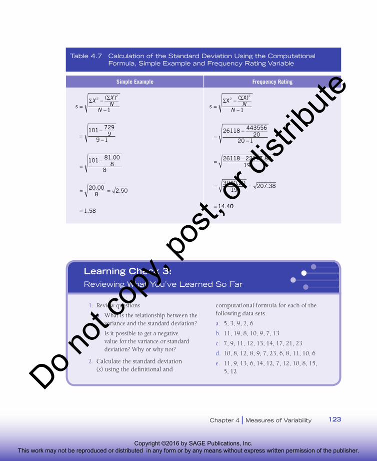
Computational Formula for the Standard DeviationThe computational formula for the standard deviation (Formula 4-6) simply places the computa-tional formula for the variance (Formula 4-4) within the square root symbol:

s NN

=−

−

Σ ΣX X22

1

( ) (4-6)

The standard deviation for the simple example of nine scores and the frequency rating variable are calculated using Formula 4-6 in Table 4.7 (the values for the sum of scores squared [(ΣX)2] and the sum of squared scores [ΣX2] for the two examples are found in Tables 4.5 and 4.6). Similar to the variance, note the same value for the standard deviation is obtained regardless of whether the definitional or computational formula is used.


Do not

copy

, pos

t, or d

istrib

ute


Table 4.7 Calculation of the Standard Deviation Using the Computational Formula, Simple Example and Frequency Rating Variable

Simple Example Frequency Rating

s NN

=−

−

Σ ΣX X22

1

( )

=−

−

=−

= =

=

101 7299

9 1

101 81 008

8

20 008

2 50

1 58

.

. .

.

s NN

=−

−

Σ ΣX X22

1

( )

=−

−

= −

= =

=

26118 44355620

20 1

26118 22177 8019

3940 2019

207 38

14 4

.

. .

. 00

1. Review questions

a. What is the relationship between the variance and the standard deviation?

b. Is it possible to get a negative value for the variance or standard deviation? Why or why not?

2. Calculate the standard deviation (s) using the definitional and

computational formula for each of the following data sets.

a. 5, 3, 9, 2, 6

b. 11, 19, 8, 10, 9, 7, 13

c. 7, 9, 11, 12, 13, 14, 17, 21, 23

d. 10, 8, 12, 8, 9, 7, 23, 6, 8, 11, 10, 6

e. 11, 9, 13, 6, 14, 12, 7, 12, 10, 8, 15, 5, 12



Do not

copy

, pos

t, or d

istrib

ute


4.7 Measures of Variability for Populations

The formulas for the variance and standard deviation described thus far are used for samples drawn from populations. But what if you were to collect data from the entire population? This section discusses two measures of variability for populations: the population variance and the population standard deviation.

The Population Variance (σ2)The variance for data collected from a population is called the population variance (σ2) (σ is the lowercase Greek letter sigma), which is defined as the average squared deviation of a score from the population mean. The definitional formula for the population variance is provided in Formula 4-7:

σ22

= −Σ( )X µN

(4-7)

where X is a score for a variable, µ is the population mean, and N is the total number of scores.The formula for the population variance differs from the formula for the variance s2 (Formula

4-4) in two important ways. First, the mean in the formula is the population mean µ rather than the sample mean X . Second, the sum of the squared deviations (Σ(X – μ)2) is divided by N rather than N – 1; this is because you are no longer estimating the variability in the population from data collected from a sample but instead have collected data from the entire population.

Imagine, for a moment, that the nine scores in the first column of Table 4.3 represent a pop-ulation rather than a sample. Using the squared deviations for these scores calculated in the last column of Table 4.3, the population variance would be equal to the following:

σ2

2

= −Σ( )X µN

= 1 00 00 4 00 1 00 9 00 009

20 009

. . . ... . . . .+ + + + + + =

= 2.22

From this calculation, you would conclude that, assuming these nine scores represent the entire population, the average squared deviation of a score from the population mean of 3.00 is 2.22.

The Population Standard Deviation (σ)Calculating the population variance involves squaring the deviation of each score from the popula-tion mean µ. In order to obtain a measure of variability that represents the average deviation (rather than the average squared deviation) from the population mean, the square root of the population variance may be calculated. This is the population standard deviation (σ), defined as the square


Do not

copy

, pos

t, or d

istrib

ute


root of the population variance. Mathematically, the population standard deviation is the square root of the average squared deviation from the population mean, and it represents the average deviation of a score from the population mean. Formula 4-8 provides the definitional formula for the popula-tion standard deviation.

σ = −Σ( )X µ 2

N (4-8)

Relying again on Table 4.3, the population standard deviation for the set of nine scores is cal-culated below.

σ = −Σ( )X µ 2

N

= 1 00 00 4 00 1 00 9 00 00

9. . . ... . . .+ + + + + +

= 209

2 22= .

= 1.49

From these calculations, it may be concluded that the average deviation of the nine scores from the population mean of 3.00 is equal to 1.49.

Measures of Variability for Samples vs. PopulationsThe population variance and standard deviation are examples of parameters, which were intro-duced in Chapter 3. Parameters are numeric characteristics of populations and are distinguished from statistics, which are numeric characteristics of samples. Parameters are calculated when data are collected from the entire population, whereas statistics are calculated when data are collected from a sample drawn from a larger population. This is summarized below for both a measure of central tendency (the mean) and a measure of variability (the standard deviation):

Target Numeric Characteristic Mean Standard Deviation

Sample statistic X s

Population parameter μ σ

Because researchers rarely collect data from entire populations, statistics such as the sample mean and standard deviation are much more likely to be calculated than population parameters. Throughout this book, when you see the words mean, variance, or standard deviation, you should assume they refer to samples rather than populations. In fact, numeric values of parameters such as μ or σ are typically values believed or hypothesized to be true rather than values based on the actual collection of data.


Do not

copy

, pos

t, or d

istrib

ute


4.8 Measures of Variability: Drawing Conclusions

These early chapters of this book have discussed the importance of examining and drawing appropri-ate conclusions about three aspects of distributions: modality, symmetry, and variability. Measures of central tendency such as the mean, median, and mode provide a numerical description of the modality and, to a lesser degree, the symmetry of a variable by focusing on the center of the distribution and what scores have in common with each other. However, it is equally important to consider the variabil-ity in a distribution, which is the degree to which scores differ from the center of the distribution and from each other. Measures of variability such as the variance and standard deviation provide valuable information, for example, regarding the degree to which participants in a sample agree when asked the same survey question or respond in a similar manner to the same experimental manipulation.

The beginning of this chapter introduced a research study designed to measure the degree to which people differ in their interpretation of words such as sometimes, often, and seldom. Based on the variability of the frequency ratings, what did these researchers conclude regarding the degree to which people agree in their perceptions of these words? Comparing the results of their study with those conducted in other countries, they concluded the following:

There are subtle variations in how those sharing the same language describe the interme-diate points . . . so it cannot be assumed that rating scales developed in one culture can be automatically used in another, even where there is a common language. (Skevington & Tucker, 1999, p. 59)

4.9 Looking Ahead

Several critical issues have been identified and discussed in the first four chapters of the book. The first is the importance of examining data before conducting statistical analyses on the data.

1. Review questions

a. What is the main difference between the population standard deviation and the standard deviation?

b. Under what conditions would you calculate the population standard deviation for a set of data rather than the standard deviation?

2. Calculate the population standard

deviation (σ) using the definitional and computational formula for each of the following data sets:

a. 2, 4, 5, 6, 8

b. 8, 6, 4, 8, 3, 7

c. 71, 84, 65, 78, 89, 72, 60, 85

d. 3.0, 1.5, 3.5, 3.0, 2.0, 2.5, 4.0, 1.0, 2.0

e. 10, 8, 12, 8, 9, 7, 23, 6, 8, 11, 10, 6



Do not

copy

, pos

t, or d

istrib

ute

Appropriate and meaningful conclusions cannot be drawn from statistical analyses until the accu-racy of the data has been confirmed and the distribution of scores has been understood. Second, there are many different types of distributions; you have seen distributions labeled as symmetric, skewed, peaked, flat, unimodal, and bimodal. Third, distributions can be described numerically using measures of central tendency and variability. The next chapter discusses yet another type of distribution: “normal distributions.” Like the other distributions discussed so far, normal distribu-tions can be described using descriptive statistics such as measures of central tendency and vari-ability. What makes normal distributions unique, as we will discuss in greater detail going forward, is that they possess characteristics that enable them to be the basis of a second type of statistics, known as “inferential statistics,” whose goal is to test hypotheses about populations based on the information from samples.

4.10 SUMMARY

Variability is a third aspect of distributions and refers to the amount of spread or scat-ter of scores in a distribution. One goal of a science such as psychology is to describe, understand, explain, and predict variability in the phenomena studied by researchers.

A measure of variability is a descriptive statistic of the amount of differences in a set of data for a variable. Common measures of vari-ability are the range, the interquartile range, the variance, and the standard deviation.

The range is the mathematical differ-ence between the lowest and highest scores in a set of data. The interquartile range is the range of the middle 50% of the scores for a variable, calculated by removing the highest and lowest 25% of the distribution. The variance (s2) is the average squared deviation of a score from the mean. The standard deviation (s) is the square root of the variance, and it represents the average deviation of a score from the mean. Because the variance and standard deviation (unlike the range and interquartile range) are based on all of the scores in the distribution, they can be used in statistical analyses designed to test hypotheses about distributions.

The variance and the standard devia-tion may be calculated either using a defi-nitional formula, which is a formula based on the actual or literal definition of a con-cept, or a computational formula, defined as a formula not based on the definition of a concept but is designed to simplify mathe-matical calculations. Computational formu-las are used because using the definitional formula in a large or complicated data set increases the chances of making computa-tional errors.

The variance and standard deviation measure the variability in data collected from samples drawn from populations; the population variance (σ2) (the average squared deviation of scores from the pop-ulation mean) and the population standard deviation (σ) (the square root of the pop-ulation variance) are calculated when data are collected from the entire population. Because data are rarely collected from entire populations, numeric values of parameters such as σ are typically based on beliefs and hypotheses rather than the actual collection of data.



Do not

copy

, pos

t, or d

istrib

ute


4.11 IMPORTANT TERMS

measure of variability (p. 107)

range (p. 108)

interquartile range (p. 110)

variance (s2) (p. 114)

definitional formula (p. 116)

computational formula (p. 116)

biased estimate (p. 120)

unbiased estimate (p. 120)

standard deviation (s) (p. 120)

population variance (σ2) (p. 124)

population standard deviation (σ) (p. 124)

4.12 FORMULAS INTRODUCED IN THIS CHAPTER

Range

Range = highest score – lowest score (4-1)

Interquartile Range


)th score – ( N4

+ 1)th score (4–2)

Variance (s2) (Definitional Formula)

s22

1= −

−Σ( )X X

N (4-3)

Variance (s2) (Computational Formula)

s N

N2

22

1=

−

−

Σ ΣX X( ) (4-4)

Standard Deviation (s) (Definitional Formula)

s XN

= −−

Σ( )X 2

1 (4-5)

Standard Deviation (s) (Computational Formula)

s N

N=

−

−

Σ ΣX X22

1

( ) (4-6)


Do not

copy

, pos

t, or d

istrib

ute

Population Variance (σ2) (Definitional Formula)

σ22

= −Σ( )X µN

(4-7)

Population Standard Deviation (σ) (Definitional Formula)

σ = −Σ( )X µ 2

N (4-8)

4.13 USING SPSS

Calculating Measures of Central Tendency and Variability: The Frequency Rating Study (4.1)

1. Define variable (name, # decimal places, label for the variable) and enter data for the variable.

2. Select the descriptive statistics procedure within SPSS.How? (1) Click Analyze menu, (2) click Descriptive Statistics, and (3) click Descriptives.



Do not

copy

, pos

t, or d

istrib

ute


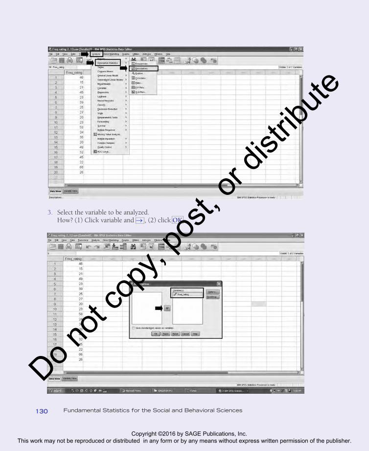
3. Select the variable to be analyzed.How? (1) Click variable and → , (2) click OK .


Do not

copy

, pos

t, or d

istrib

ute

4. Examine output.

4.14 EXERCISES


a. 4, 6, 9

b. 14, 17, 11, 19, 12

c. 25, 22, 27, 30, 21, 26, 29

d. 10, 8, 4, 16, 9, 7, 9, 13, 6, 11

e. 73, 66, 91, 84, 69, 87, 62, 79, 82, 90

f. 3.50, 4.21, 3.95, 2.27, 3.06, 4.58, 2.74, 3.89, 2.65, 2.03, 4.41, 3.76, 2.35


a. 9, 10, 13

b. 5, 3, 9, 12

c. 6, 2, 8, 12, 9, 5, 7

d. 8, 4, 1, 6, 14, 9, 12, 5, 11, 7, 4

e. 16.65, 12.98, 31.74, 18.80, 27.31, 29.92, 34.65, 23.68, 28.20, 20.77


a. 3, 6, 7, 12, 15, 17, 23, 28

b. 8, 4, 1, 6, 13, 10, 12, 5

c. 3, 8, 14, 11, 16, 7, 14, 15, 11, 9, 12, 6

d. 15, 22, 17, 13, 31, 25, 22, 19, 26, 30, 27, 19, 23, 21, 27, 29

e. 450, 560, 340, 510, 390, 670, 540, 420, 720, 480, 560, 510

f. 29, 27, 26, 15, 28, 26, 32, 27, 26, 25, 30, 26, 27, 18, 23, 35


a. 1, 2, 2, 3, 4, 5, 7, 10

b. 21, 8, 17, 7, 12, 19, 5, 12

c. 6, 9, 5, 14, 3, 15, 19, 7, 13, 6, 8, 5

d. 6.78, 7.81, 6.35, 9.65, 5.43, 8.62, 5.90, 7.13, 6.56, 3.27, 8.92, 4.49

e. 78, 55, 82, 64, 93, 69, 71, 82, 59, 71, 76, 52, 89, 75, 81, 78

5. For each of the following sets of data, (1) calculate the mean of the scores ( X ), (2) calculate the deviation of each score from the mean (X – X ), and (3) check to see if the sum of the deviations equals zero (Σ(X – X ) = 0).

Descriptive Statistics

N Minimum Maximum Mean Std. Deviation

Freq_ratingValid N (listwise)

2020

15 66 33.30 14.401

StandarddeviationN Mean



Do not

copy

, pos

t, or d

istrib

ute


a. 2, 4, 6

b. 5, 6, 13

c. 4, 7, 8, 9

d. 5, 2, 7, 13, 11

e. 3, 8, 14, 11, 16, 7, 14, 15, 11

6. For each of the following sets of data, (1) calculate the mean of the scores ( X ), (2) calculate the deviation of each score from the mean (X – X ), and (3) check to see if the sum of the deviations equals zero (Σ(X – X ) = 0).

a. 7, 5, 12

b. 6, 7, 9, 12

c. 6, 8, 4, 11, 3, 7

d. 5, 7, 3, 1, 4, 8, 5, 2, 7, 9, 12, 4, 15

7. For each of the sets of data in Exercise 5, calculate the variance (s2) using the definitional formula and the computational formula.

8. For each of the sets of data in Exercise 5, calculate the population variance (σ2) using the definitional formula. Comparing your calculations for each data set with those done in Exercise 7, which is larger, the variance or the population variance? Why?

9. For each of the sets of data in Exercise 5, calculate the standard deviation (s) and the population standard deviation (σ). For each data set, which is larger, the standard deviation or the population standard deviation?

10. (This example was discussed in Chapters 2 and 3.) A friend of yours asks 20 people to rate a movie using a 1- to 5-star rating: the higher the number of stars, the higher the recommendation. Their ratings are listed below:

a. Calculate the variance (s2) and standard deviation (s) of the ratings using either the definitional or the computational formulas. (Note: From Chapter 3, you may have already calculated the number of scores (N), sum of scores squared ((ΣX)2), the sum of squared scores (ΣX2), and the mean ( X ).)

Person # Stars Person # Stars

1 11

2 12

3 13

4 14

5 15

6 16

7 17

8 18

9 19

10 20


Do not

copy

, pos

t, or d

istrib

ute

b. Based on your value of the standard deviation, what would you conclude regarding the degree to which these people agree or disagree about this movie?

11. One study stated the research hypothesis, “Violence behavior in children may be reduced by teaching them conflict resolution skills” (DuRant et al., 1996). The variable “violence behavior” was measured by the number of fights in which each student was involved. Below is a frequency distribution table for the number of fights for 12 students.

# Fights f % # Fights f %

4 1 8% 1 1 8%

3 2 17% 0 3 25%

2 5 42% Total 12 100%

a. Calculate the variance (s2) and standard deviation (s) of the number of fights using either the definitional or the computational formulas.

b. Based on your value of the standard deviation, what is the average difference between the number of fights a student got involved in and the mean?

12. (This example was introduced in Chapter 3). The 10% myth study discussed in this chapter measured the beliefs of both psychology majors and non–psychology majors. The 39 non–psychology majors in this study provided the following values for the brain power variable:

Non–Psychology

MajorEstimated

Brain Power

Non–Psychology

MajorEstimated

Brain Power

Non–Psychology

MajorEstimated

Brain Power

1 15 14 10 27 15

2 45 15 20 28 25

3 10 16 50 29 10

4 40 17 25 30 20

5 5 18 45 31 10

6 10 19 40 32 5

7 50 20 25 33 15

8 45 21 10 34 10

9 10 22 5 35 5

10 10 23 15 36 60

11 35 24 5 37 10

12 5 25 40 38 5

13 15 26 30 39 15



Do not

copy

, pos

t, or d

istrib

ute


a. Calculate the variance (s2) and standard deviation (s) of the estimates using either the definitional or the computational formulas. (Note: From Chapter 3, you may have already calculated the number of scores (N), sum of scores squared ((ΣX)2), the sum of squared scores (ΣX2), and the mean ( X ).)

13. (This example was introduced in Chapter 2.) An instructor administers a 27-item quiz to her class of 25 students. Each student’s score on the quiz is the number of items answered correctly. These scores are listed below:

Person Quiz Score Person Quiz Score Person Quiz Score

1 22 10 17 19 20

2 15 11 18 20 21

3 11 12 14 21 17

4 19 13 10 22 18

5 12 14 6 23 15

6 21 15 16 24 24

7 22 16 20 25 22

8 19 17 21

9 23 18 19

a. Calculate the variance and standard deviation of the ratings using the computational formulas.

14. On your own, create two distributions of 10 scores that have the same mean but differ in modality: one unimodal and one bimodal. Calculate the standard deviation off the two distributions. Is there greater variability in the unimodal distribution or the bimodal distribution?

15. On your own, (a) create two distributions of 10 scores that have the same mean but differ in their amount of variability, and (b) create two distributions of 10 scores that have different means but have the same amount of variability. (c) What does this imply about the information that is necessary to accurately describe a distribution of scores for a variable?

16. What if someone told you, “There is very little variability in the scores for my variable.” From this statement, would you be more likely to describe the shape of the distribution as peaked or flat?

17. What if someone told you, “There is a great deal of variability in the scores for my variable.” From this statement, can you tell whether the shape of the distribution is symmetrical or skewed? Why or why not? If not, what would you do to determine the symmetry of the distribution?

18. What if someone told you, “The mean age of the participants in this sample was 35.50 and the standard deviation was 2.53.” Why would you interpret the sample differently if you had been told the standard deviation was 14.71?


Do not

copy

, pos

t, or d

istrib

ute

19. An employment survey in 2009 was conducted to find the average starting salaries of people receiving doctorate (PhD) degrees in psychology (Michalski, Kohout, Wicherski, & Hart, 2011). The mean starting salary for psychologists in assistant professor positions in universities was approximately $60,000 with a standard deviation of $11,000. Clinical psychologists in their first year of practice also report a mean of approximately $60,000 but with a standard deviation of $16,000.

a. Which type of psychologist has more variability in income?

b. For which type of psychologist could you more accurately predict a salary for, and why?

Answers to Learning Checks

Learning Check 1

2. a. Range = 6

b. Range = 12

c. Range = 19

d. Range = .90

3. a. Interquartile range = 3

b. Interquartile range = 8

c. Interquartile range = 1

d. Interquartile range = .30

Learning Check 2

2. a. s2 = 4.00

b. s2 = 4.00

c. s2 = 17.07

d. s2 = 105.79

e. s2 = 1.84

Learning Check 3

2. a. s = 2.74

b. s = 4.04

c. s = 5.33

d. s = 4.55

e. s = 3.12



Do not

copy

, pos

t, or d

istrib

ute


Learning Check 4

2. a. σ = 2.00

b. σ = 1.91

c. σ = 9.58

d. σ = .91

e. σ = 4.36

Answers to Odd-Numbered Exercises

1. a. Range = 5

b. Range = 8

c. Range = 9

d. Range = 12

e. Range = 29

f. Range = 2.55

3. a. Interquartile range = 10

b. Interquartile range = 5

c. Interquartile range = 6

d. Interquartile range = 8

e. Interquartile range = 110

f. Interquartile range = 2

5. a. Score (X) Mean ( X ) Mean (X – X )

2 4.00 –2.00

4 4.00 .00

6 4.00 2.00

Σ(X – X ) = 0

b. Score (X) Mean ( X ) Mean (X – X )

5 8.00 –3.00

6 8.00 –2.00

13 8.00 5.00

Σ(X – X ) = 0


Do not

copy

, pos

t, or d

istrib

ute

Score (X) Mean ( X ) Score – Mean (X – X )

4 7.00 –3.00

7 7.00 .00

8 7.00 1.00

9 7.00 2.00

Σ(X – X ) = 0

c.

d. Score (X) Mean ( X ) Score – Mean (X – X )

5 7.60 –2.60

2 7.60 –5.60

7 7.60 –.60

13 7.60 5.40

11 7.60 3.40

Σ(X – X ) = 0

e. Score (X) Mean ( X ) Score – Mean (X – X )

3 11.00 –8.00

8 11.00 –3.00

14 11.00 3.00

11 11.00 .00

16 11.00 5.00

7 11.00 –4.00

14 11.00 3.00

15 11.00 4.00

11 11.00 .00

Σ(X – X ) = 0

7. a. s2 = 4.00

b. s2 = 19.00

c. s2 = 4.67

d. s2 = 19.80

e. s2 = 18.50



Do not

copy

, pos

t, or d

istrib

ute


9. a. s = 2.00, σ = 1.63

b. s = 4.36, σ = 3.56

c. s = 2.16, σ = 1.87

d. s = 4.45, σ = 3.98

e. s = 4.30, σ = 4.06

Note: In all data sets, the standard deviation (s) is larger than the population standard deviation (σ) because you are dividing by a smaller number (N – 1 rather than N).

11. a. s2 = 1.66, s = 1.29

b. The average difference between the number of fights of a student and the mean is 1.29 fights.

13. a. s2 = 19.89, s = 4.46

15. a. Sample Data Set 1: 4, 4, 5, 5, 5, 5, 5, 6, 6, 6 X = 5.10, s = .74

Sample Data Set 1: 2, 2, 3, 4, 5, 5, 6, 6, 9, 9 X = 5.10, s = 2.51

b. Sample Data Set 3: 3, 3, 4, 4, 5, 5, 5, 6, 7, 7 X = 4.90, s = 1.45

Sample Data Set 4: 8, 8, 9, 9, 10, 10, 10, 11, 12, 12 X = 9.90, s = 1.45

c. Distributions with the same mean or the same standard deviation can be describing very different information; therefore, it is important to provide both measures of central tendency and variability to describe a set of data.

17. There can be a great deal of variability in both symmetrical and skewed distributions. The simplest way to determine the symmetry of a distribution is to look at a figure of the distribution.

19. a. Clinical psychologists have more variability in their starting salaries.

b. You could more accurately predict the income for a psychologist going into an assistant professor position because there is less variability in their starting salaries.

Sharpen your skills with SAGE edge at edge.sagepub.com/tokunaga

SAGE edge for students provides a personalized approach to help you accomplish your coursework goals in an easy-to-use learning environment. Log on to access:

• eFlashcards• Web Quizzes• Chapter Outlines

• Learning Objectives• Media Links• SPSS Data Files


Do not

copy

, pos

t, or d

istrib

ute

chapter 4 measures of variability distribute · introduces measures of variability, which are...

Documents