chapter 4: individual and market demand - university …web.uvic.ca/~okhan/ch 4 individual and...

Econ 203 Chapter 4 page 1

Chapter 4: Individual and Market Demand Overview: Chapter 4 + 5.1-5.3: Implications of optimal choice What happens if income changes? What happens to individual demand if a price changes? ►Individual demand function ►From individual demand to market demand ►Market demand and changes in prices or income ►The impact importance of a market for consumers ►Consumer surplus: Willingness to pay versus actual pay


The Environment: competitive markets Price taking assumption: There is one (per-unit) price that everybody takes as given. ▪Impersonal market ▪No haggling, bluffing, or other forms of strategic behaviour to influence prices.


The Price Elasticity of Demand and Supply

Price Elasticity is a unitless measurement of the sensitivity of the quantity demanded or supplied to a change in the price.

This sensitivity measures how much the firm’s total revenue will change in response to a price change.

Total revenue increases or decreases depending on how large the percentage change in the quantity demanded is relative to the percentage change in the price. Hence, the price elasticity of demand determines whether revenue will rise or fall.


Price Elasticity of Demand “The price elasticity of demand measures the percentage change in the quantity demanded relative to the percentage change in price.” If the percentage change in the quantity demanded is larger than the percentage change in price, total revenue will change in the opposite direction to the price change. Let R=PQ (Total Revenue) i.e. P increases →Q decreases→If Q is > P→TR decreases The change in TR is negative.


Price P1 A B P2 0 Q1 Q2 Quantity At price P1, the quantity demanded is Q1. Total revenue= P1*Q1. Suppose price falls: At the new lower price of P2, the quantity demanded is Q2. → Total revenue is P2*Q2.

Demand

At the lower price, the firm can sell more units and TR increases.

In this case, total revenue increases, but this is not always the case.


It depends on how sensitive a change in quantity demanded is to a change in price. The response of revenue to a change in price will result in demand being: (1) price elastic if total revenue increases (decreases) when the change in price decreases (increases). (2) unitary elastic if total revenue does not change when the price changes. (3) price inelastic if the total revenue changes in the same direction that the price changes.


(I) Point Price Elasticity of Demand (small price changes) The point price elasticity of demand measures the sensitivity of the quantity demanded to a change in price starting at a point on the demand curve. The sign of this elasticity is negative. Hence, it is customary to report the absolute value of the elasticity of demand. If something is price elasticity| ηp | >1. If something is price inelastic, | ηp |<1.


η

η ∂∂

P

P

QQPP

QP

PQ

QP

PQ

= = • ⇐

= ×

Δ

ΔΔΔ

Point Elasticity of Demand

*Note: With straight-line demand functions, the numerical value of the price elasticity is different at different points along the demand function because Δ ΔQ P and/or P/Q will change. Only in some ‘special’ cases this does not hold.


Figure 1: Demand Curve With Zero Price Elasticity of Demand

Price Demand Curve

0 Quantity

Demand curve has a price elasticity of zero: ηp =0. Quantity demanded is unaffected by price. Example: Insulin


Figure 2: Demand Curve with Infinite Price Elasticity of Demand

Price Demand Curve 0 Quantity

Demand curve price elasticity equals infinity: ηp =∞ . →Unlimited amount can be sold at a particular price. Example: interest rates on GICs.

Nothing can be sold if the price if the price is increased slightly.


Figure 3: Values of the Price Elasticities Of Demand Along a Linear Demand Curve

Price ηp =∞ ηp is elastic Unitary Elasticity ηp is inelastic Demand 0 MR ηp $, TR Max TR

00 Q* Quantity

If demand is price elastic, MR is positive and as Quantity increases, TR increases

Demand curve: P=a-bQ


(II) Arc Price Elasticity of Demand (large price changes) Also measures the percentage change in quantity relative to the percentage change in price. Arc Price Elasticity: equals the change in quantity relative to the average quantity demanded divided by the change in price relative to the average price.

ηp

QQ Q

PP P

QP

P PQ Q

=+

+

= •++

Δ

ΔΔΔ

( )

( )

1 2

1 2

1 2

1 2

2

2


Things to Note: The arc elasticity is:

(i) always negative because Δ ΔQ P is negative. I.e. the price and quantity demanded will change in the opposite direction.

(ii) not equal to the slope of the demand function.

The value of the arc price elasticity dictates whether revenue increases, decreases or remains the same when price changes.


Just like the point elasticity of demand, the arc elasticity of demand has three possible outcomes:

1) If arc price elasticity is less than -1, demand is considered price elastic.

Total revenue will change in the opposite direction to the price change. An increase in price leads to a decrease in total revenue.


2) If arc price elasticity is equal to -1, demand has unitary elasticity.

A change in price does not change total revenue.

3) If arc price elasticity is between -1 and 0, demand is price- inelastic.

Total revenue will change in the same direction as the price change. An increase in price leads to an increase in revenue.


Factors That Determine the Size of Price Elasticity of Demand 1. The higher the percentage of a consumer’s total income spent

on a good, the more price-elastic is the demand for that good. Expensive items are very price sensitive. Small changes in price, may lead to large changes in quantity demanded. 2. The more substitute products, the more demand will be price-

elastic. If the price of one type of cel-phone increases by a small amount, the demand for that phone may dramatically drop. This is because there are many substitute phones that offer the same quality of service.


3. As income rises and consumers continue to spend an increasing proportion of their increasing income on a good, these goods also have more elastic demand functions, other things remaining the same.

Examples: Houses, cars, vacations, etc.. 4. Time: the more time for consumers to gather information about

substitute products, the more price elastic is the demand for the good. In the short-run, a price change may have very little affect on the quantity of the good demanded. But, in the long-run, as consumers become more informed about substitute products, this price change may have a more dramatic affect on the quantity demanded. Hence, price increases may be a big mistake in the long-run.


Price C B P2 P1 A DL Long-Run Demand DS Initial Demand 0 Q3 Q2Q1 Quantity As time goes by, consumers become more aware of alternative products. The demand function becomes more elastic in the long-run.


The Market Demand Function To derive the market demand function, we will use the utility maximization model of consumer behaviour to determine each consumer’s demand function for a good. The Consumer’s Demand Function Assume: the consumer’s income is fixed two goods, X and Y price of Y is fixed


Y1 A C Y3 B Y2 I3 I1 Qx Price of X P1 P2 P3 dx= individual demand 0 X1 X2 X3 Qx

I2

Qy

As the price of X decreases, the budget constraint rotates.

The consumer purchases different baskets to maximize utility.

The demand curve for good X is derived as the price of X changes.


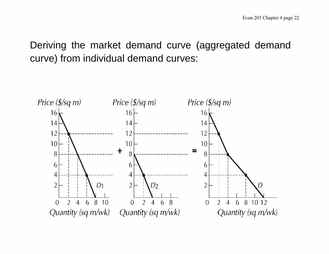
The Market Demand Function The market demand function represents the total quantity of a good demanded by all individuals at each price. It is derived by summing up horizontally the demand curve of each consumer. For each price, the quantity demanded by each consumer is added up horizontally to derive the total quantity demanded in the market. Individual demand curves differ because income and preferences differ across consumers.


Deriving the market demand curve (aggregated demandcurve) from individual demand curves:


Substitutes and Complements When the price of a good changes and the quantity demanded of another good changes in the opposite direction, with the price of the other good held constant, the two goods are referred as complement goods. QB PA D0 D1 B Px I 1 A I0 0 X1 X2 QA X1 X2 QA

Demand for good A increases due to a decrease in the price of B.


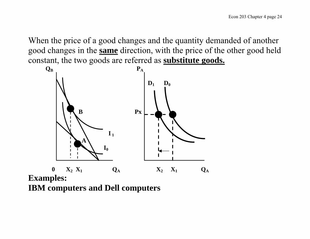
When the price of a good changes and the quantity demanded of another good changes in the same direction, with the price of the other good held constant, the two goods are referred as substitute goods. QB PA D1 D0 B Px I 1 A I0 0 X2 X1 QA X2 X1 QA Examples: IBM computers and Dell computers


We can determine whether two goods are substitutes or complements by the sign of the arc cross-price elasticity of demand. The arc cross-price elasticity of demand measures the average percentage change in the quantity of one good relative to the average percentage change in the price of another. If we have two goods A and B, the arc cross-price elasticity of demand is:

EBP

P PB BBP

A

A AA= •

++

ΔΔ

1 2

1 2


The only difference with this equation with the arc price elasticity of demand is that the change in the quantity of A has been replaced by the change in the quantity of B, and the sum of the units of A by the sum of the units of B. The arc cross-price elasticity of demand measures the response of B to a change in the price of A.

If A and B are complements, then ΔΔ

BPA

is negative and the arc cross price elasticity of demand is negative.

If A and B are substitutes, then ΔΔ

BPA

is positive and the arc cross price elasticity of demand is positive.


Extending the Theory of Consumer

Behaviour 1) The Shape of the Consumer’s Demand Function Income Effect Substitution Effect Slope of the Demand Function 2) Consumer Surplus Marginal Value


The Shape of the Consumer’s Demand Function Recall, consumers have different individual demand functions and indifference curves for goods. If the price of a good is increased, some consumers will reduce their consumption of the good by a large amount, while other consumers will reduce their consumption by a modest amount. This is because consumers have different preferences and income levels.


In order to examine the factors that explain the different responses these differences create, we will decompose the effects into what is referred to as the income effect and the substitution effect. ►Suppose the price a good ‘X’ decreases. How does the consumer respond? A price decrease in X can be viewed as a release in income formerly used to purchase units of X. These ‘$’s’ represent an increase in disposable income that can be used to purchase more of good X or more of other goods.


This increase in disposable income can be graphically illustrated as a shift outward of the budget constraint. As a result of the shifting budget constraint, the consumer can select a new market basket on a higher indifference curve. So: “The change in quantity demanded of good X due to the change in money

income is the income effect.


But, a price cut also has a substitution effect that must be considered. With a price cut, good X is now cheaper relative to other goods than before. The consumer will now demand more units of the cheaper good and fewer units of other goods while remaining at the same level of satisfaction (same indifference curve).


The substitution effect measures the change in the quantity demanded due to a change in the relative price of X

holding utility constant. ►Hence, we assume the consumer separates the total change in the quantity demanded of X caused by a price change into these two effects.


The Income Effect: Normal Good Other B S1 A S0 X0 X1 Units of X If the consumer’s income increases to BL1, there will be a parallel shift outward by budget line.

BL0 I0

I1

BL1

I-C Curve


The consumer can now purchase market bundle B on the higher indifference curve I1, which is tangent to the higher budget constraint.

In this case, more of both goods are purchased When the quantity demanded of a good changes in the same direction as the change in income, the good is referred to as a normal good. Note: For every level of income there is point of

tangency between the budget constraint and an indifference curve. By connecting these points, we form what is known as the income-consumption curve.


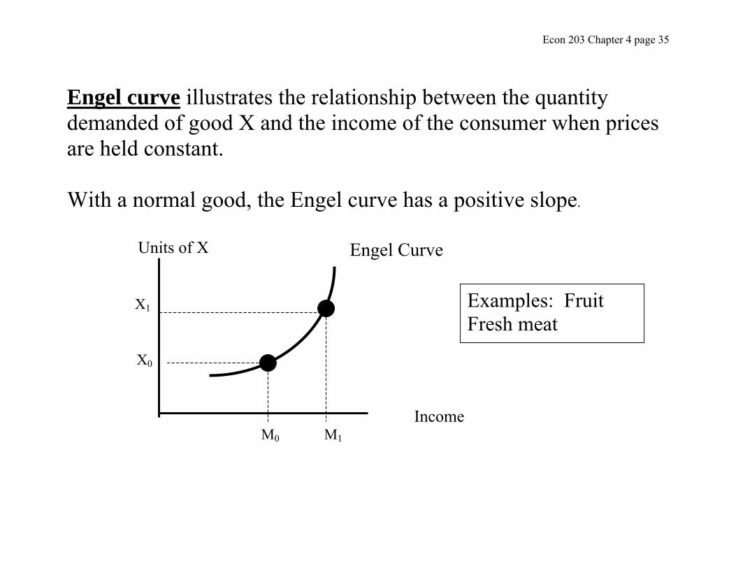
Engel curve illustrates the relationship between the quantity demanded of good X and the income of the consumer when prices are held constant. With a normal good, the Engel curve has a positive slope. Units of X X1 X0 Income M0 M1

Engel Curve

Examples: Fruit Fresh meat


The Income Effect: Inferior Good Other S1 B S0 A X1 X0 Units of X The diagram illustrates how a consumer’s consumption choice changes when income has increased.

BL0

I0

I1

BL1

I-C Curve


If the consumer’s income increases to BL1, there will be a parallel shift outward by the budget line. The consumer can now purchase market bundle B on the higher indifference curve I1, which is tangent to the higher budget constraint. In this case, less of good X and more of other goods are purchased. When the quantity demanded of a good changes in the opposite direction as the change in income, the good is referred to as an inferior good.


With an inferior good, the Engel curve has a negative slope. Units of X X0 X1 Income M0 M1

This is because the quantity demanded decreases when income increases holding prices constant. Note: Inferior goods are not inferior to all consumers at all income levels.

Engel Curve

Examples: Hamburger used cars used shoes


Income Elasticity of Demand Income elasticity of demand measures the response of a percentage change in the quantity demanded due to a percentage change in income. The point income elasticity of demand:

ηM

x

X x

X

QQ

IncomeM

QM

MQ

= = •

Δ

ΔΔΔ


The point measure of income elasticity is the percentage change in quantity

demanded divided by the percentage change in income.

The arc income elasticity of demand:

( )

( )

( )( )ηM

x

X X x

X X

QQ Q

IncomeM M

QM

M MQ Q

=+

+

= •++

Δ

ΔΔΔ

0 1

0 1

0 1

0 1

2

2


ηM is positive for a normal good (I.e. the quantity demanded increases when income increases,) and is negative for an inferior good. (I.e. quantity demanded decreases when income increases. Of course, even if a good is classified to be normal, this does not guarantee that a consumer will continue to spend an increasing proportion of income on it as his or her income increases. This will only occur if the income elasticity of demand is greater than 1. ηM >1

Examples: Vacations


If the income elasticity of demand is between zero and 1, a good is a normal good but the consumer spends a decreasing proportion of income on it as income rises, assuming that price has remained the same. 0 < ηM <1 Examples: food Clothing Soap


Substitution Effect: Other Goods S0 A S1 B 0 X0 X1 Units of X

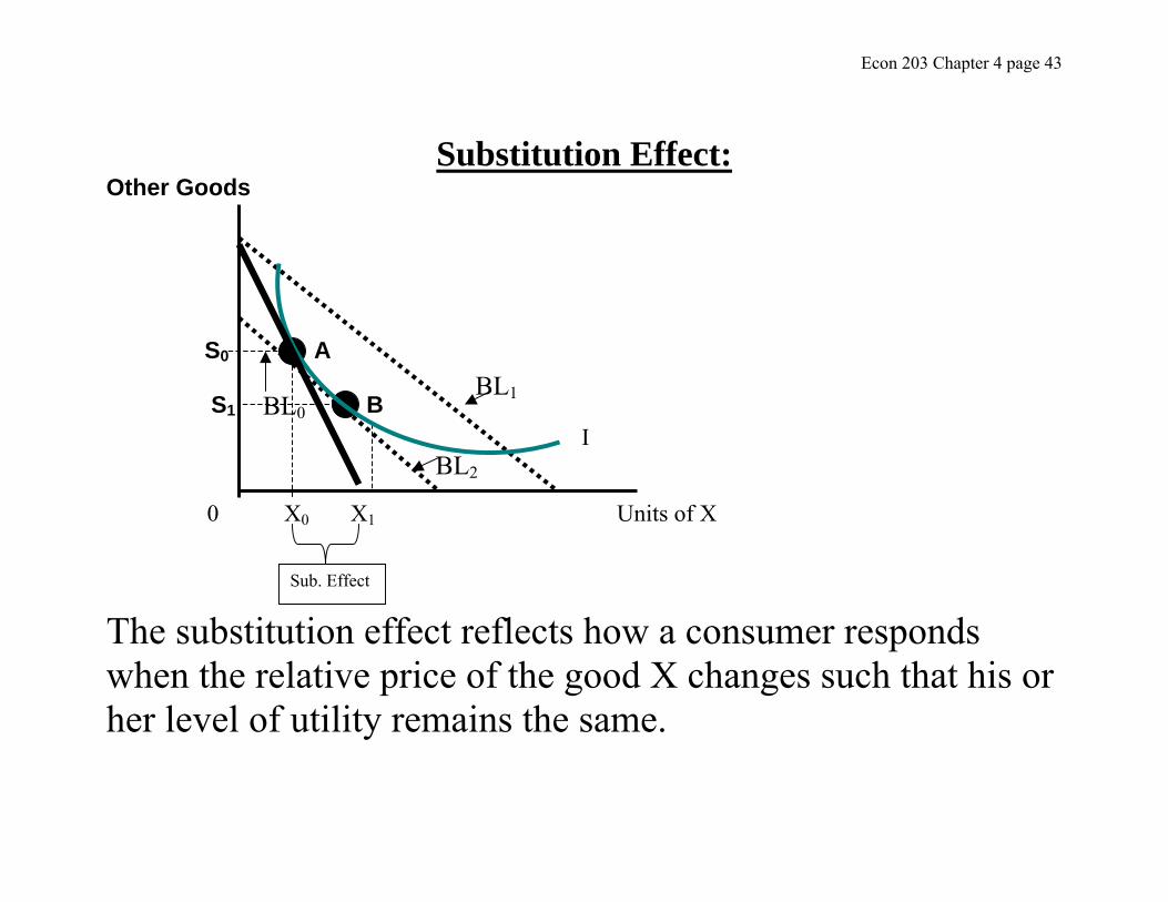
The substitution effect reflects how a consumer responds when the relative price of the good X changes such that his or her level of utility remains the same.

BL2

BL0 I

BL1

Sub. Effect


If the price of the good X falls, the budget constraint rotates outward. We know that the consumer will purchase a different market basket of goods on a higher indifference curve. Hence the utility of the consumer will increase. But, the substitution effect measures the change in the quantity demanded when the relative prices change with utility held constant.


In order to keep the consumer on the original indifference curve and maintain the original level of utility, we change money income as the price changes by just enough so that the consumer finds a new market basket on the original indifference curve where the slope of the new budget constraint equals the slope of the indifference curve. The quantity of X demanded increases to X1. Since the relative price of X is lower, budget line BL2 is flatter than BL0.


The consumer’s response to a relative price decrease in X is to purchase more units of good X and spend less on other goods. The sign of the substitution effect is negative because a change in the relative price of X changes the quantity demanded in the opposite direction.


The Income and Substitution Effects By combining the two effects, we can illustrate how a change in price changes the quantity demanded. The change in the quantity demanded is the sum of the two effects:

Change inquantitydemanded

Change in quantitydemanded due to the substitution effect

Change in quantitydemanded due to the income effect

⎡

⎣

⎢⎢⎢

⎤

⎦

⎥⎥⎥=

⎡

⎣

⎢⎢⎢

⎤

⎦

⎥⎥⎥+

⎡

⎣

⎢⎢⎢

⎤

⎦

⎥⎥⎥


Price Other Goods P2 P1 X1 X2 Price decrease: 0 X0 X1 X2 Units of X

BL0

BL2

d

BA

C

I1

I0 BL1


The substitution effect is the increase in the quantity demanded from X0 to X1 units. The income effect shifts the budget line outward in a parallel fashion from BL2 to BL1. This is because the price reduction frees up additional income to spend. The consumer moves from market basket C to market basket B. The income effect increases the quantity demanded by X2-X1.


Together, the two effects explain why the quantity demanded increases from X0 to X2. When the good is a normal good, the income effect reinforces the substitution effect: when the price falls, the quantity demanded must increase. If the good is a normal good, a consumer demands more units at a lower price and so the demand function of the consumer has a negative slope.


What would the demand function look like for an inferior

good? There are two possibilities: 1) The Income effect overwhelms the Substitution

Effect


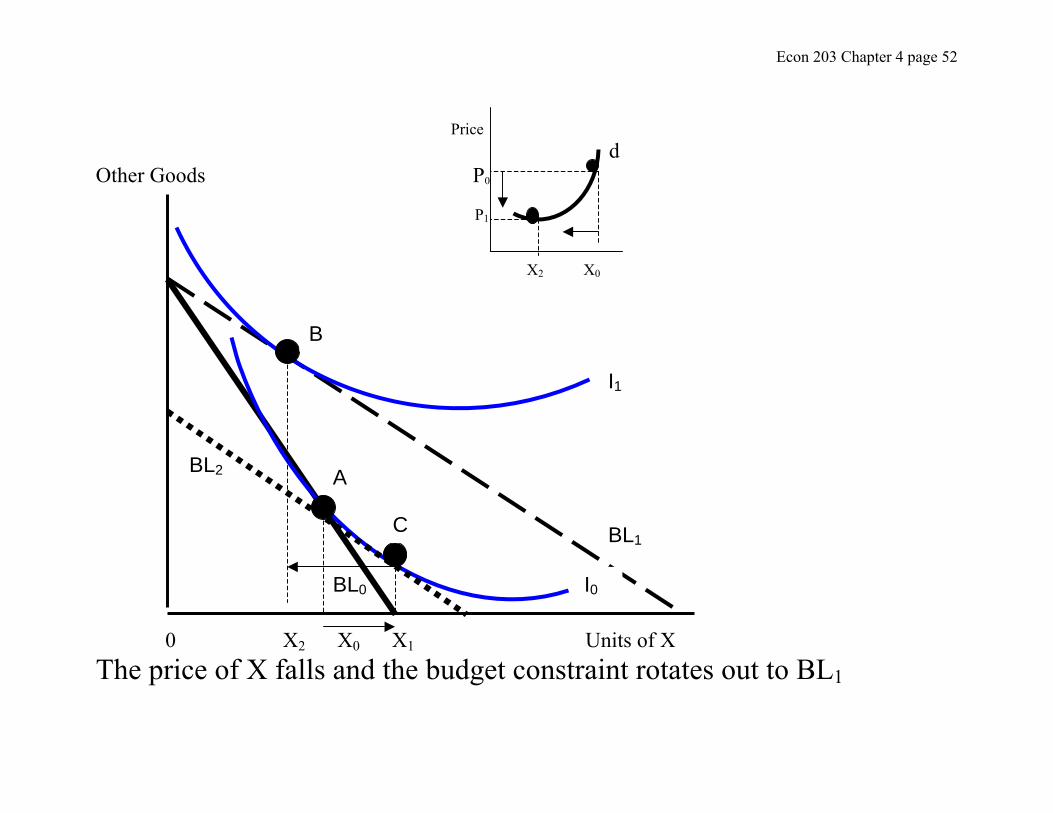
Price d Other Goods P0 P1 X2 X0 0 X2 X0 X1 Units of X The price of X falls and the budget constraint rotates out to BL1

A

BL0

BL2

B

C

I1

I0

BL1


The total change from the decrease in the price of good X can be separated into two components: The substitution effect is X1 - X0. (Opposite direction to the price change.) The income effect is X1-X2. (Same direction as the price change.)

The net effect is a fall in the quantity demanded due to a fall in price.


The consumer’s demand function has a positive slope. This is because the income effect overwhelms the substitution effect. When this occurs, we refer to this good as a Giffen good.


2) The Substitution Effect Overwhelms the Income Effect Price Other Goods P0 P1 X0 X2 0 X0 X0 X1 Units of X

A

BL0

BL2

B

C

I1

I0

BL1

d


In this case, the demand curve will have a negative slope: The price of X decreases. The substitution effect equals X1-X0. The income effect equals X2-X1. Hence, with a decrease in the price of X, the quantity of X demanded increases because the substitution effect overwhelms the income effect.


The Slope of the Demand Function The consumer’s demand function represents the relationship between the quantity demanded and the price of the good with income and other prices held constant; X=d(P) (Individual Demand Function)

The slope of the demand function is ΔΔXP and depends on the

size of the substitution and income effects. So, in order to determine whether a price change will result in a large or small change in the quantity demanded, we need to determine the size of the income or substitution effect.


Recall, the substitution effect measures the change in the quantity demanded due to a price change holding utility constant. This can be expressed as:

ΔΔXP U C= .

ΔΔXP can be determined by measuring how the quantity

demanded changes along an indifference curve as the relative price of the good X changes. This quantity will always be negative since the consumer demands more units of a good when its price decreases.


The slope of the demand curve also depends on the income effect. So, when will this effect be large? It depends on two factors: 1) The amount of income that is freed up when the price of

the good falls. 2) The number of units the consumer now demands since

income has increased.


The income that becomes available per dollar change in price depends on the number of units the consumer is presently consuming. When the price of the good falls, the amount of income available to spend on goods is equal to:

Δ ΔM P X= −( ) Looking at this expression, the greater is the change in income the larger is the amount of X the consumer is currently consuming. The change in income per dollar decrease in price equals: ΔΔMP

X⎛⎝⎜

⎞⎠⎟= − .


ΔΔ

XM

⎛⎝⎜

⎞⎠⎟ equals the increase in the quantity demanded of X per dollar

increase in income. Thus, the change in the quantity demanded due to the income

effect is − • ⎛⎝⎜

⎞⎠⎟

X XMΔΔ

Recall, the change in the quantity demanded due to a price change is the sum of the changes caused by the substitution effect and the income effect.


The slope of the consumer’s demand function can be expressed as: ΔΔ

ΔΔ

ΔΔ

XP

XP

X XMU c

⎛⎝⎜

⎞⎠⎟= − ⎛

⎝⎜⎞⎠⎟=

Slutsky Equation Slutsky Equation: the slope of the demand function equals the sum of the substitution and income effects. The sign of the substitution effect is always negative.


When the income effect is negative, the slope of the demand curve is negative due to the fact that the substitution effect is always negative. If the good is a normal good, the income effect is also negative. ►The demand function will have a negative slope. ☺ If the good is an inferior good, the income effect will be positive and the slope of the demand curve can be either positive or negative.


Consumer Surplus Objective: to demonstrate how consumer surplus is derived from the consumer’s demand function.

Consumer surplus is the difference between the maximum amount the purchaser would pay to consume a given quantity of a good and the actual amount paid. It is assumed that the consumer receives a surplus by consuming the good and is willing to pay even more than go without the good.


Marginal Value: is the most that a consumer is willing to pay for each additional unit of a good. A consumer that maximizes consumer surplus will determine the quantity to buy such that marginal value equals price. Example: Muffins

$3.50 $2.75 $2.10 $1.75 $1.50 $0.75

Price or Marginal Value

Consumer keeps buying a unit until consumer surplus equals zero.Stops buying when: $P > Marginal value

0 1 2 3 4 5 Muffins per day


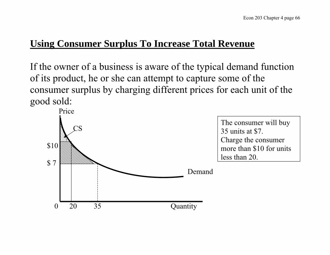
Using Consumer Surplus To Increase Total Revenue If the owner of a business is aware of the typical demand function of its product, he or she can attempt to capture some of the consumer surplus by charging different prices for each unit of the good sold: Price CS $10 $ 7 Demand 0 20 35 Quantity

The consumer will buy 35 units at $7. Charge the consumer more than $10 for units less than 20.


Discriminatory pricing! Transfer of surplus from consumer to producer! ☺ ☺ ☺ ☺ ☺ ☺ ☺ What About Pricing Policies that generate a loss of consumer surplus? Some policies are designed to protect the producer, but at the expense of the consumer.


By increasing price and restricting output, these policies harm the consumer and generate a loss known as a dead-weight-loss. Dead-weight-loss: represents the decrease in consumer surplus that is not transferred to some other group. Price $11 Dead weight loss $ 7 Demand 0 5 15 Quantity

Monopoly: Restrict output and charge higher prices. → Not good for the consumer.

chapter 4: individual and market demand - university …web.uvic.ca/~okhan/ch 4 individual and...

Documents