chapter 4 duality - stanford universityashishg/msande111/notes/chapter4.pdf · chapter 4 duality...

Chapter 4

Duality

Given any linear program, there is another related linear program called thedual. In this chapter, we will develop an understanding of the dual linearprogram. This understanding translates to important insights about manyoptimization problems and algorithms. We begin in the next section byexploring the main concepts of duality through the simple graphical exampleof building cars and trucks that was introduced in Section 3.1.1. Then, wewill develop the theory of duality in greater generality and explore moresophisticated applications.

4.1 A Graphical Example

Recall the linear program from Section 3.1.1, which determines the optimalnumbers of cars and trucks to build in light of capacity constraints. There aretwo decision variables: the number of cars x1 in thousands and the numberof trucks x2 in thousands. The linear program is given by

maximize 3x1 + 2.5x2 (profit in thousands of dollars)subject to 4.44x1 ≤ 100 (car assembly capacity)

6.67x2 ≤ 100 (truck assembly capacity)4x1 + 2.86x2 ≤ 100 (metal stamping capacity)3x1 + 6x2 ≤ 100 (engine assembly capacity)x ≥ 0 (nonnegative production).

The optimal solution is given approximately by x1 = 20.4 and x2 = 6.5,generating a profit of about $77.3 million. The constraints, feasible region,and optimal solution are illustrated in Figure 4.1.

83

84

10 20 30 40

10

20

30

40 truck assemblyengine

assembly

metal

stamping

car assembly

feasible solutions

trucks produced (thousands)

cars

pro

duced (

thousands)

optimal

solution

Figure 4.1: The constraints, feasible region, and optimal solution of the linearprogram associated with building cars and trucks.

Written in matrix notation, the linear program becomes

maximize cT xsubject to Ax ≤ b

x ≥ 0,

where

c =

[3

2.5

], A =

4.44 00 6.674 2.863 6

and b =

100100100100

.

The optimal solution of our problem is a basic feasible solution. Sincethere are two decision variables, each basic feasible solution is characterizedby a set of two linearly independent binding constraints. At the optimalsolution, the two binding constraints are those associated with metal stamp-ing and engine assembly capacity. Hence, the optimal solution is the uniquesolution to a pair of linear equations:

4x1 + 2.86x2 = 100 (metal stamping capacity is binding)3x1 + 6x2 = 100 (engine assembly capacity is binding).

In matrix form, these equations can be written as Ax = b, where

A =

[(A3∗)

T

(A4∗)T

]and b =

[b3

b4

].

c©Benjamin Van Roy and Kahn Mason 85

Note that the matrix A has full rank. Therefore, it has an inverse A−1

.Through some calculations, we get (approximately)

A−1

=

[0.389 −0.185−0.195 0.259

].

The optimal solution of the linear program is given by x = A−1

b, and there-

fore, the optimal profit is cT A−1

b = 77.3.

4.1.1 Sensitivity Analysis

Suppose we wish to increase profit by expanding manufacturing capacities.In such a situation, it is useful to think of profit as a function of a vector∆ ∈ <4 of changes to capacity. We denote this profit by z(∆), defined to bethe maximal objective value associated with the linear program

maximize cT xsubject to Ax ≤ b + ∆

x ≥ 0.(4.1)

Hence, the maximal profit in our original linear program is equal to z(0). Inthis section, we will examine how incremental changes in capacities influencethe optimal profit z(∆). The study of such changes is called sensitivityanalysis.

Consider a situation where the metal stamping and engine assembly ca-pacity constraints are binding at the optimal solution to the linear program

(4.1). Then, this optimal solution must be given by x = A−1

(b+∆), and the

optimal profit must be z(∆) = cT A−1

(b + ∆), where

∆ =

[∆3

∆4

].

Furthermore, the difference in profit is z(∆)− z(0) = cT A−1

∆.This matrix equation provides a way to gauge the impact of changes in

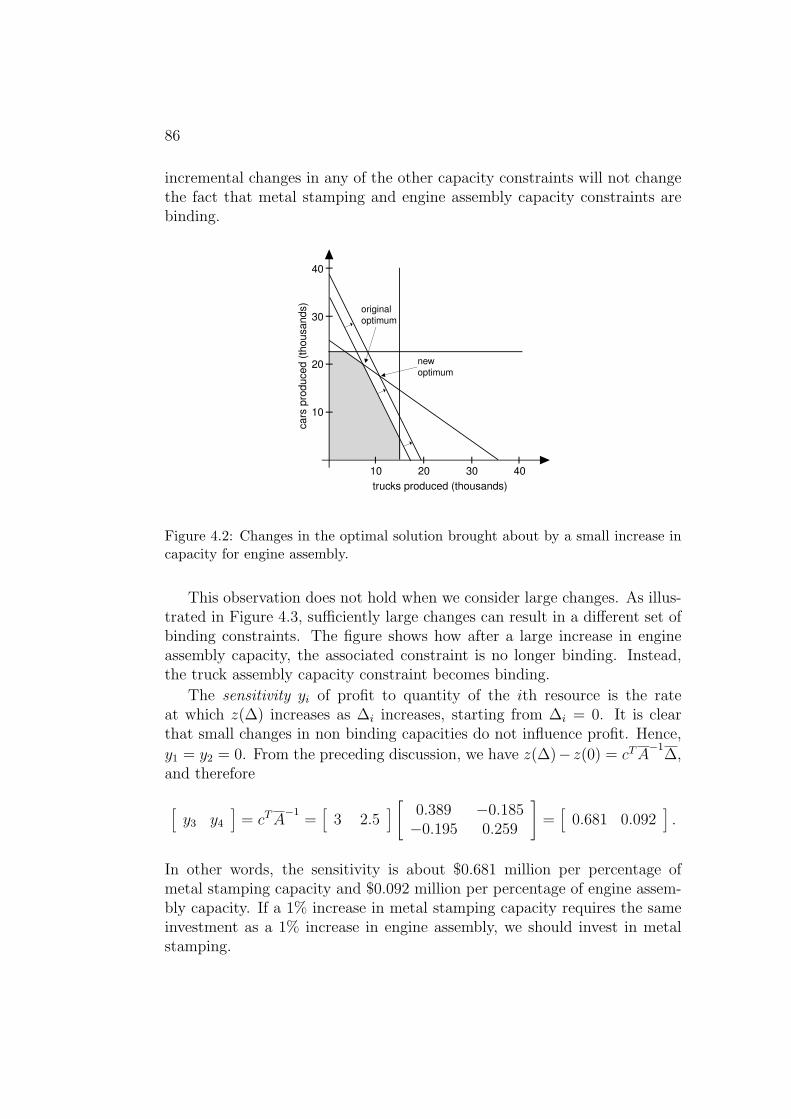
capacities on optimal profit in the event that the set of binding constraintsdoes not change. It turns out that this also gives us the information requiredto conduct sensitivity analysis. This is because small changes in capacitieswill not change which constraints are binding. To understand why, considerthe illustration in Figure 4.2, where the engine assembly capacity is increasedby a small amount. Clearly, the new optimal solution is still at the inter-section where metal stamping and engine assembly capacity constraints arebinding. Similarly, though not illustrated in the figure, one can easily see that

86

incremental changes in any of the other capacity constraints will not changethe fact that metal stamping and engine assembly capacity constraints arebinding.

10 20 30 40

10

20

30

40


cars

pro

duced (

thousands)

original

optimum

new

optimum

Figure 4.2: Changes in the optimal solution brought about by a small increase incapacity for engine assembly.

This observation does not hold when we consider large changes. As illus-trated in Figure 4.3, sufficiently large changes can result in a different set ofbinding constraints. The figure shows how after a large increase in engineassembly capacity, the associated constraint is no longer binding. Instead,the truck assembly capacity constraint becomes binding.

The sensitivity yi of profit to quantity of the ith resource is the rateat which z(∆) increases as ∆i increases, starting from ∆i = 0. It is clearthat small changes in non binding capacities do not influence profit. Hence,

y1 = y2 = 0. From the preceding discussion, we have z(∆)− z(0) = cT A−1

∆,and therefore

[y3 y4

]= cT A

−1=

[3 2.5

] [0.389 −0.185−0.195 0.259

]=

[0.681 0.092

].

In other words, the sensitivity is about $0.681 million per percentage ofmetal stamping capacity and $0.092 million per percentage of engine assem-bly capacity. If a 1% increase in metal stamping capacity requires the sameinvestment as a 1% increase in engine assembly, we should invest in metalstamping.


10 20 30 40

10

20

30

40


cars

pro

duced (

thousands)

original

optimum

new

optimum

Figure 4.3: Changes in the optimal solution brought about by a large increase incapacity for engine assembly.

4.1.2 Shadow Prices and Valuation of the Firm

The sensitivities of profit to resource quantities are commonly called shadowprices. Each ith resource has a shadow price yi. In our example of buildingcars and trucks, shadow prices for car and truck assembly capacity are zero.Shadow prices of engine assembly and metal stamping capacity, on the otherhand, are $0.092 and $0.681 million per percent. Based on the discussionin the previous section, if the metal stamping and engine assembly capacityconstraints remain binding when resource quantities are set at b + ∆, theoptimal profit is given by z(∆) = z(0) + yT ∆.

A shadow price represents the maximal price at which we should be willingto buy additional units of a resource. It also represents the minimal price atwhich we should be willing to sell units of the resource. A shadow price mighttherefore be thought of as the value per unit of a resource. Remarkably, if wecompute the value of our entire stock of resources based on shadow prices,we get our optimal profit! For instance, in our example of building cars andtrucks, we have

0.092× 100 + 0.681× 100 = 77.3.

As we will now explain, this is not just a coincidence but reflects a funda-mental property of shadow prices.

From the discussion above we know that as long as the metal stampingand engine assembly constraints are binding, that z(∆) = z(0) + yT ∆. Ifwe let ∆ = −b, then the resulting linear program has 0 capacity at each

88

plant, so the optimal solution is 0, with associated profit of 0. Moreover,both the metal stamping and engine assembly constraints are still binding.This means that 0 = z(−b) = z(0) + yT (−b). Rearranging this gives thatz(0) = yT b. This is a remarkable fundamental result: the net value of ourcurrent resources, valued at their shadow prices, is equal to the maximalprofit that we can obtain through operation of the firm – i.e., the value ofthe firm.

4.1.3 The Dual Linear Program

Shadow prices solve another linear program, called the dual. In order todistinguish it from the dual, the original linear program of interest – in thiscase, the one involving decisions on quantities of cars and trucks to build inorder to maximize profit – is called the primal. We now formulate the dual.

To understand the dual, consider a situation where we are managing thefirm but do not know linear programming. Therefore, we do not know exactlywhat the optimal decisions or optimal profit are. Company X approaches usand expresses a desire to purchase capacity at our factories. We enter into anegotiation over the prices y ∈ <4 that we should charge per percentage ofcapacity at each of our four factories.

To have any chance of interesting us, the prices must be nonnegative:y ≥ 0. We also argue that there are fixed bundles of capacity that we can useto manufacture profitable products, and the prices y must be such that sellingsuch a bundle would generate at least as much money as manufacturing theproduct. In other words, we impose requirements that

4.44y1 + 4y3 + 3y4 ≥ 3 and 6.67y2 + 2.86y3 + 6y4 ≥ 2.5.

The first constraint ensures that selling a bundle of capacity that could beused to produce a car is at least as profitable as producing the car. Thesecond constraint is the analog associated with production of trucks.

Given our requirements, Company X solves a linear program to determineprices that minimize the amount it would have to pay to purchase all of ourcapacity:

minimize 100y1 + 100y2 + 100y3 + 100y4 (cost of capacity)subject to 4.44y1 + 4y3 + 3y4 ≥ 3 (car production)

6.67y2 + 2.86y3 + 6y4 ≥ 2.5 (truck production)y ≥ 0 (nonnegative prices).


In matrix notation, we have

minimize bT ysubject to AT y ≥ c

y ≥ 0.

The optimal solution to this linear program is

y =

00

0.0920.681

,

and the minimal value of the objective function is 77.3. Remarkably, we haverecovered the shadow prices and the optimal profit!

It is not a coincidence that the minimal cost in the dual equals the optimalprofit in the primal and that the optimal solution of the dual is the vector ofshadow prices – these are fundamental relations between the primal and thedual. We offer an intuitive explanation now and a more in-depth analysis inthe next section.

The constraints ensure that we receive at least as much money from sellingas we would from manufacturing. Therefore, it seems clear that the minimalcost in the dual is at least as large as the maximal profit in the primal. Thisfact is known as weak duality. Another result, referred to as strong duality,asserts that the minimal cost in the dual equals the maximal profit in theprimal. This is not obvious. It is motivated to some extent, though, by thefact that Company X is trying to get the best deal it can. It is natural tothink that if Company X negotiates effectively, it should be able to acquireall our resources for an amount of money equal that we would obtain as profitfrom manufacturing. This would imply strong duality.

Why, now, should an optimal solution to the dual provide shadow prices?To see this, consider changing the resource quantities by a small amount∆ ∈ <4. Then, the primal and dual become

maximize cT x minimize (b + ∆)T ysubject to Ax ≤ b + ∆ and subject to AT y ≥ c

x ≥ 0 y ≥ 0.

The maximal profit in the primal and the minimal cost in the dual are bothequal to z(∆). Suppose that the optimal solution to the dual is unique – asis the case in our example of building cars and trucks. Then, for sufficientlysmall ∆, the optimal solution to the dual should not change, and thereforethe optimal profit should change by z(∆)−z(0) = (b+∆)T y−bT y = ∆T y. Itfollows that the optimal solution to the dual is the vector of shadow prices.

90

4.2 Duality Theory

In this section, we develop weak and strong duality in general mathematicalterms. This development involves intriguing geometric arguments. Devel-oping intuition about the geometry of duality is often helpful in generatinguseful insights about optimization problem.

Duality theory applies to general linear programs, that can involve greater-than, less-than, and equality constraints. However, to keep things simple, wewill only study in this section linear programs that are in symmetric form.Such linear programs take the form:


x ≥ 0.

for some matrix A ∈ <M×N and vectors b ∈ <M and c ∈ <N . The decisionvariables – called the primal variables – make up a vector x ∈ <N . As wewill discuss later in the chapter, general linear programs can be converted tosymmetric form, so our development of duality theory in this context alsoapplies to general linear programs.

The dual of a symmetric form linear program takes the form

minimize bT ysubject to AT y ≥ c

y ≥ 0.

The decision variables – called the dual variables – form a vector y ∈ <M .Note that each decision variable in the primal problem corresponds to a

constraint in the dual problem, and each constraint in the primal problemcorresponds to a variable in the dual problem.

4.2.1 Weak Duality

Suppose that x is a feasible solution of the primal and y is a feasible solutionof the dual. Then, Ax ≤ b, yT A ≥ cT , x ≥ 0, and y ≥ 0. It follows thatyT Ax ≥ cT x and yT Ax ≤ yT b. Hence, cT x ≤ bT y. This is the weak dualitytheorem, which we state below:

Theorem 4.2.1. (Weak Duality) For any feasible solutions x and y toprimal and dual linear programs, cT x ≤ bT y.

The following theorem states one immediate implication of weak duality.


Theorem 4.2.2. (Certificate of Optimality) If x and y are feasible so-lutions of the primal and dual and cT x = bT y, then x and y must be optimalsolutions to the primal and dual.

There is another interesting consequence of weak duality that relates in-finiteness of profit/cost in the primal/dual with feasibility of the dual/primal,as we now explain. Let y be a feasible solution of the dual. By weak duality,we have cT x ≤ bT y for all feasible x. If the optimal profit in the primal is ∞,then ∞ ≤ bT y. This is not possible, so the dual cannot have a feasible so-lution. The following theorem captures this fact, together with its converse,which can be established via a symmetric argument.

Theorem 4.2.3. (Infiniteness and Feasibility in Duality) If the optimalprofit in the primal is ∞, then the dual must be infeasible. If the optimal costin the dual is −∞, then the primal must be infeasible.

4.2.2 Strong Duality

Theorem 4.2.2 asserts that if x and y are feasible solutions of the primal anddual and cT x = bT y, then x and y must be optimal solutions of the primaland dual. This does not imply that there are feasible solutions x and y suchthat cT x = bT y. However the strong duality guarantees this.

Theorem 4.2.4. (Strong Duality) The dual has an optimal solution ifand only if the primal does. If x∗ and y∗ are optimal solutions to the primaland dual, then cT x∗ = bT y∗.

Note that here, and throughout the book, when we refer to an optimalsolution, it is implicitly assumed to be finite. If the optimal value can getarbitrarily large, we say the objective is unbounded. There are two slightlydifferent sorts of unboundedness we discuss, subtly different. In the first,the feasible region is unbounded, and in this situation we say the problem isunbounded. In the second, the objective function can get arbitrarily large,and we say that the objective value is unbounded. Note that the second sortof unboundedness implies the first.

In order to prove the Strong Duality Theorem, we first have an aside, anddiscuss optimality of slightly more general functions.

4.2.3 First Order Necessary Conditions

It is possible to establish the Strong Duality Theorem directly, but the KKTconditions (given later in this section) are useful in their own right, andstrong duality is an immediate consequence.

92

Before given the KKT conditions, we digress still more, and talk aboutconvex sets and hyperplanes. Given two sets, U and V , we say that a hyper-plane H separates U and V if all of U is on one side of the hyperplane, andall of V is on the other side. In other words, if H is given by {x|aT x = b},then H separates <N into two sets, H+ = {x|aT x ≥ b} and H− {x|aT x ≤ b}.H separates U and V if U is contained in H+ and V is contained in H− orvice versa.

Theorem 4.2.5. (Separating Hyperplane) Let U and V be two disjointconvex sets. Then, there exists a hyperplane separating U and V .

“Picture Proof:” Let δ = infu∈U,v∈V ‖u − v‖ We will demonstrate theresult only for the case where δ > 0 and there is a u ∈ U and v ∈ V with‖u− v‖ = δ. This case is all that will be needed to cover all the applicationswe will use of the theorem, and the full result is beyond the scope of thisbook.

Take u ∈ U and v ∈ V with ‖u − v‖ = δ. Let H be the hyperplanethrough v that is perpendicular to u − v. We claim that H is a separatinghyperplane for U and V .

Suppose this were not the case. Then, without loss of generality, we canassume that v = 0 (we can translate every point by −v). The means thatH will be given by {x|uT x = 0}. Note that 0 ∈ H−. Suppose not all of Uis in H+. Then there would be some v ∈ U with uT v < 0. If d = v − u andα = −uT d

dT d∈ (0, 1), and let w = u + αd = αv + (1 − α)u. w must be in U

because it is a convex combination of things in U , and the length of w is

wT w = (u + αd)T (u + αd)

= uT u + 2αuT d + α2dT d

= uT u + αdT d(2uT d

dT d+ α)

< uT u

because uT d < 0. This contradicts the fact that u was the point in U closestto the origin. Thus, all of U is in H+. A similar argument shows that eachpoint of V must lie in H− or else the convexity of V would generate a pointcloser to u than 0, and so H is a separating hyperplane for U and V .

As discussed in the above proof, we will only be needing a restricted formof the separating hyperplane here. In particular, the following result whichfollows from the fact that polyhedra are closed (they are the intersection of


closed half spaces), and for any point x and any closed set P , there is a pointin P that is closest to x.1

Corollary 4.2.1. Separating Hyperplane Theorem If P is a polyhedron,and x is a point distinct from P , then there is a vector s such that sT x < sT pfor all p ∈ P .

A corollary of separating hyperplanes is Farkas’ lemma.

Lemma 4.2.1. Farkas’ Lemma For any A ∈ <M×N and b ∈ <M , exactlyone of the following two alternatives holds:(a) There exists a vector x ∈ <N such that x ≥ 0, Ax = b.(b) There exists a vector y ∈ <M such that bT y < 0 and AT y ≥ 0.

Proof:

If (a) and (b) are both true, then 0 > bT y = yT b = yT Ax = xT AT y ≥ 0,which is a contradiction. This means that (a) being true makes (b) false.

Suppose that (a) is false, then b is not in the polyhedron P = {Ax, x ≥0}2. Let y be the vector guaranteed by the separating hyperplane theorem.This means that yT b < yT p for all p ∈ P . 0 is in P , so this means thatbT y = yT b < 0. Suppose yT Aj∗ < 0 for some j. Then for some α we musthave yT (αAj∗) < yT b violating the fact that αAj∗ is in P . Thus yT Aj∗ ≥ 0for each j, or AT y ≥ 0 so that (b) is true.

We can now give the KKT conditions. Note that these conditions arenecessary, but not sufficient for a maximizer. There is a slight technicalcondition on the maximizing point, it needs to be regular. A regular pointis one where if all active constraints are linearized (that is, replaced withtangent hyperplanes), the set of feasible directions remains the same.3. Thisrules out some extremely rare coincidences of constraints, and note that inlinear systems every point is regular.

That caveat aside, here are the KKT conditions.

Theorem 4.2.6. Suppose that f, g1, g2, . . . gM are differentiable functionsfrom <N into <. Let x be the point that maximizes f subject to gi(x) ≤ 0 foreach i, and assume the first k constraints are active and x is regular. Thenthere exists y1, . . . , yk ≥ 0 such that ∇f(x) = y1∇g1(x) + . . . + yk∇gk(x).

1Despite being obvious if drawn, this result is typically established using the fact thatdistance is a continuous function and applying Weierstrass’ theorem.

2To see that P is a polyhedron, it can also be written as {y|y = Ax, x ≥ 0}.3If there is a feasible curve from x whose initial direction is d, then d is a feasible

direction.

94

Proof: Let c = ∇f(x). The directional derivative of f in the directionof unit vector z is zT c. Thus, every feasible direction z must have zT c ≤ 0.Let A ∈ <k×N be the matrix whose ith row is (∇gi(x))T . Then a directionz is feasible if Az ≤ 0. Thus, there is no z with Az ≤ 0 and cT z > 0.From Farkas’ lemma, we can now say that there is a y such that y ≥ 0 andAT y = c, which is the statement of the theorem.

Note that the conditions describe∇f as a combination of active constraintgradients only. Another way of stating the conditions is to say that ∇f =y1∇g1(x) + . . . + yn∇gn(x) where yigi(x) = 0. Now the sum is over allconstraints (not just the active ones), but the second condition says that thecoefficients of non-active constraints must be 0. The condition yigi(x) = 0 iscalled a complementarity condition, and is another certificate of optimality.

The Strong Duality Theorem is an application of the KKT conditions tothe particular case where each of the functions being considered is linear.

Proof of strong duality: The primal problem is given by


x ≥ 0.

Letting f(x) = cT x, g1(x) = (Ax − b)1, . . . , gM(x) = (Ax − b)M , gM+1(x) =

−x1, . . . , gM+N(x) = −xN , we see that the primal is equivalent to

maximize f(x)subject to g(x) ≤ 0.

Note that ∇g(x∗) = c, ∇gk(x) = Ak∗ for k = 1, . . . ,M , and ∇gk(x) = −ek

for k = M + 1, . . . ,M + N .Suppose x∗ is an optimal solution. The KKT conditions ensure existence

y ∈ <M and z ∈ <N such that y ≥ 0, z ≥ 0, c = AT y− z, and (Ax∗− b)T y−(x∗)T z = 0. It follows that AT y ≥ c and bT y = (AT y − z)T x∗ = cT x. Theresult follows.

4.2.4 Complementary Slackness

Recall that if x∗ and y∗ are optimal solutions to primal and dual linear pro-grams, each dual variable y∗i can be viewed as the sensitivity of the objectivevalue to the value of bi. If the constraint AT

i∗x ≤ bi is not binding, the objec-tive value should not be sensitive to the value of bi, and therefore, y∗i shouldbe equal to zero. The fact that this is true for every i can be expressedconcisely in terms of an equation: (b−Ax∗)T y∗ = 0; since all components ofboth b−Ax∗ and y∗ are nonnegative, the only way the inner product can be


equal to 0 is if, for each ith component, either ATi∗x = bi or yi = 0 . Similarly,

since the primal is the dual of the dual, each x∗j represents sensitivity of theobjective value to cj, and we have (AT y∗ − c)T x∗ = 0.

The preceding discussion suggests that, for any optimal solutions x∗ andy∗ to the primal and dual, (b−Ax∗)T y∗ = 0 and (AT y∗−c)T x∗ = 0. Interest-ingly, in addition to this statement, the converse is true: for any feasible solu-tions x and y to the primal and dual, if (b−Ax)T y = 0 and (AT y− c)T x = 0then x and y are optimal solutions to the primal and dual. These factsare immediate consequences of duality theory. They are captured by thecomplementary slackness theorem, which we now state and prove.

Theorem 4.2.7. Complementary Slackness) Let x and y be feasible so-lutions to symmetric form primal and dual linear programs. Then, x and yare optimal solutions to the primal and dual if and only if (b − Ax)T y = 0and (AT y − c)T x = 0.

Proof: Feasibility implies that (b − Ax)T y ≥ 0 and (AT y − c)T x ≥ 0.Further, if x and y are optimal,

(AT y − c)T x + (b− Ax)T y = bT y − cT x = 0,

by strong duality (Theorem 4.2.4). Hence, if x and y are optimal, (b −Ax)T y = 0 and (AT y − c)T x = 0.

For the converse, suppose that x and y are feasible and that (b−Ax)T y = 0and (AT y − c)T x = 0. Then,

0 = (AT y − c)T x + (b− Ax)T y = bT y − cT x,

which provides a certificate of optimality (Theorem 4.2.2).There are many interesting consequences to complementary slackness.

We will consider in Section 4.5 one application involving allocation of a laborforce among interdependent production processes.

4.3 Duals of General Linear Programs

For a linear program that isn’t in the symmetric form we can still constructthe dual problem. To do this, you can transform the linear program to sym-metric form, and then construct the dual from that. Alternatively, you canapply the KKT conditions directly. Either approach results in an equivalentproblem.

For example, suppose the linear program is minimize cT x subject to Ax ≤b, x ≥ 0. Then because minimizing cT x is the same as maximizing −cT x =

96

(−c)T x, the linear program is the same as maximize (−c)T x subject to Ax ≤b, x ≥ 0.

The modifications needed are summarized below.

• If the objective function, cT x is minimized rather than maximized, thenreplace c by −c.

• If a constraint is a greater than constraint, aT x ≥ β, then take thenegative of the constraint to get (−a)T x ≤ −β.

• If a constraint is an equality constraint, aT x = β, then treat it as agreater than constraint and a less than constraint to get aT x ≤ β and(−a)T x ≤ −β.

• If x is not constrained to be positive, then replace x by x+ and x−, therex+ represents the positive part of x, and x− represents the negativepart of x, just like the arbitrage example of the previous chapter.

As an example, suppose the linear program is

minimize cT xsubject to A1x ≤ b1

A2x ≥ b2

A3x = b3

Then rearranging into symmetric form would give

maximize (−c)T x+ + cT x−

subject to A1x+ − A1x− ≤ b1

(−A2)x+ + A2x− ≤ −b2

A3x+ − A3x− ≤ b3

(−A3)x+ + A3x− ≤ −b3

x+, x− ≥ 0

Note that if x+, x− is a solution, then so is x+ + y, x− + y for any y ≥ 0.However, if y 6= 0, then this will not represent a vertex.

Taking the dual of the above linear program gives

minimize (b1)T y1 − (b2)T y2 + (b3)T y3 − (b3)T y4

subject to (A1)T y1 − (A2)T y2 + (A3)T y3 − (A3)T y4 ≥ −c(−A1)T y1 + (A2)T y2 − (A3)T y3 + (A3)T y4 ≥ cy1, y2, y3, y4 ≥ 0


Notice that y3 and y4 are exactly what they would have been if one hadreplaced an unconstrained y with y3 = y+ and y4 = y−. Thus, writingy = y3 − y4, we can rewrite the dual as

minimize (b1)T y1 − (b2)T y2 + (b3)T ysubject to (A1)T y1 − (A2)T y2 + (A3)T y ≥ −c

(−A1)T y1 + (A2)T y2 − (A3)T y ≥ cy1, y2 ≥ 0

The fact that equality constraints in the primal correspond to uncon-strained variables in the dual is but one aspect that can be observed bylooking at the above dual. Other features are summarized in the table be-low, which describes how to take the dual of a general linear program.

PRIMAL maximize minimize DUAL≤ bi ≥ 0

constraints ≥ bi ≤ 0 variables= bi unconstrained≥ 0 ≥ cj

variables ≤ 0 ≤ cj constraintsunconstrained = cj

Note, using the rules in the above table, the dual of

minimize cT xsubject to A1x ≤ b1

A2x ≥ b2

A3x = b3

becomes

maximize (b1)T y1 + (b2)T y2 + (b3)T y3

subject to (A1)T y1 + (A2)T y2 + (A3)T y3 = cy1 ≤ 0y2 ≥ 0

Since the dual of the dual is the primal, reorganizing the above table yieldsan alternative procedure for converting primals that involve minimization totheir duals.

98

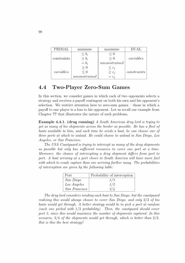
PRIMAL minimize maximize DUAL≤ bi ≤ 0

constraints ≥ bi ≥ 0 variables= bi unconstrained≥ 0 ≤ cj

variables ≤ 0 ≥ cj constraintsunconstrained = cj

4.4 Two-Player Zero-Sum Games

In this section, we consider games in which each of two opponents selects astrategy and receives a payoff contingent on both his own and his opponent’sselection. We restrict attention here to zero-sum games – those in which apayoff to one player is a loss to his opponent. Let us recall our example fromChapter ?? that illustrates the nature of such problems.

Example 4.4.1. (drug running) A South American drug lord is trying toget as many of his shipments across the border as possible. He has a fleet ofboats available to him, and each time he sends a boat, he can choose one ofthree ports at which to unload. He could choose to unload in San Diego, LosAngeles, or San Francisco.

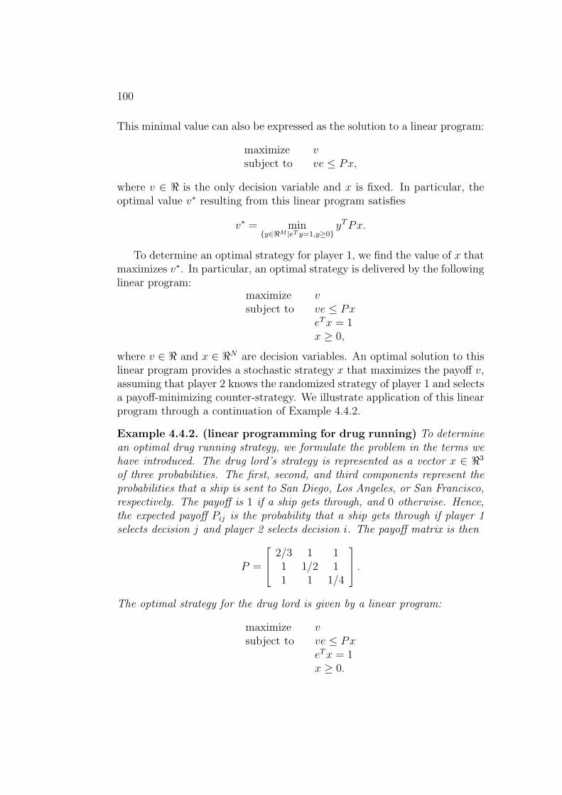
The USA Coastguard is trying to intercept as many of the drug shipmentsas possible but only has sufficient resources to cover one port at a time.Moreover, the chance of intercepting a drug shipment differs from port toport. A boat arriving at a port closer to South America will have more fuelwith which to evade capture than one arriving farther away. The probabilitiesof interception are given by the following table:

Port Probability of interceptionSan Diego 1/3Los Angeles 1/2San Francisco 3/4

The drug lord considers sending each boat to San Diego, but the coastguardrealizing this would always choose to cover San Diego, and only 2/3 of hisboats would get through. A better strategy would be to pick a port at random(each one picked with 1/3 probability). Then, the coastguard should coverport 3, since this would maximize the number of shipments captured. In thisscenario, 3/4 of the shipments would get through, which is better than 2/3.But is this the best strategy?


Clearly, the drug lord should consider randomized strategies. But whatshould he optimize? We consider as an objective maximizing the probabilitythat a ship gets through, assuming that the Coastguard knows the drug lord’schoice of randomized strategy. We now formalize this solution concept forgeneral two-person zero-sum games, of which our example is a special case.

Consider a game with two players: player 1 and player 2. Suppose thereare N alternative decisions available to player 1 and M available to player2. If player 1 selects decision j ∈ {1, . . . , N} and player 2 selects decisioni ∈ {1, . . . ,M}, there is an expected payoff of Pij to be awarded to player1 at the expense of player 2. Player 1 wishes to maximize expected payoff,whereas player 2 wishes to minimize it. We represent expected payoffs forall possible decision pairs as a matrix P ∈ <M×N .

A randomized strategy is a vector of probabilities, each associated witha particular decision. Hence, a randomized strategy for player 1 is a vectorx ∈ <N with eT x = 1 and x ≥ 0, while a randomized strategy for player 2 is avector y ∈ <M with eT y = 1 and y ≥ 0. Each xj is the probability that player1 selects decision j, and each yi is the probability that player 2 selects decisioni. Hence, if the players apply randomized strategies x and y, the probabilityof payoff Pij is yixj and the expected payoff is

∑Mi=1

∑Nj=1 yixjPij = yT Px.

How should player 1 select a randomized policy? As a solution concept,we consider selection of a strategy that maximizes expected payoff, assumingthat player 2 knows the strategy selected by player 1. One way to write thisis as

max{x∈<N |eT x=1,x≥0}

min{y∈<M |eT y=1,y≥0}

yT Px.

Here, y is chosen with knowledge of x, and x is chosen to maximize theworst-case payoff. We will now show how this optimization problem can besolved as a linear program.

First, consider the problem of optimizing y given x. This amounts to alinear program:

minimize (Px)T ysubject to eT y = 1

y ≥ 0.

It is easy to see that the basic feasible solutions of this linear program aregiven by e1, . . . , eM , where each ei is the vector with all components equal to0 except for the ith, which is equal to 1. It follows that


yT Px = mini∈{1,...,M}

(Px)i.

100

This minimal value can also be expressed as the solution to a linear program:

maximize vsubject to ve ≤ Px,

where v ∈ < is the only decision variable and x is fixed. In particular, theoptimal value v∗ resulting from this linear program satisfies

v∗ = min{y∈<M |eT y=1,y≥0}

yT Px.

To determine an optimal strategy for player 1, we find the value of x thatmaximizes v∗. In particular, an optimal strategy is delivered by the followinglinear program:

maximize vsubject to ve ≤ Px

eT x = 1x ≥ 0,

where v ∈ < and x ∈ <N are decision variables. An optimal solution to thislinear program provides a stochastic strategy x that maximizes the payoff v,assuming that player 2 knows the randomized strategy of player 1 and selectsa payoff-minimizing counter-strategy. We illustrate application of this linearprogram through a continuation of Example 4.4.2.

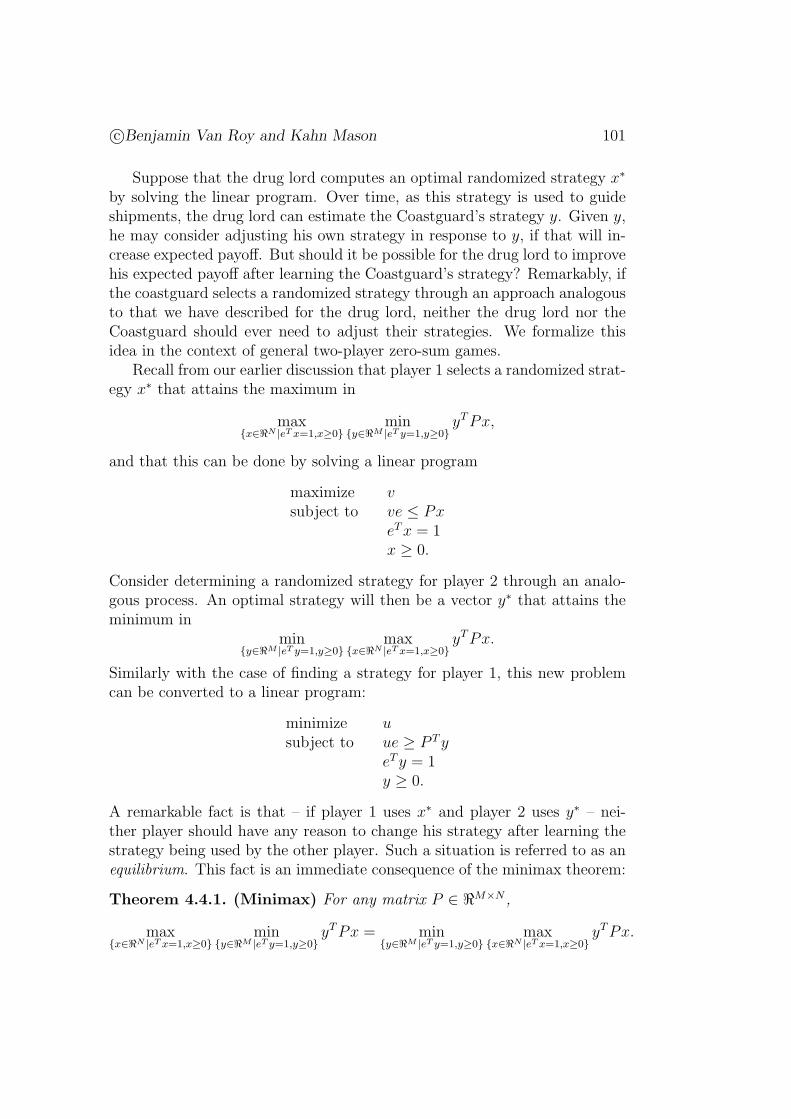
Example 4.4.2. (linear programming for drug running) To determinean optimal drug running strategy, we formulate the problem in the terms wehave introduced. The drug lord’s strategy is represented as a vector x ∈ <3

of three probabilities. The first, second, and third components represent theprobabilities that a ship is sent to San Diego, Los Angeles, or San Francisco,respectively. The payoff is 1 if a ship gets through, and 0 otherwise. Hence,the expected payoff Pij is the probability that a ship gets through if player 1selects decision j and player 2 selects decision i. The payoff matrix is then

P =

2/3 1 11 1/2 11 1 1/4

.

The optimal strategy for the drug lord is given by a linear program:


eT x = 1x ≥ 0.


Suppose that the drug lord computes an optimal randomized strategy x∗

by solving the linear program. Over time, as this strategy is used to guideshipments, the drug lord can estimate the Coastguard’s strategy y. Given y,he may consider adjusting his own strategy in response to y, if that will in-crease expected payoff. But should it be possible for the drug lord to improvehis expected payoff after learning the Coastguard’s strategy? Remarkably, ifthe coastguard selects a randomized strategy through an approach analogousto that we have described for the drug lord, neither the drug lord nor theCoastguard should ever need to adjust their strategies. We formalize thisidea in the context of general two-player zero-sum games.

Recall from our earlier discussion that player 1 selects a randomized strat-egy x∗ that attains the maximum in



yT Px,

and that this can be done by solving a linear program


eT x = 1x ≥ 0.

Consider determining a randomized strategy for player 2 through an analo-gous process. An optimal strategy will then be a vector y∗ that attains theminimum in



yT Px.

Similarly with the case of finding a strategy for player 1, this new problemcan be converted to a linear program:

minimize usubject to ue ≥ P T y

eT y = 1y ≥ 0.

A remarkable fact is that – if player 1 uses x∗ and player 2 uses y∗ – nei-ther player should have any reason to change his strategy after learning thestrategy being used by the other player. Such a situation is referred to as anequilibrium. This fact is an immediate consequence of the minimax theorem:

Theorem 4.4.1. (Minimax) For any matrix P ∈ <M×N ,



yT Px = min{y∈<M |eT y=1,y≥0}


yT Px.

102

The minimax theorem is a simple corollary of strong duality. In particu-lar, it is easy to show that the linear programs solved by players 1 and 2 areduals of one another. Hence, their optimal objective values are equal, whichis exactly what the minimax theorem states.

Suppose now that the linear program solved by player 1 yields an optimalsolution x∗, while that solved by player 2 yields an optimal solution y∗. Then,the minimax theorem implies that

(y∗)T Px ≤ (y∗)T Px∗ ≤ yT Px∗,

for all x ∈ <N with eT x = 1 and x ≥ 0 and y ∈ <M with eT y = 1 and y ≥ 0.In other words, the pair of strategies (x∗, y∗) yield an equilibrium.

4.5 Allocation of a Labor Force

Our economy presents a network of interdependent industries. Each bothproduces and consumes goods. For example, the steel industry consumescoal to manufacture steel. Reciprocally, the coal industry requires steel tosupport its own production processes. Further, each industry may be servedby multiple manufacturing technologies, each of which requires different re-sources per unit production. For example, one technology for producing steelstarts with iron ore while another makes use of scrap metal. In this section,we consider a hypothetical economy where labor is the only limiting resource.We will develop a model to guide how the labor force should be allocatedamong industries and technologies.

In our model, each industry produces a single good and may consumeothers. There are M goods, indexed i = 1, . . . ,M . Each can be producedby one or more technologies. There are a total of N ≥ M technologies,indexed j = 1, . . . , N . Each jth technology produces Aij > 0 units of someith good per unit of labor. For each k 6= i, this jth industry may consumesome amount of good k per unit labor, denoted by Akj ≤ 0. Note thatthis quantity Akj is nonpositive; if it is a negative number, it representsthe quantity of good k consumed per unit labor allocated to technology j.The productivity and resource requirements of all technologies are thereforecaptured by a matrix A ∈ <M×N in which each column has exactly onepositive entry and each row has at least one positive entry. We will call thismatrix A the production matrix. Without loss of generality, we will assumethat A has linearly independent rows.

Suppose we have a total of one unit of labor to allocate over the nextyear. Let us denote by x ∈ <N our allocation among the N technologies.


Hence, x ≥ 0 and eT x ≤ 1. Further, the quantity of each of the M goodsproduced is given by a vector Ax.

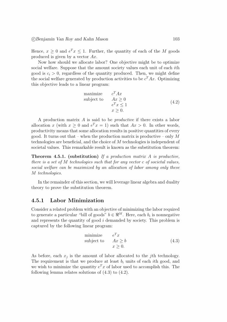
Now how should we allocate labor? One objective might be to optimizesocial welfare. Suppose that the amount society values each unit of each ithgood is ci > 0, regardless of the quantity produced. Then, we might definethe social welfare generated by production activities to be cT Ax. Optimizingthis objective leads to a linear program:

maximize cT Axsubject to Ax ≥ 0

eT x ≤ 1x ≥ 0.

(4.2)

A production matrix A is said to be productive if there exists a laborallocation x (with x ≥ 0 and eT x = 1) such that Ax > 0. In other words,productivity means that some allocation results in positive quantities of everygood. It turns out that – when the production matrix is productive – only Mtechnologies are beneficial, and the choice of M technologies is independent ofsocietal values. This remarkable result is known as the substitution theorem:

Theorem 4.5.1. (substitution) If a production matrix A is productive,there is a set of M technologies such that for any vector c of societal values,social welfare can be maximized by an allocation of labor among only theseM technologies.

In the remainder of this section, we will leverage linear algebra and dualitytheory to prove the substitution theorem.

4.5.1 Labor Minimization

Consider a related problem with an objective of minimizing the labor requiredto generate a particular “bill of goods” b ∈ <M . Here, each bi is nonnegativeand represents the quantity of good i demanded by society. This problem iscaptured by the following linear program:

minimize eT xsubject to Ax ≥ b

x ≥ 0.(4.3)

As before, each xj is the amount of labor allocated to the jth technology.The requirement is that we produce at least bi units of each ith good, andwe wish to minimize the quantity eT x of labor used to accomplish this. Thefollowing lemma relates solutions of (4.3) to (4.2).

104

Lemma 4.5.1. Let x∗ be an optimal solution to (4.2) and let b = Ax∗. Then,the set of optimal solutions to (4.3) is the same as the set of optimal solutionsto (4.2).

Proof: Note that eT x∗ = 1; if this were not true, x∗/eT x∗ would beanother feasible solution to (4.2) with objective value cT Ax∗/eT x∗ > cT x∗,which would contradict the fact that x∗ is an optimal solution.

We now show that x∗ (and therefore any optimal solution to (4.2)) is anoptimal solution to (4.3). Let x be an optimal solution to (4.3). Assume forcontradiction that x∗ is not an optimal solutoin to (4.3). Then, eT x < eT x∗

and

cT Ax/eT x = cT b/eT x > cT b/eT x∗ = cT Ax∗.

Since x/eT x is a feasible solution to (4.2), this implies that x∗ is not anoptimal solution to (4.2), which is a contradiction. The conclusion is that x∗

is an optimal solution to (4.3).

Since the fact that x∗ is an optimal solution to (4.3) implies that eT x =eT x∗ = 1. It follows that x is a feasible solutoin to (4.2). Since cT Ax ≥cT b = cT Ax∗, x is also an optimal solution to (4.2).

4.5.2 Productivity Implies Flexibility

Consider M technologies, each of which produces one of the M goods. To-gether they can be described by an M × M production matrix A. Inter-estingly, if A is productive then any bill of goods can be met exactly byappropriate application of these technologies. This represents a sort of flexi-bility – any demands for goods can be met without any excess supply. Thisfact is captured by the following lemma.

Lemma 4.5.2. If a square production matrix A ∈ <M×M is productive thenfor any b ≥ 0, the equation Ax = b has a unique solution x ∈ <M , whichsatisfies x ≥ 0.

Proof: Since A is productive, there exists a vector x ≥ 0 such thatAx > 0. The fact that only one element of each column of A is positiveimplies that x > 0.

Since the rows of A are linearly independent, Ax = b has a unique solutionx ∈ <N . Assume for contradiction that there is some b̂ ≥ 0 and x̂ with atleast one negative component such that Ax̂ = b̂. Let

α = min{α ≥ 0|αx + x̂ ≥ 0},


and note that α > 0 because some component of x̂ is negative. Since onlyone element of each column of A is positive, this implies that at least onecomponent of A(αx + x̂) is nonpositive.

Recall that Ax > 0 and Ax̂ ≥ 0, and therefore

Ax̂ < αAx + Ax̂ = A(αx + x̂),

contradicting the fact that at least one component of A(αx+x̂) is nonpositive.

4.5.3 Proof of the Substitution Theorem

Since A is productive, there exists a vector x ≥ 0 such that Ax > 0. Letb1 = Ax and consider the labor minimization problem:

minimize eT xsubject to Ax ≥ b1

x ≥ 0.

Let x1 be an optimal basic feasible solution and note that Ax1 ≥ b1 > 0.Since x1 is a basic feasible solution, at least N − M components must beequal to zero, and therefore, at most M components can be positive. Hence,the allocation x1 makes use of at most M technologies. Lemma 4.5.2 impliesthat these M technologies could be used to fill any bill of goods.

Given an arbitrary bill of goods b2 ≥ 0, we now know that there is a vectorx2 ≥ 0, with x2

jk= 0 for k = 1, . . . , N −M , such that Ax2 = b2. Note that

x2 ≥ 0 and satisfies N linearly independent constraints of and is therefore abasic feasible solution of the associated labor minimization problem:

minimize eT xsubject to Ax ≥ b2

x ≥ 0.

Let y1 be an optimal solution to the dual of the labor minimization problemwith bill of goods b1. By complementary slackness, we have (e−AT y1)T x1 =0. Since x2

j = 0 if x1j = 0, we also have (e − AT y1)T x2 = 0. Further,

since Ax2 = b2, we have (Ax2 − b2)T y1 = 0. Along with the fact that x2

is a feasible solution, this gives us the complementary slackness conditionsrequired to ensure that x2 and y1 are optimal primal and dual solutions tothe labor minimization problem with bill of goods b2.

We conclude that there is a set of M technologies that is sufficient toattain the optimum in the labor minimization problem for any bill of goods.It follows from Lemma 4.5.1 that the same set of M technologies is sufficientto attain the optimum in the social welfare maximization problem for anysocietal values.

106

4.6 Exercises

Question 1

Consider the following linear program (LP).

max x1 − x2

s.t. − 2x1 − 3x2 ≤ −4

−x1 + x2 ≤ −1

x1, x2 >= 0

(a) Plot the feasible region of the primal and show that the primal objec-tive value goes to infinity.

(b) Formulate the dual, plot the feasible region of the dual, and showthat it is empty.

Question 2

Convert the following optimization problem into a symmetric form linearprogram, and then find the dual.

max − x1 − 2x2 − x3

s.t. x1 + x2 + x3 = 1

|x1| ≤ 4

x1, x2, x3 ≥ 0

Note: |x| denotes the absolute value of x.

Question 3

consider the LP

max − x1 − x2

s.t. − x1 − 2x2 ≤ −3

−x1 + 2x2 ≤ 4

x1 + 7x2 ≤ 6

x1, x2 ≥ 0

(a) solve this problem in Excel using solver. After solver finds an optimalsolution, ask it to generate the sensitivity report.


(b) Find the dual of the above LP. Read the shadow prices from thesensitivity report, and verify that it satisfies the dual and gives the samedual objective value as the primal.

Question 4

Consider the LP

min 2x1 + x2

s.t. x1 + x2 ≤ 6

x1 + 3x2 ≥ 3

x1, x2, x3 ≥ 0

Note: there is an x3.(a) plot the feasible region and solve the problem graphically.(b) Rearrange into symmetric form and find the dual. Solve the dual graph-ically.(c) Verify that primal and dual optimal solutions satisfy the Strong DualityTheorem.

Question 5

(a) Consider the problem of feeding an army presented in Section 3.1.2. Pro-vide a dual linear program whose solution gives sensitivities of the cost ofan optimal diet to nutritional requirements. Check to see whether the sensi-tivities computed by solving this dual linear program match the sensitivitiesgiven by Solver when solving the primal.

(b) Suppose a pharmaceutical company wishes to win a contract with thearmy to sell digestible capsules containing pure nutrients. They sell threetypes of capsule, with 1 grams of carbohydrates, 1 gram of fiber, and 1grams of protein, respectively. The army requires that the company providea price for each capsule independently, and that substituting the nutritionalvalue of any food item with capsules should be no more expensive thanbuying the food item. Explain the relation between the situation faced bythe pharmaceutical company and the dual linear program.

108

Question 6

Consider a symmetric form primal linear program:


x ≥ 0.

(a) Find the dual of this problem. Noting that max f(x) = min−f(x)rearrange the dual into symmetric form. Take the dual of you answer, andrearrange again to get into symmetric form.

(b) Explain why the sensitivities of the optimal dual objective to the dualconstraints should be optimal primal variables.

Question 7

Recall Question 8, Homework 4, the diet Problem for the pigs. We found anoptimal solution for that problem (see Solution Homework 4). Now, supposethat Dwight doesn’t have a good estimate of the price of Feed type A becauseof some turbulence in the market. Therefore, he would like to know howsensitive is his original optimal solution with respect to changes in the priceof Feed Type A. In particular, in what range around $0.4 can the price ofFeed Type A change, without changing the original optimal solution? Forprices out of this range, what are the new optimal solutions? Now supposeDwight doesn’t have a good estimate of the requirements of vitamins. Inwhat range around 700 does the requirement of vitamins can change withoutchanging the original optimal solution? For values out of this range, whatare the new optimal solutions? Your arguments should be geometric (andnot based on Excel), that is, you should draw the problem in R2 and seewhat is going on.

Question 8

Consider the linear program

maximize −qT zsubject to Mz ≤ q

z ≥ 0.

where

M =

[0 A

−AT 0

], q =

[c−b

], z =

[xy

].


a) Derive the dualb) Show that the optimal solution to the dual is given by that of the primaland vice-versa.c) Show that the primal problem has an optimal solution if and only if it isfeasible.

Question 9

Consider the following LP.


x ≥ 0.

Show that if A, b and c are all positive, then both the primal and dualfeasible regions are non-empty.

Question 10

Why is it that, if the primal has unique optimal solution x∗, there is asufficiently small amount by which c can be altered without changing theoptimal solution?

Question 11 - Games and Duals

Show that the linear programs given in the notes to determine the strategiesof player 1 and player 2 are indeed duals of one another.

Question 12 - Drug Runners

Consider the drug running example from the notes. Imagine the drug lordhas a 4th alternative which involves transporting his drugs overland.

a) Suppose that the DEA can reassign its agents from coastguard dutyto guarding the border, and if it does so any shipment of drugs transportedoverland will be caught. Will the drug lord ever choose to send shipmentsoverland? If so, with what probability? If not, why not.

b) Suppose that guarding the border does not require the coastguard toreassign its agents, so that it can still guard a port (for instance, suppose thecustoms agents at the border are sufficiently equipped to detect most drugshipments). Suppose that an overland shipment will get through 85% of thetime. Will the drug lord ever choose to go overland? With what probability?

110

c) Suppose the percentage in part b) were changed to %80. What wouldbe the probability now.

d) Suppose the percentage in part b) were changed to %90. What wouldbe the probability now.

e) Suppose that if the DEA reassigns its agents to the border, they willcertainly catch any overland drug shipments, but if the agents are not reas-signed, then the customs agents will catch %80 of all drug shipments. Shouldthe DEA ever assign their agents to the border? With what probability?

Question 13 - Elementary Asset Pricing and Arbitrage

You are examining a market to see if you can find arbitrage opportunities.For the same of simplicity, imagine that there are M states that the marketcould be in next year, and you are only considering buying a portfolio now,and selling it in a years time. There are also N assets in the market, withprice vector ρ ∈ <N . The payoff matrix is P . So, the price of asset i is ρi

and the payoff of asset i in state j is Pji.You have observed some relationships amongst the prices of the assets,

in particular you have found that the price vector is in the row space of P .a) Suppose that ρT = qT P for some q ∈ <M . An elementary asset is

another name for an Arrow-Debreu security. That is, it is an asset that pays$1 in a particular state of the market, and $0 in any other state. So, thereare M elementary assets, and the ith elementary asset pays $1 if the marketis in state i, and $0 otherwise. Suppose that the ith elementary asset can beconstructed from a portfolio x ∈ <N . What is the price of x in terms of qand ρ? (Assume that there are no arbitrage opportunities.)

b) Suppose that however I write ρ as a linear combination of rows of P ,the coefficient of each row is non-negative. Is it possible for there to be anarbitrage opportunity? If not, why not. If so, give an example.

c) Suppose that ρ can be written as a linear combination of rows of P ,where the coefficient of each row is non-negative. Is it possible for their to bean arbitrage opportunity? If not, why not. If so, give an example. Note, thisis a weaker condition than (b) because there may be many ways of writing ρas a linear combination of rows of P .

Hint: Note that ρ being in the row space of P means that there is a vectorq such that ρT = qT P . Consider a portfolio x.

chapter 4 duality - stanford universityashishg/msande111/notes/chapter4.pdf · chapter 4 duality...

Documents