chapter 4 algorithm to solve job sequencing...
TRANSCRIPT

66
CHAPTER 4
ALGORITHM TO SOLVE JOB SEQUENCING PROBLEM
Job sequencing is the arrangement of the task that is to be performed or processed in a
machine in that particular order. Job sequencing problem has become the major problem
in the computer field. A finite set of n jobs where each job consists of a chain of
operations and a finite set of m machines where each machine can handle at most one
assignment at a time. Each assignment needs to be evaluated during an uninterrupted
period of a given length on a given machine and our Purpose is to find a inventory, that
is, an allocation of the operations to time intervals to machines that has minimal length.
Solving a problem or getting a job done by a computer can be quite a demanding task.
This is because it requires considerable thought, careful planning, and attention to details.
It can also be challenging and exciting with possibilities for creative satisfaction. This is
because when we are solving a problem with a computer, we are essentially teaching a
dumb servant how to do a job. We have already seen that the description of how to do
work is initially prepared in form of an algorithm and we did give a definition! But that
definition is to be used with some care. We should always remember the capabilities and
limitations of the executing representative, the computer. Components of any model can
be of
67
• Decision variables (What we can change to upgrade the system, i.e., model output)
• Parameters (Model input values, i.e., values that cannot be modified)
• Objective function (E.g. profit, quality to be maximized, costs, time to be minimized)
• Constraints (Determine which decision variable values are allowed)
Three basic types of decision variables are described as follows
• Sequence (Permutation of the jobs)
• Schedule (Allocation of the jobs in a more complex environment)
• Scheduling policy (Determines the next job, given the present state of the system)
Other variables are regarded as dynamic data, or as auxiliary variables. Some of the
auxiliary variables are specified as follows.
Completion time (Cij)
Lateness (Lj)
Tardiness (Tj)
Makespan (Mj)
There are three primary objectives (goals) which apply to all inventory problems. They
are
Job completions should not be “late” (about due dates).
The course of the time during which a job stays in the system should be
“minimum” (about flow time)

68
It is greedy to fully utilize the capacities of work centers (about work center
utilization).
A schedule is a job sequence determined for every machine of the processing system.
Scheduling is a decision-making process of allocating limited resources to activities over
time. The schedule can be characterized by starting or completion times of all operations
of the jobs. The objective is to construct a schedule that minimizes a given objective
function. The scheduling task is shown in figure 1.
Fig 1: Scheduling Task
Standard scheduling requirements are specified as follows.
A job cannot be processed by two or more machines at a time,
A machine cannot process two or more jobs at the same time.

69
Depending on the type of scheduling system, specific constraints should be satisfied (jobs
may be released at different times, there may be allowed preemption of jobs by other
jobs, etc.).The various scheduling issues are described as follows
Scheduling accord with the timing of operations
The assignment is the allocation and prioritization of demand
Significant issues are the type of scheduling, backword or forward
The criteria for priorities
There are two types of scheduling. They are
Forward scheduling
Backward scheduling
Forward scheduling starts as soon as the requirements are known. It produces a feasible
schedule though it may not meet due dates. It frequently results in buildup of work in
process inventory.
Fig 2: Types of scheduling

70
Backward scheduling begins with the due date and schedules the final operation first.
Schedule is produced by working conversely though the processes Resources may not be
available to accomplish the schedule. The forward and the backward scheduling is shown
in the figure 2.
In a typical job scheduling conditions, there is a centralized scheduling stage with a set of
on-demand technologies to support its functions. The IT operations and significance
scheduling teams interact with the scheduler through a client tier or a Web interface.
Conventionally, job scheduling solutions performed their work using platform specific
promotors, including Microsoft Windows, UNIX, Linux, and mainframe operating
systems. Job scheduling solutions schedule, define and manage application jobs, which
are the individual steps needed to deliver the services. There has also been an effort to
integrate and schedule jobs using the latest business intelligence, data warehouse,
transform, and extract, load (ETL) applications. These solutions require integration of
database activities.
The solutions process data from multiple applications across the enterprise to deliver the
business insight required to make the right strategic decisions at the right time.
Administering dependency logic and automating job step sequencing are critical to the
delivery of relevant and timely information for strategic decision making. Job scheduling
solutions can also manage backup, file delivery, and storage processes. More recently,
job schedulers have been integrated with virtualization solutions and certain cloud
services that have the capability to schedule jobs in a virtualized environment.

71
Fig 3: Types of scheduling problems
There are two fundamental kinds of scheduling problems. They are given as follows
Static scheduling problem
Dynamic scheduling problem
The static scheduling problem deals with the problem which consists of a fixed set of
jobs which are to be all completed. In this static scheduling the number of jobs does not
change. The Dynamic scheduling problem deals with scheduling of a continuous
situation, which means that, new jobs are continually added to the production
environment. The types of scheduling problems are shown in figure 3.
The static scheduling problem contains a fixed set of jobs which are to be completed. The
typical basic assumptions in this kind of problem can be stated as follows;

72
Complete set of jobs arrive simultaneously, and all respective work centers are
available at that time.
Majority of the static scheduling problems use a criterion called “minimum make span ”
which can be defined as the minimum total time to process all subject jobs. This standard
is related with the scheduling objective which is about “flow time”.
Fig 4: Static scheduling approach
The static scheduling approach makes use of deterministic solutions and stochastic
solutions. The deterministic solutions use known and non varying process times and it
uses methods producing optimum results and methods utilizing heuristic procedures. The

73
static scheduling approach is shown in the figure 4. Methods producing Optimum results
are only applicable to relatively small problems. Methods utilizing heuristic procedures
are also called as dispatching or sequencing rules by which scheduling decisions are
made sequentially. Stochastic solutions use process times which are subject to random
variations. The dynamic scheduling approach is shown in figure 5.
Fig 5: Dynamic scheduling approach
Analytical approaches like deterministic solutions, stochastic solutions had been
developed which are “based on queuing models that provide expected steady state
conditions for certain kinds of situations and time distributions. Typically, the criteria
used in such queuing cases are; Average Flow Time, Average Work-in-process or
number of jobs in the system and Work/machine center utilization. To find a solution to
dynamic scheduling problems, usually the approach is, to use different “dispatching
rules” at the work centers.
74
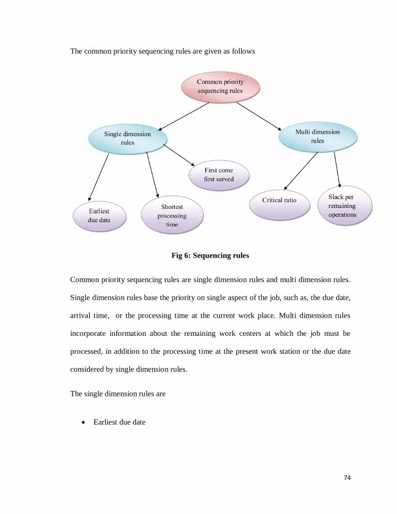
The common priority sequencing rules are given as follows
Fig 6: Sequencing rules
Common priority sequencing rules are single dimension rules and multi dimension rules.
Single dimension rules base the priority on single aspect of the job, such as, the due date,
arrival time, or the processing time at the current work place. Multi dimension rules
incorporate information about the remaining work centers at which the job must be
processed, in addition to the processing time at the present work station or the due date
considered by single dimension rules.
The single dimension rules are
Earliest due date

75
There may be different ways to set the due dates of jobs. For example, a due date might
have been calculated by computerized methods as in MRP or might have been simply
determined by the customer.
The job with the earliest due date is the job which is to be scheduled next.
Shortest processing time
It is the king of the priority sequencing rules. The job which has the shortest processing
time is scheduled next.
First come first served
The job which arrives the work station earlier than the others has the highest priority and
is to be scheduled next.
The Multi dimension rules are
Critical ratio
The critical ratio is calculated by dividing “the time remaining until the due date of the
job” by the “remaining total shop time for the job”.
Slack per remaining operations
Slack is the difference between “the time remaining until the due date of the job” and
“remaining total shop time for the job” including that of the operation being scheduled.
The job’s priority is determined by dividing the slack by the number of the operations
that remain including the operation which is being scheduled.

76
Scheduling deals with the problems of optimal arrangement, sequencing and timetabling.
Sequencing is similar to that of scheduling. Job Sequencing is the arrangement of the
tasks required to be carried out sequentially. The job sequencing problem can be solved
by means of the new modified heuristic technique called time deviation method. The
modified time deviation method can be used for processing n jobs through two machines,
n jobs through three machines, n jobs through m machines.
4.1 MODIFIED TIME DEVIATION METHOD
Time deviation method is used to obtain the optimal sequence of the jobs. In this method
time duration table is calculated for each job in the row wise and the column wise.
Maximum time duration of the row minus the time duration of the cell gives the
row deviation of the cell in the time duration table.
ijiij trp (1)
Where ir is the maximum time of the
thi row, ijp is the row time deviation of the
thji ),( cell and ijt be the time required for processing thi
job on the thj
machine.
Maximum time duration of the column minus the time duration of the cell gives
the column deviation of the cell in the time duration table.
ijiij tsc (2)
Where is
is the maximum time of the
thi column, ijc is the column time deviation of
the thji ),(
cell and ijt be the time required for processing
thi job on thethj
machine.
77
The time deviation method used for solving job sequencing problem is explained with the
examples.
4.2 SEQUENCING N JOBS IN TWO MACHINES
The N jobs can be sequenced in two machines by the following steps.
Calculate the time deviation table for the sequencing problem.
The cell which has both the time deviation vectors as zero for machine 1, perform
that job first.
If more than one cell has both vectors as zero then calculate sum deviation of the
corresponding columns. Cell which has largest sum deviation is performed first
and so on.
Similar steps are followed for machine 2 but here the jobs are performed lastly.
Again calculate the reduced time deviation table for all non assigned jobs and
continue the steps mentioned above.
Stop the process if we get sequence involving all jobs.
Arrange the obtained sequence in reverse order to get minimum total elapsed
time.
Sequencing N jobs in two machines can be explained by the following example.
Example: Processing of N jobs in two machines is given as follows

78
Jobs/Machines J1 J2 J3 J4 J5 J6 J7 J8 J9
M1 2 5 4 9 6 8 7 5 4
M2 6 8 7 4 3 9 3 8 11
The time deviation table will be first calculated for the given problem according to the
equations (1) and (2). The table is as follows
Jobs/Machines J1 J2 J3 J4 J5 J6 J7 J8 J9
M1 (7,4) (4,3) (5,3) (0,0) (3,0) (1,1) (2,0) (4,3) (5,7)
M2 (5,0) (3,0) (4,0) (7,5) (8,3) (2,0) (8,4) (3,0) (0,0)
The jobs J4 of machine 1 and J9 of machine 2 has both vectors zero and is assigned as
follows
J4 J9
The reduced time duration table for the remaining jobs is as follows
Jobs/Machines J1 J2 J3 J5 J6 J7 J8
M1 2 5 4 6 8 7 5
M2 6 8 7 3 9 3 8

79
The time deviation table is calculated for this sequence as follows
Jobs/Machines J1 J2 J3 J5 J6 J7 J8
M1 (6,4) (3,3) (4,3) (2,0) (0,1) (1,0) (3,3)
M2 (3,0) (1,0) (2,0) (6,3) (0,0) (6,4) (1,0)
Job J6 in machine 2 has both the vectors as zero and so it is assigned to the sequence as
J4 J6 J9
The time duration table for the jobs J1, J2, J3, J5, J7, and J8 is specified and the jobs J4,
J6, J9 will not be specified in this table since it is assigned to the machines as shown
above.
Jobs/Machines J1 J2 J3 J5 J7 J8
M1 2 5 4 6 7 5
M2 6 8 7 3 3 8
The time deviation table for the above jobs is calculated as follows

80
Jobs/Machines J1 J2 J3 J5 J7 J8
M1 (5,4) (2,3) (3,3) (1,0) (0,0) (2,3)
M2 (2,0) (0,0) (1,0) (5,3) (5,4) (0,0)
The jobs J7 in machine 1, J2 and J8 in machine 2 have both vectors zero and it is
assigned as follows
J4 J7 J2 J8 J6 J9
The time duration table for the remaining jobs J1, J3, J5 is given as follows
Jobs/Machines J1 J3 J5
M1 2 4 6
M2 6 7 3
The time deviation table for the above jobs is calculated as follows
Jobs/Machines J1 J3 J5
M1 (4,4) (2,3) (0,0)
M2 (1,0) (0,0) (4,3)
Here J5 in machine 1 and J3 in machine 2 contain both the vectors as zero and so it is
assigned and the remaining J1 is also assigned as follows

81
J4 J7 J5 J1 J3 J2 J8 J6 J9
This sequence is then arranged in the reverse order from last obtained job to the machine
1 jobs and machine 2 jobs. It is represented as follows
J1 J5 J7 J4 J9 J6 J8 J2 J3
The above sequence is the required sequence for the given problem. The minimum total
elapsed time is calculated for this job sequence. The total elapsed time is given as Total
Elapsed Time = Time between starting the first job in the optimum sequence on machine
1 and completing the last job in the optimum sequence on machine M.
Job sequence Machine 1
Time-in Time-out
Machine 2
Time-in Time-out
1
5
7
4
9
6
8
2
3
0
2
8
15
24
28
36
41
46
2
8
15
24
28
36
41
46
50
2
8
11
14
18
29
38
46
54
8
11
14
18
29
38
46
54
61
The minimum total elapsed time thus obtained is 61 hours.

82
4.3 SEQUENCING N JOBS IN THREE MACHINES
The N jobs can be sequenced in three machines by the following steps
Calculate the time deviation table for the sequencing problem.
The cell which has both the time deviation vectors as zero for machine 1, perform
that job first. If both the time deviation vectors are zero in machine 3 then perform
that job in the last and if the vectors are zero in machine 2 then find the sum of
deviation vectors separately for above and below of the zero cell. Compare both
the deviations.
Perform that particular job first if the sum of deviation vectors above the cell is
less than the other one. If both are same then perform the job either in first or last.
Again calculate the reduced time deviation table for all non assigned jobs and
continue the steps mentioned above.
Stop the process if we get sequence involving all jobs.
Arrange the obtained sequence in reverse order to get minimum total elapsed
time.
Example: N jobs to be processed in three machines are given as follows
Jobs/Machines J1 J2 J3 J4 J5 J6 J7
M1 3 8 7 4 9 8 7
M2 4 3 2 5 1 4 3
M3 6 7 5 11 5 6 12

83
The time deviation table will be first calculated for the given problem according to the
equations (1) and (2). The table is as follows
Jobs/Machines J1 J2 J3 J4 J5 J6 J7
M1 (6, 3) (1, 0) (2, 0) (5, 7) 0, 0) (1, 0) (2, 5)
M2 (1, 2) (2, 5) (3, 5) (0, 6) (4, 8) (1, 4) (2, 9)
M3 (6, 0) (5, 1) (7, 2) (1, 0) (7, 4) (6, 2) (0, 0)
Jobs J5 in machine 1 and J7 in machine 3 have both the vectors zero and so they are
assigned to job sequence as follows
J5 J7
The time duration table for the jobs other than J5 and J7 are given as follows
Jobs/Machines J1 J2 J3 J4 J6
M1 3 8 7 4 8
M2 4 3 2 5 4
M3 6 7 5 11 6
The time deviation table for the above jobs is specified as follows
Jobs/Machines J1 J2 J3 J4 J6
M1 (5, 3) (0, 0) (1, 0) (4, 7) (0, 0)
M2 (1, 2) (2, 4) (3, 5) (0, 6) (1, 4)
M3 (5, 0) (4, 1) (6, 2) (0, 0) (5, 2)

84
The jobs J2, J6 in machine 1 and J4 in machine 3 have both the vectors zero and so they
are arranged as follows
J5 J6 J2 J4 J7
The time duration table for the remaining jobs is given as follows
Jobs/Machines J1 J3
M1 3 7
M2 4 2
M3 6 5
The time deviation table for the above two jobs are given as follows
Jobs/Machines J1 J3
M1 (4, 3) (0, 0)
M2 (0, 2) (2, 5)
M3 (0, 0) (1, 2)
The job J3 in machine 1 and the job J1 in machine 3 are then assigned to the sequence as
follows
85
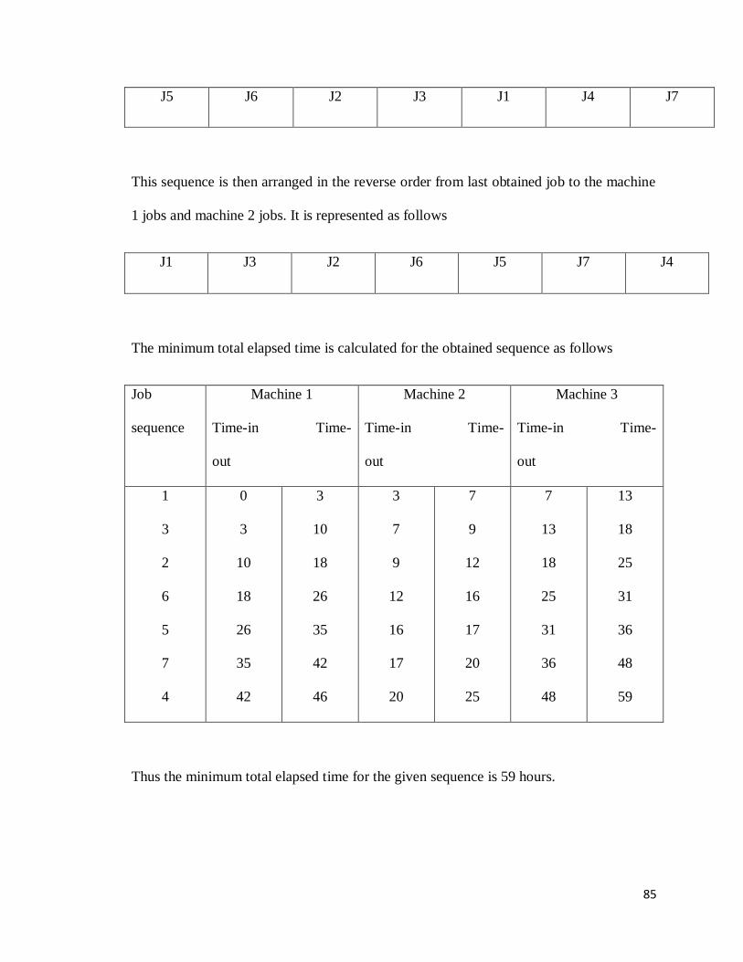
J5 J6 J2 J3 J1 J4 J7
This sequence is then arranged in the reverse order from last obtained job to the machine
1 jobs and machine 2 jobs. It is represented as follows
J1 J3 J2 J6 J5 J7 J4
The minimum total elapsed time is calculated for the obtained sequence as follows
Job
sequence
Machine 1
Time-in Time-
out
Machine 2
Time-in Time-
out
Machine 3
Time-in Time-
out
1
3
2
6
5
7
4
0
3
10
18
26
35
42
3
10
18
26
35
42
46
3
7
9
12
16
17
20
7
9
12
16
17
20
25
7
13
18
25
31
36
48
13
18
25
31
36
48
59
Thus the minimum total elapsed time for the given sequence is 59 hours.
86
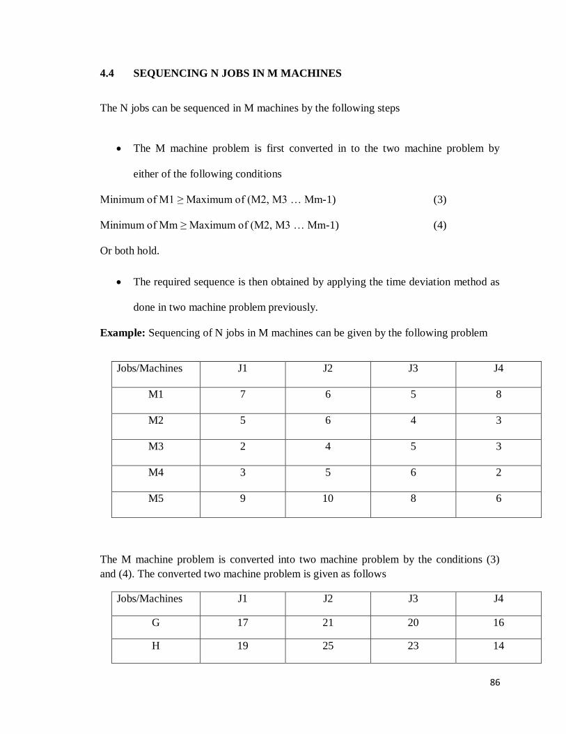
4.4 SEQUENCING N JOBS IN M MACHINES
The N jobs can be sequenced in M machines by the following steps
The M machine problem is first converted in to the two machine problem by
either of the following conditions
Minimum of M1 ≥ Maximum of (M2, M3 … Mm-1) (3)
Minimum of Mm ≥ Maximum of (M2, M3 … Mm-1) (4)
Or both hold.
The required sequence is then obtained by applying the time deviation method as
done in two machine problem previously.
Example: Sequencing of N jobs in M machines can be given by the following problem
Jobs/Machines J1 J2 J3 J4
M1 7 6 5 8
M2 5 6 4 3
M3 2 4 5 3
M4 3 5 6 2
M5 9 10 8 6
The M machine problem is converted into two machine problem by the conditions (3)
and (4). The converted two machine problem is given as follows
Jobs/Machines J1 J2 J3 J4
G 17 21 20 16
H 19 25 23 14
87
The required job sequence is then obtained by the procedure that is normally applied for
the two machine problem as explained by the above example.
4.5 Conclusion
Thus the new modified heuristic technique called time deviation method is used to obtain
the required job sequence and the minimum total elapsed time is also calculated for this
sequence of jobs by the usual procedure as specified in the above examples. Processing
of N jobs in 2 machines, Processing of N jobs in 3 machines, Processing of N jobs in M
machines were also explained by the examples.