chapter 3.smai.emath.fr › cemracs › cemracs03 › boltzmann.pdf · (summary) pierre degond -...

(Summary) (Conclusion)Pierre Degond - overview of kinetic models - Luminy, July 2003

1

Chapter 3.

Theory of the Boltzmann equation

P. Degond

MIP, CNRS and Université Paul Sabatier,

118 route de Narbonne, 31062 Toulouse cedex, France

[email protected] (see http://mip.ups-tlse.fr)


2Summary

1. Properties of the Boltzmann collision operator

2. Overview of existence results

3. Variants of the Boltzmann equation

4. Summary and conclusion


3

1. Properties of the Boltzmann collisionoperator


4The Boltzmann equation

∂f

∂t+ v · ∇xf = Q(f)

Q(f) =

∫

v1∈R3

∫

~n∈S2+

σ(|v − v1|, cosθ) |v − v1|

[f(v′)f(v′1) − f(v)f(v1)] dv1 d~n

v′ = v − (v − v1, ~n)~n , v′1 = v1 + (v − v1, ~n)~n

cos θ =|(v − v1, ~n)|

|v − v1|


5Microreversibility

à ~n fixed in S2+:

(v, v1)J

−→ (v′, v′1) involution

J2 = Id , J = J−1 , det J = 1

à

σ(v, v1) = σ(v′, v′1)

Microreversibility: Probability of the directcollision is the same as the inverse one


6Weak form

à Let ψ be any ”regular” test function

à Denote f ′ = f(v′), f ′1 = f(v′1), etc, V1 = v − v1.

∫

Q(f)ψdv =

= −1

2

∫

(f ′ f ′1 − f f1)(ψ′ − ψ)σ|V1|d~n dv dv1 =

−1

4

∫

(f ′ f ′1 − f f1)(ψ′ + ψ′

1 − ψ − ψ1)σ|V1|d~n dv dv1

=1

2

∫

f f1(ψ′ + ψ′

1 − ψ − ψ1)σ|V1|d~n dv dv1


7Collisional invariant

à ψ collisional invariant ⇐⇒∫

Q(f)ψdv = 0 , ∀f

à ⇐⇒ ψ satisfies

ψ(v′) + ψ(v′1) − ψ(v) − ψ(v1)

∀(v, v1, v′, v′1) s.t. ∃~n and (v′, v′1) = J(v, v1)

à ⇐⇒ ∃A,C ∈ R, B ∈ R3 s.t.

ψ(v) = A+B · v + C|v|2


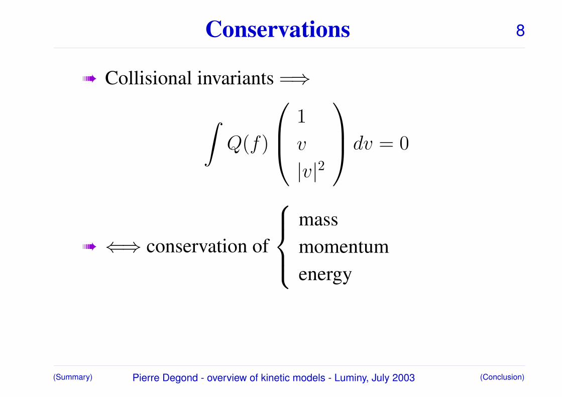
8Conservations

à Collisional invariants =⇒

∫

Q(f)

1

v

|v|2

dv = 0

à ⇐⇒ conservation of

massmomentumenergy


9Conservations (cont)

∂f

∂t= Q(f) =⇒

∂f

∂t

∫

f

1

v

|v|2

dv = 0


10H-theorem

à Take ψ = ln f in the weak formulation

à Use that ln is an increasing function

∫

Q(f) ln fdv =

−1

4

∫

(f ′ f ′1 − f f1)(ln f′ + ln f ′1 − ln f − ln f1)

σ|V1|d~n dv dv1

= −1

4

∫

(f ′ f ′1 − f f1)(ln f′f ′1 − ln ff1)σ|V1|d~n dv dv1

≤ 0


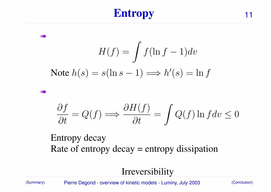
11Entropy

à

H(f) =

∫

f(ln f − 1)dv

Note h(s) = s(ln s− 1) =⇒ h′(s) = ln f

à

∂f

∂t= Q(f) =⇒

∂H(f)

∂t=

∫

Q(f) ln fdv ≤ 0

Entropy decayRate of entropy decay = entropy dissipation

Irreversibility


12Equilibria

Q(f) = 0 =⇒

∫

Q(f) ln fdv = 0

⇐⇒

∫

(f ′ f ′1 − f f1)(ln f′f ′1 − ln ff1)

σ|V1|d~n dv dv1 = 0

⇐⇒ ln f is a collisional invariant⇐⇒ ∃A,C ∈ R+, B ∈ R

3s.t.f = exp(A+B · v + C|v|2)

à Maxwellian distribution


13Maxwellian

à Other expression:

Mn,u,T =n

(2πT )3/2exp

(

−|v − u|2

2T

)

(n, u, T ) straightforwardly related w. (A,B,C)

∫

Mn,u,T

1

v

|v|2

dv =

n

nu

n|u|2 + 3nT


14Characterization of Maxwellians

à (i) Entropy dissipation∫

Q(f) ln fdv ≤ 0 and ≡ 0iff f = Maxwellian

à (ii) Entropy minimization subject to momentconstraints: let n, T ∈ R+, u ∈ R

3 fixed.

min{H(f) =

∫

f(ln f − 1)dv s.t.

∫

f

1

v

|v|2

dv =

n

nu

n|u|2 + 3nT

}

is realized by f = Mn,u,T .


15

2. Overview of existence results


16Homogeneous equation

à∂f

∂t= Q(f)

à Existence and uniqueness of classical solutions[Carleman], [Arkeryd], ...

à Convergence to a Maxwellian as t→ ∞[Desvillettes], [Wennberg], ...


17Non-homogeneous equation

à∂f

∂t+ v · ∇xf = Q(f)

à Difficulty: Q(f) quadratic in f

à ref. [DiPerna, Lions]: renormalized solutions i.e.satisfying:

(∂

∂t+ v · ∇x)β(f) = β ′(f)Q(f) in D′

∀β Lipschitz, s.t. |β ′(f)| ≤ C/(1 + f)

à Note: β ′(f)Q(f) grows linearly with f


18Perturbation of equilibria

à ref: [Ukai], [Nishida, Imai], ...

à M global Maxwellian (parameters (n, u, T ) areconstant indep. of x, t

à f = M + g, with ”g �M”

à Decompose

Q(f) = LMg + Γ(g, g)

à Prove operator v · ∇xg − LMg dissipative

à Compensates blow-up of Γ(g, g) if g small


19

3. Variants of the Boltzmann equation


20BGK operator

Q(f) = −ν(f −Mf)

where Mf = Mn,u,T is the Maxwellian with the samemoments as f i.e. (n, u, T ) are such that

∫

(Mf − f)

1

v

|v|2

dv = 0

i.e.

n

nu

n|u|2 + 3nT

=

∫

f

1

v

|v|2

dv


21Properties of BGK operator

à Shows the same ’algebraic’ properties as theBoltzmann operator

à (i) Collisional invariants:∫

Q(f)ψdv = 0, ∀f ⇐⇒ ψ(v) = A+B·v+C|v|2

à (ii) Equilibria:

Q(f) = 0 ⇐⇒ f = Mn,u,T


22Properties of BGK operator (cont)

à H-theorem∫

Q(f) ln fdv ≤ 0 (= 0 ⇐⇒ f = Mn,u,T )

à Simpler operatorß Theory simplerß Numerical simulations are easierß Some unphysical features (Prandtl number)


23Some references for BGK

à Existence of weak solutions [Perthame, Pulvirenti]

à Numerical solutions [Dubroca, Mieussens]

à Generalized BGK models [Bouchut, Berthelin]


24Landau operator

à grazing collision limit [Desvillettes]

à (i) Suppose ∃ parameter η s.t.

ση(|v − v1|, cos θ) ” −→ ” σ̄(|v − v1|)δ(θ − π/2)

à =⇒ QB(f) → QL(f)

QL(f) = ∇v ·

∫

σ̄(|v − v1|)S(v − v1)

(f1∇vf − f(∇vf)1) dv1

S(v) = Id −vv

|v|2


25Coulomb case

à ref. [D., Lucquin]

QηB(f) =

∫ ∫

|θ−π/2|>η

σC(|v − v1|, cosθ) |v − v1|

[f(v′)f(v′1) − f(v)f(v1)] dv1 d~n

with σC Coulomb scattering cross section. Note, Q0B

not defined because integral diverges

QηB(f)

η→0∼ | ln η|QL(f) +O(η)

ln η: Coulomb logarithm


26Theory of Landau equation

à Existence theory for Landau equation far frombeing as complete as for the Boltzmann equation

à Weak solutions for homogeneous equation[Arseneev]

à Linearized Landau equation [D., Lemou]

à Nonlinear Landau: Considerable amount of workrecently by [Alexandre, Desvillettes, Villani, ...]


27Other variants of Boltzmann

à Enskog eq. Keep the diameter of the spheres δfinite −→ space delocalization of the operator.ß Note: a result of convergence of a stochastic

particle system to the Enskog eq. by[Rezhakanlou]

à Quantum Boltzmann eq.:ff1 −→ ff1(1 ± f ′)(1 ± f ′1)

ß − sign: Pauli operator [Golse & Poupaud],[Dolbeault]

ß + sign: Bose-Einstein operator [Mischler et al]


28Variants (cont)

à Boltzmann for molecules with internal degrees offreedom −→ ”real gases” (as opposed to ”perfectgases”ß ref. [Neunzert, Strückmeier et al], [Le Tallec,

Perthame et al], . . .


29

4. Summary and conclusion


30Summary

à Properties of the Boltzmann operatorß Conservation (collisional invariants)ß Equilibria (Maxwellians)ß Relaxation (entropy decay)

à Existence theoryß Classical theory (perturbation of equilibria)ß Renormalized solutions [DiPerna, Lions]

à Variants of Boltzmannß Model BGK operatorß Grazing limit and the Landau operator


31Equilibria and Hydrodynamic limits

à Properties of the Boltzmann operator −→derivation of hydrodynamic equations

à Use of BGK operator −→ simpler theory

chapter 3.smai.emath.fr › cemracs › cemracs03 › boltzmann.pdf · (summary) pierre degond -...

Documents