chapter 3 simple lie algebras. classiﬁcation and representations. roots...

Chapter 3

Simple Lie algebras. Classification and

representations. Roots and weights

3.1 Cartan subalgebra. Roots. Canonical form of the

algebra

We consider a semi-simple (i.e. with no abelian ideal) Lie algebra. We want to construct a

canonical form of commutation relations modeled on the case of SU(2)

[Jz, J±] = ±J± [J+, J!] = 2Jz . (3-1)

It will be important to consider the algebra over C, at the price of “complexifying” it if it was

originally real. The adjoint representation will be used. As it is a faithful representation for a

semi-simple algebra, (i.e. ad X = 0 ! X = 0, see exercise B of Chap. 2), no information is

lost.

It may also be useful to remember that the complex algebra has a real compact version, in

which the real structure constants lead to a negative definite Killing form, and, as the repre-

sentations can be taken unitary, the elements of the Lie algebra (the infinitesimal generators)

may be taken as Hermitian (or antiHermitian, depending on our conventions).

3.1.1 Cartan subalgebra

We define first the notion of Cartan subalgebra. This is a maximal abelian subalgebra of g such

that all its elements are diagonalisable (hence simultaneously diagonalisable) in the adjoint

representation. That such an algebra exists is non trivial and must be established, but we shall

admit it.If we choose to work with the unitary form of the adjoint representation, the elements of g are Hermi-

tian matrices, and assuming that the elements of h are commuting among themselves ensures that they aresimultaneously diagonalizable.

This Cartan subalgebra is non unique, but one may prove that two distinct choices arerelated by an automorphism of the algebra g.

71

72 CHAPTER 3. CLASSIFICATION OF SIMPLE ALGEBRAS. ROOTS AND WEIGHTS.

For instance if g is the Lie algebra of a Lie group G and if h is a Cartan subalgebra of g, any conjugate ghg!1

of h by an arbitrary element of G is another Cartan subalgebra.

Let h be a Cartan subalgebra, call ! its dimension, it is independent of the choice of h and

it is called the rank of g. For su(2), this rank is 1, (the choice of Jz for example); for su(n), the

rank is n" 1. Indeed for su(n), a Cartan algebra is generated 1 by diagonal traceless matrices,

a basis of which is given by the n" 1 matrices

H1 = diag (1,"1, 0, · · · , 0), H2 = diag (0, 1,"1, 0, · · · , 0), · · · , Hn!1 = diag (0, · · · , 0, 1,"1) .

(3-2)

An arbitrary matrix of the Lie algebra, (in that representation), (anti-)Hermitian and trace-

less, is diagonalisable by a unitary transformation; its diagonal form is traceless and is thus

expressed as a linear combination of the hj; the original matrix is thus conjugate by a unitary

transformation of a linear combination of the hj. This is a general property, and one proves

(Cartan, see [Bu], chap. 16) that

If g is the Lie algebra of a group G, any element of g is conjugate by G of an element of h.

Application. Canonical form of antisymmetric matrices. Using the previous statement, prove theProposition If A = A" = "AT is a real skew-symmetric matrix of dimension N , one may find a real

orthogonal matrix O such that A = ODOT where D = diag (

!0 µj

"µj 0

"

j=1,··· ,n

) if N = 2n and D =

diag (0,

!0 µj

"µj 0

"

j=1,··· ,n

) if N = 2n + 1, with real µj .

If one allows the complexification of orthogonal matrices, one may fully diagonalise the matrix A in the form

D = diag (

!iµj 00 "iµj

"

j=1,··· ,n

) or D = diag (0,

!iµj 00 "iµj

"

j=1,··· ,n

). For a proof making only use of matrix

theory, see for example [M.L. Mehta, Elements of Matrix Theory, p 41].

3.1.2 Canonical basis of the Lie algebra

Let Hi, i = 1, · · · , ! be a basis of h. It is convenient to choose the Hi Hermitian. By definition

[Hi, Hj] = 0, (abelian subalgebra) or more precisely, since we are in the adjoint representation,

[ad Hi, ad Hj] = 0 . (3-3)

We may thus diagonalise simultaneously these adHi. We already know (some?) eigenvectors

of vanishing eigenvalue since #i, j, ad Hi Hj = 0, and we may complete them to make a basis

by finding a set of eigenvectors E! linearly independent of the Hj

ad Hi E! = "(i)E! (3-4)

i.e. a set of elements of g such that

[Hi, E!] = "(i)E! , (3-5)

1We use momentarily the “representation of definition” (made of n $ n matrices) rather than the adjointrepresentation.

3.1. CARTAN SUBALGEBRA. ROOTS. CANONICAL FORM OF THE ALGEBRA 73

with the "(i) not all vanishing (otherwise the subalgebra h would not be maximal).

The space h". In these expressions, the "(i) are eigenvalues of the operators adHi. Since

we chose Hermitian adHi, their eigenvalues "(i) are real. By linearity, for an arbitrary element

of h written as H =#

i hiHi,

ad (H)E! = "(H)E! , (3-6)

and the eigenvalue of ad (H) on E! is "(H) :=#

i hi"(i), which is a linear form on h. In general

linear forms on a vector space E form a vector space E", called the dual space of E. One may

thus consider the root ", of components "(i), as a vector of the dual space of h, hence " % h",

the root space. Note that "(Hi) = "(i).

Roots enjoy the following properties (&)

1. if " is a root, "" in another root;

2. the eigenspace of the eigenvalue " is of dimension 1 (no multiplicity);

3. if " is a root, the only roots of the form #" are ±";

4. roots " generate all the dual space h".

For proofs of 1., 2., 3., see below, for 4. see exercise A.

Number of roots. Since the Hj are diagonalisable, the total number of their eigenvectors

E! and Hi must be equal to the dimension of the space, here the dimension d of the adjoint

representation, i.e. of the Lie algebra g. As any (non vanishing by definition) root comes along

with its opposite, the number of roots " is even and equal to d " ! (with ! = rank(g)). We

denote ! the set of roots.

In the basis {Hi, E!} of g, the Killing form takes a simple form

(Hi, E!) = 0 (E!, E") = 0 unless " + $ = 0 . (3-7)

To show that, we write (H, [H #, E!]) = !(H #)(H,E!), and also, using the definition of the Killing form and thecyclicity of the trace

(H, [H #, E!]) = tr (adH[adH #, adE!]) = tr ([adH, adH #] adE!) = 0 (3-8)

since [ad H, adH #] = 0. It follows that #H,H # % h, !(H #)(H,E!) = 0, hence that (H,E!) = 0. Likewise

([H,E!], E") = !(H)(E!, E") = "(E!, [H,E" ]) = ""(H)(E!, E") (3-9)

again by the cyclicity of the trace, and thus (E!, E") = 0 if 'H : (! + ")(H) (= 0, i.e. if ! + " (= 0. Notethat the point 1. in (&) above follows simply from (3-7): if "! were not a root, E! would be orthogonal to allelements of the basis hence to any element of g, and the form would be degenerate, contrary to the hypothesisof semi-simplicity (and Cartan’s criterion). For an elegant proof of points 2. et 3. of (&), see [OR, p. 29].

The restriction of this form to the Cartan subalgebra is non-degenerate, since otherwise one

would have 'H % h, #H # % h : (H, H #) = 0, but (H,E!) = 0, thus #X % g, (H,X) = 0 and the

form would be degenerate, contrary to the hypothesis of semi-simplicity (and Cartan’s criterion,

Chap. 1, §4.4). The Killing form being non-degenerate on h, it induces an isomorphism between

h and h": to " % h" one associates the unique H! % h such that

#H % h "(H) = (H!, H) . (3-10)


(Or said di"erently, one solves the linear system gijhj! = "(i) which is of Cramer type since

gij = (Hi, Hj) is invertible.) One has also a bilinear form on h" inherited from the Killing form

)", $ * = (H!, H") , (3-11)

which we are going to use in § 2 to study the geometry of the root system.

It remains to find the commutation relations of the E! among themselves. Using the Jacobi

identity, one finds that

ad Hi[E!, E"] = [Hi, [E!, E"]] = [E!, [Hi, E"]" [E", [Hi, E!]] = (" + $)(i)[E!, E"] . (3-12)

Invoking the trivial multiplicity (=1) of roots, one sees that three cases may occur. If " + $

is a root, [E!, E"] is proportional to E!+", with a proportionality coe#cient N!" which will

be shown below to be non zero (see § 2.1 and exercise B). If " + $ (= 0 is not a root, [E!, E"]

must vanish. Finally if " + $ = 0 , [E!, E!!] is an eigenvector of all adHi with a vanishing

eigenvalue, thus [E!, E!!] = H % h. To determine that H, let us proceed like in (3-9)

(Hi, [E!, E!!]) = tr (ad Hi [ad E!, ad E!!]) = tr ([ad Hi, ad E!] ad E!!)

= "(i)(E!, E!!) = (Hi, H!)(E!, E!!) (3-13)

hence

[E!, E!!] = (E!, E!!)H! . (3-14)

To recapitulate, we have constructed a canonical basis of the algebra g

[Hi, Hj] = 0

[Hi, E!] = "(i)E!

[E!, E"] =

$%%%&

%%%'

N!"E!+" if " + $ is a root

(E!, E!!) H! if " + $ = 0

0 otherwise

(3-15)

Up to that point, the normalisation of the vectors Hi and E! has not been fixed. It is

common to choose, in accord with (3-7)

(Hi, Hj) = %ij (E!, E") = %!+",0 . (3-15)

(Indeed, the restriction of the Killing form to h, after multiplication by i to make the adHi

Hermitian, is positive definite.) With that normalisation, H! defined above by (3-10) satisfies

also

H! = ".H := "(i)Hi . (3-16)

3.2. GEOMETRY OF ROOT SYSTEMS 75

Note that E!, E!! and H! form an su(2) subalgebra

[H!, E±!] = ± )", " *E±! [E!, E!!] = H! . (3-17)

(This is in fact H!/)", " * that we identify with Jz, and that observation will be used soon.)

Any semi-simple algebra thus contains an su(2) algebra associated to each of its roots.

Note that with the normalisations of (3-15), the Killing metric reads in the basis {Hi, E!, E!!}

gab =

(

)))))))))*

I# 0

0 1

1 0

0. . .

0 1

1 0

+

,,,,,,,,,-

(3-18)

where the first block is an identity matrix of dimension !$ !.

3.2 Geometry of root systems

3.2.1 Scalar products of roots. The Cartan matrix

As noticed in (3-11), the space of roots, i.e. the space (of dimension !, see point 4. in (&)above) generated by the d" ! roots " inherits the Euclidean metric of h

)", $ * := (H!, H") = "(H") = $(H!) = (".H, $.H) =.

i

"(i)$(i) , (3-19)

where the various expressions aim at making the reader familiar with the notations introduced

above. (Only the last two expressions depend on the choice of normalisation (3-15).) We shall

now show that the geometry –lengths and angles– of roots is strongly constrained. First it is

good to remember the lessons of the su(2) algebra: in a representation of finite dimension, Jz

has integer or half-integer eigenvalues. Thus here, where each H!$!,! % plays the role of a Jz and

has E" as eigenvectors, adH!E" = )", $ *E", i.e.

[H!, E"] = )", $ *E" (3-20)

we may conclude that

2)", $ *)", " * = m % Z . (3-21)

Root chains

It is in fact useful to refine the previous discussion. Like in the case of su(2), the idea is to

repeatedly apply the “raising” E! and “lowering” E!! operators (aka ladder operators) on a

given eigenvector E". We saw that if " and $ are two distinct roots, with " + $ (= 0, it may

happen that $±" are also roots. Let p + 0 be the smallest integer such that (adE!!)|p|E" is non


zero, i.e. that $ + p" is a root, and let q , 0 be the largest integer such that (adE!)qE" is non

zero, i.e. that $+q" is a root. We call the subset of roots {$+p", $+(p+1)", · · · , $, · · · $+q"}the "-chain through $. Note that the E"! , when $# runs along that chain, form a basis of a

finite dimensional representation of the su(2) algebra generated by H! and E±!. According to

what we know about these representations of su(2), the lowest and highest eigenvalues of H!

are opposite

)", $ + p" * = ")", $ + q" *

or 2) $, " * = "(q + p))", " *, thus with the notation (3-21)

m = "p" q . (3-22)

This construction also shows that $"m" = $ +(p+ q)" is in the "-chain through $, (sincep + "m + q), hence that this is a root.Remark. The discussion of § 3.1 left the coe!cients N!" undetermined. One shows (see Exercise B), using thecommutation relations of the E’s along a chain that the coe!cients N!" satisfy non linear relations and thatthey are determined up to signs by the geometry of the root system according to

|N!" | =/

12(1" p)q)!,! * . (3-23)

Note that, as stated before, N!" vanishes only if q = 0, i.e. if ! + " is not a root.

Weyl group

For any vector x in the root space h", define the linear transformation

w!(x) = x" 2)", x *)", " *" . (3-24)

This is a reflection in the hyperplane orthogonal to ": (w!)2 = I, w!(") = "", and w!(x) = x

if x is orthogonal to ". This is of course an isometry, since it preserves the scalar product:

)w!(x), w!(y) * = )x, y *. Such a w! is called a Weyl reflection. By definition the Weyl group

W is the group generated by the w!, i.e. the set of all possible products of w! over roots ".

Thanks to the remark following (3-22), if " and $ are two roots, w!($) = $"m" is also a root.

The set of roots is thus globally invariant under the action of the Weyl group. The group W is

completely determined by its action on roots, which is a permutation. W is thus a subgroup

of the permutation group of the finite set !, hence a finite group2.

Example : for the algebra su(n), one finds that W = Sn, the permutation group of n objects,

see below in § 3.3.2.Note that if "+ = " + q! is the highest root in the !-chain through ", and "! = " + p! the lowest one,

w!("±) = "$ and more generally, the roots of the chain are swapped by pairs under the action of w!. Thechain is thus invariant by w!. (This is a generalisation of the m - "m symmetry of the su(2) “multiplets”("j,"j + 1, · · · , j " 1, j). )

2This property is far from trivial: generically, when m vectors are given in the Euclidean space Rm, thegroup generated by reflections in the hyperplanes orthogonal to these vectors is infinite. You need very peculiarconfigurations of vectors to make the group finite. Finite reflection groups have been classified by Coxeter.Weyl groups of simple algebras form a subset of Coxeter groups.


Positive roots, simple roots. Cartan matrix

Roots are not linearly independent in h". One may show that one can partition their set !

into “positive” and “negative” roots, the opposite of a positive root being negative, and find a

basis "i, i = 1, · · · , ! of ! simple roots, such that any positive (resp. negative) root is a linear

combination with non negative (resp non positive) integer coe#cients of these simple roots. As

a consequence, a simple root cannot be written as the sum of two positive roots (check !).

Neither the choice of a set of positive roots, nor that of a basis of simple roots is unique.

One goes from a basis of simple roots to another one by some operation of the Weyl group.

If " and $ are simple roots, " " $ cannot be a root (why?). The integer p in the previous

discussion thus vanishes and m = "q + 0. It follows that )", $ * + 0.

The scalar product of two simple roots is non positive. (P )

We now define the Cartan matrix

Cij = 2)"i, "j *)"j, "j *

. (3-25)

Beware, that matrix is a priori non symmetric.3 Its diagonal elements are 2, its o"-diagonal

elements are + 0 integers.

One must remember that the scalar product appearing in the numerator of (3-25) is positive

definite. According to the Schwartz inequality, )", $ *2 + )", " *) $, $ * with equality only if

" and $ are colinear. This property, together with the integrity properties of their elements,

su#ces to classify all possible Cartan matrices, as we shall now see.

Write )"i, "j * = ."i. ."j. cos !"i, "j. Then by multiplying or dividing the two equations

(3-21) for the pair {"i, "j}, i (= j, namely Cij = mi + 0 and Cji = mj + 0, where the property

(P ) above has been taken into account, one finds that if i (= j,

cos !"i, "j = "12

/mimj

. "i .

. "j .=

/mi

mj

0%1

%2with mi, mj % N , (3-26)

and the value "1 of the cosinus is impossible, since "i (= ""j by assumption, so that the

only possible values of that cosinus are 0,"12 ,"

&2

2 ,"&

32 , i.e. the only possible angles be-

tween simple roots are $2 , 2$

3 , 3$4 or 5$

6 , with ratios of lengths of roots respectively equal to

?(undetermined), 1,/

2,/

3.

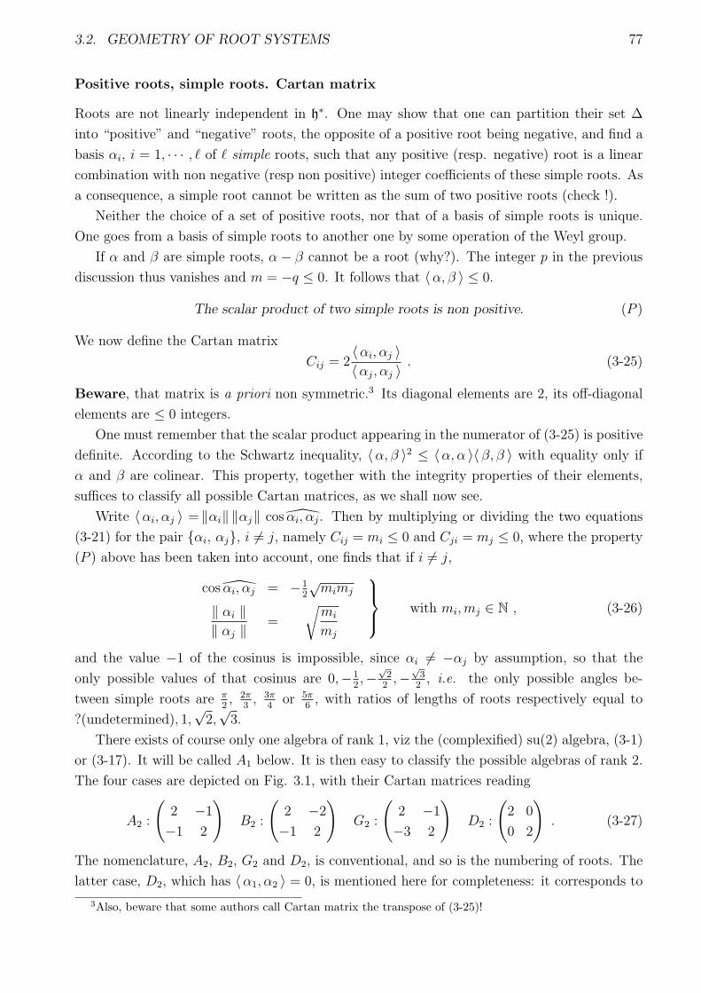
There exists of course only one algebra of rank 1, viz the (complexified) su(2) algebra, (3-1)

or (3-17). It will be called A1 below. It is then easy to classify the possible algebras of rank 2.

The four cases are depicted on Fig. 3.1, with their Cartan matrices reading

A2 :

!2 "1

"1 2

"B2 :

!2 "2

"1 2

"G2 :

!2 "1

"3 2

"D2 :

!2 0

0 2

". (3-27)

The nomenclature, A2, B2, G2 and D2, is conventional, and so is the numbering of roots. The

latter case, D2, which has )"1, "2 * = 0, is mentioned here for completeness: it corresponds to

3Also, beware that some authors call Cartan matrix the transpose of (3-25)!


D2

!!!!"!!!!#

!#

$!!!!!"#!!!!

#$

" !"$

!!!!"!!!!##

%$

!!!!"!#!!!!#

%!!!!!"!!!!#$

A B2 2

! !# $

!$

" !$

$!!!!"!!!!

#

!$

!# $

!!!!"!!!!#

#!!!!!"!!!!#$

!$

!#

G2

Figure 3.1: Root systems of rank 2. The two simple roots are drawn in thick lines. For the

algebras B2, G2 et D2, only positive roots have been labelled.

A

B

D

C

E

E

E

F

G

! " # l

! " # l

! " # l

l

l

l

l

7

6

8

! "

#

$ %

&

! "

#

$ % &

'

! "

#

$ % & '

(

! " $#

4

2

! "

! " #

l

l

!!

Figure 3.2: Dynkin diagrams

a semi-simple algebra, the direct sum of two A1 algebras. (Nothing forces its two roots to be

of equal length.)

In general, if the set of roots may be split into two mutually orthogonal subsets, one sees

that the Lie algebra decomposes into a direct sum of two algebras, and vice versa. Recalling

that any semi-simple algebra may be decomposed into the direct sum of simple subalgebras

(see end of Chap. 1), in the following we consider only simple algebras.

Dynkin diagram

For higher rank , i.e. for higher dimension of the root space, it becomes di#cult to visualise the

root system. Another representation is adopted, by encoding the Cartan matrix into a diagram

in the following way: with each simple root is associated a vertex of the diagram; two vertices

are linked by an edge i" )"i, "j * (= 0; the edge is simple if Cij = Cji = "1 (angle of 2&/3,

equal lengths); it is double (resp. triple) if Cij = "2 (resp. "3) and Cji = "1 (angle of 3$4

resp. 5$6 , with a length ratio of

/2, resp.

/3) and then carries an arrow (or rather a sign >)

from i to j indicating which root is the longest. (Beware that some authors use the opposite

convention for arrows !).


3.2.2 Root systems of simple algebras. Cartan classification

The analysis of all possible cases led Cartan4 to a classification of simple complex Lie algebras,

in terms of four infinite families and five exceptional cases. The traditional notation is the

following

A#, B#, C#, D#, E6, E7, E8, F4, G2 . (3-28)

In each case, the lower index gives the rank of the algebra. The geometry of the root system is

encoded in the Dynkin diagrams of Fig. 3.2.

The four infinite families are identified with the (complexified) Lie algebras of classical

groups

A# = sl(! + 1, C), B# = so(2! + 1, C), C# = sp(2!, C), D# = so(2!, C) . (3-29)

or with their unique compact real form, respectively A# = su(! + 1), B# = so(2! + 1),

C# = usp(!), D# = so(2!).The “exceptional algebras” E6, . . . , G2 have respective dimensions 78, 133, 248, 52 and 14. Those are

algebras of . . . exceptional Lie groups! The group G2 is the group of automorphisms of octonions, F4 is itself anautomorphism group of octonion matrices, etc.

Among these algebras, the algebras A, D, E, whose roots have the same length, are called simply laced. Acurious observation is that many problems, finite subgroups of su(2), “simple” singularities, “minimal conformalfield theories”, etc, are classified by the same ADE scheme. . . but this is another story!

The real forms of these simple complex algebras have also been classified by Cartan. One finds 12 infiniteseries and 23 exceptional cases!

3.2.3 Chevalley basis

There exists another basis of the Lie algebra g, called Chevalley basis, with brackets depending only on theCartan matrix. Let hi, ei et fi, i = 1, · · · , #, be generators attached to simple roots !i according to

ei =3

2)!i, !i *

4 12

E!i , fi =3

2)!i, !i *

4 12

E!!i , hi =2!i.H

)!i, !i *. (3-30)

Their commutation relations read

[hi, hj ] = 0[hi, ej ] = Cji ej

[hi, fj ] = "Cji fj

[ei, fj ] = $ijhj (3-31)

(check!). The algebra is generated by the ei, fi, hi and all their commutators, constrained by (3-31) and by the“Serre relations”

ad (ei)1!Cjiej = 0 (3-32)

ad (fi)1!Cjifj = 0 . (3-33)

This proves that the whole algebra is indeed encoded in the data of the simple roots and of their geometry(Cartan matrix or Dynkin diagram).

Note also the remarkable and a priori not obvious property that in that basis, all the structure constants(coe!cients of the commutation relations) are integers.

4This classification work, undertaken by Killing, was corrected and completed by E. Cartan, and latersimplified by van der Waerden, Dynkin, . . .


3.2.4 Coroots. Highest root. Coxeter number and exponents

We give here some complements on notations and concepts that are encountered in the study of simple Liealgebras and of their root systems.

As the combination!%i :=

2)!i, !i *

!i , (3-34)

for !i a simple root, appears frequently, it is given the name of coroot. The Cartan matrix may be rewritten as

Cij = )!i, !%j * . (3-35)

The highest root % is the positive root with the property that the sum of its components in a basis of simpleroots is maximal: one proves that this characterizes it uniquely. Its components in the basis of simple roots andin that of coroots

% =.

i

ai!i ,2

) %, % *% =.

i

a%i !%i , (3-36)

called Kac labels, resp dual Kac labels, play also a role, in particular through their sums,

h = 1 +.

i

ai , h% = 1 +.

i

a%i . (3-37)

The numbers h and h% are respectively the Coxeter number and the dual Coxeter number. When a normalisationof roots has to be picked, which we have not done yet, one usually imposes that ) %, % * = 2.

Lastly the diagonalisation of the symmetrized Cartan matrix

5Cij := 2)!i, !j *6

)!i, !i *)!j , !j *(3-38)

yields a spectrum of eigenvalues

eigenvalues of 5C =7

4 sin28 &

2hmi

9:, i = 1, · · · , # , (3-39)

in which a new set of integers mi appears, the Coxeter exponents, satisfying 1 + mi + h " 1 with possiblemultiplicities. These numbers are relevant for various reasons. They contain useful information on the Weylgroup. After addition of 1, (making them , 2), one gets the degrees of algebraically independent Casimiroperators, or the degrees where the Lie group has a non trivial cohomology, etc etc.

Examples: for An!1 alias su(n), roots and coroots coincide. The highest root is % =#

i !i, thus h =h% = n, the Coxeter exponents are 1, 2 · · · , n " 1. For Dn alias so(2n), roots and coroots are again identical,% = !1 + 2!2 + · · · + 2!n!2 + !n!1 + !n, h = 2n" 2, and the exponents are 1, 3, · · · , 2n" 3, n" 1, with n" 1double if n is even.

See Appendix F for Tables of data on the classical simple algebras.

3.3 Representations of semi-simple algebras

3.3.1 Weights. Weight lattice

We now turn our attention to representations of semi-simple algebras, with an approach par-

allel to that of previous sections. In what follows, “representation” means finite dimensional

irreducible representation. We also assume these representations to be unitary: this is the case

of interest for representations of compact groups. The elements of the Cartan subalgebra com-

mute among themselves, they also commute in any representation. Denoting with “bras” and

3.3. REPRESENTATIONS OF SEMI-SIMPLE ALGEBRAS 81

“kets” the vectors of that representation, and writing simply X (instead of d(X)) for the rep-

resentative of the element X % g, one may find a basis |#a * which diagonalises simultaneously

the elements of the Cartan algebra

H|#a * = #(H)|#a * (3-40)

or equivalently

Hi|#a * = #(i)|#a * , (3-41)

with an eigenvalue # which is again a linear form on the space h, hence an element of h",

the root space. Such a vector # = (#(i)) of h" is called a weight. Note that for a unitary

representation, the H are Hermitian, hence # is real-valued: the weights are real vectors of h".

As the eigenvalue # may occur with some multiplicity, we have appended the eigenvectors with

a multiplicity index a. The set of weights of a given representation forms in the space h" the

weight diagram of the representation, see Fig. 3.5 below for examples in the case of su(3).

The adjoint representation is a particular representation of the algebra whose weights are

the roots. The roots studied in the previous sections thus belong to the set of weights in h".

The vectors |#a * forming a basis of the representation, their total number, incuding the

multiplicity, equals the dimension of the representation space E. This space E contains rep-

resentation subspaces for each of the su(2) algebras that we identified in § 3.2, generated by

{H!, E!, E!!}. By the same argument as in § 2, one now show that any weight # satisfies

#", 2)#, " *)", " * = m# % Z , (3-42)

and conversely, it may be shown that any # % h" satisfying (3-42) is the weight of some finite

dimensional representation. One may thus use (3-42) as an alternative definition of weights.

To convince oneself that the weights of any representation satisfy (3-42), one may, like in § 3.2,

define the maximal chain of weights through #

# + p#", · · · , #, · · · , # + q#" p# + 0, q# , 0 ,

which form a representation of the su(2) subalgebra, and then show that m# = "p# " q#.Let p# be the smallest + 0 integer such that (E!!)|p

!||'a * (= 0, and q# the largest , 0 integer such that(E!)q! |'a * (= 0, H! has respective eigenvalues )', ! * + p#)!,! *, and )', ! * + q#)!,! * on these vectors.Expressing that the eigenvalues of 2H!/)!,! * are opposite integers, one finds

2q# + 2)', ! *)!,! * = 2j 2p# + 2

)', ! *)!,! * = "2j .

Subtracting these equations gives q# " p# = 2j, and the length of the chain is 2j + 1 (dimension of the spin j

representation of su(2)), while adding them to get rid of 2j, one has

2)', ! *)!,! * = "(q# + p#) =: m#, as announced in (3-42).

This chain is invariant under the action of the Weyl reflection w!. (This is a generalisation

of the Z2 symmetry of su(2) “multiplets” ("j,"j + 1, · · · , j " 1, j).) More generally the set

of weights is invariant under the Weyl group: if # is a weight of a representation, so is w!(#),


and one shows that they have the same multiplicity. The weight diagram of a representation is

thus invariant under the action of W .

The set of weights is split by the Weyl group W into “chambers”, whose number equals the

order of W . The chamber associated with the element w of W is the cone

Cw = {#|)w#, "i * , 0 , #i = 1, · · · , !} , (3-43)

where the "i are the simple roots. (This is not quite a partition, as some weights belong to

the “walls” between chambers.) The fundamental chamber is C1, corresponding to the identity

in W . The weights belonging to that fundamental chamber are called dominant weights. Any

weight may be brought into C1 by some operation of W : it is on the “orbit” (for the Weyl group)

of a unique dominant weight. Among the weights of a representation, at least one belongs to

C1.

On the other hand, from [Hi, E!] = "(i)E! follows that

HiE!|#a * = ([Hi, E!] + E!Hi)|#a * = ("(i) + #(i))E!|#a *

hence that E!|#a *, if non vanishing, is an eigenvector of weight # + ". Now, in an irreducible

representation, all vectors are obtained from one another by such actions of E!, and we conclude

that

' Two weights of the same (irreducible) representation di!er by a integer-coe"cient combination

of roots,

(but this combination is in general not a root).

One then introduces a partial order on weights of the same representation: ## > # if

## " # =#

i ni"i, with non negative (integer) coe#cients ni. Among the weights of that

representation, one proves there exists a unique highest weight $, which is shown to be of

multiplicity 1. The highest weight vector will be denoted |$* (with no index a). It is such that

for any positive root E!|$* = 0, (otherwise, it would not be the highest), hence q# = 0 in the

discussion above, and )$, "* = 12)", "*j > 0, $ is thus a dominant weight.

' The highest weight of a representation is a dominant weight, $ % C1.

This highest weight vector characterises the irreducible representation. (In the case of su(2),

this would be a vector |j, m = j *.) In other words, two representations are equivalent i" they

have the same highest weight.

One then introduces the Dynkin labels of the weight # by

#i = 2)#, "i *)"i, "i *

% Z (3-44)

with "i the simple roots. For a dominant weight, thus for any highest weight of a representation,

these indices are non negative, i.e. in N.

The fundamental weights $i satisfy by definition

2)$j, "i *)"i, "i *

= %ij . (3-45)


Their number equals the rank ! of algebra, and they make a basis of h". Each one is the high-

est weight of an irreducible representation called fundamental; hence there are ! fundamental

representations. We have thus obtained

' Any irreducible representation irreducible is characterised by its highest weight,

and with a little abuse of notation, we denote ($) the irreducible representation of highest

weight $.

' Any highest weight decomposes on fundamental weights, and its components are its Dynkin

labels (3-44),

$ =#.

j=1

#j$j , #i % N . (3-46)

and any $ of the form (3-46) is the highest weight of an irreducible representation.

Stated di"erently, the knowledge of the fundamental weight su#ces to construct all irreducible

representations of the algebra.Using the properties just stated, show that the highest weight of the adjoint representation is necessarily %,

defined in § 2.4.

Weight and root lattices

Generally speaking, given a basis of vectors e1, · · · ep in a p dimensional space, the lattice

generated by these vectors is the set of vectors#p

i=1 ziei with coe#cients zi % Z. This lattice

is also denoted Ze1 + · · · + Zep.

The weight lattice P is the lattice generated by the fundamental ! weights $i. The root

lattice Q is the one generated by the ! simple roots "i. This is a sublattice of P . Any weight

of an irreducible representation belongs to P .

One may consider the congruence classes of the additive group P wrt its subgroup Q, that

are the classes for the equivalence relation # 0 ## i" # " ## % Q. The number |P/Q| of these

classes turns out to be equal to the determinant of the Cartan matrix(!). In the case of su(n),

there are n classes, we shall return to that point later.

One may also introduce the lattice Q% generated by the # coroots !%i (cf §2.4). It is the “dual” of P , in thesense that )!%i ,"j * % Z.

One also shows that the subgroups of the finite group P/Q are isomorphic to homotopy groups of groupsG having g as a Lie algebra! For example for su(n), we find below that P/Q = Zn, and these subgroups arecharacterised by a divisor d of n. For each of them, SU(n)/Zd has the su(n) Lie algebra. The case n = 2, withSU(2) and SO(3), is quite familiar.

Dimension and Casimir operator

It may be useful to know the dimension of a representation with a given highest weight and the

value of the quadratic Casimir operator in that representation. These expressions are given in

terms of the Weyl vector (, defined by any of the two (non trivially!) equivalent formulas

( = 12

#!>0 "

=#

j $j . (3-47)


A remarkable formula, due to Weyl, gives the dimension of the representation of highest weight

$ as a product over positive roots

dim($) =;

!>0

)$ + (, " *) (, " * (3-48)

while the eigenvalue of the quadratic Casimir reads

C2($) =1

2)$, $ +2 ( * . (3-49)

A related question is that of the trace of generators of g in the representation ("). Let ta be the basisof g such that tr tatb = TA$ab, with a coe!cient TA (“A” like adjoint) whose sign depends on conventions (tHermitian or antiHermitian, see Chap. 1). In the representation of highest weight ", one has

tr d!(ta)d!(tb) = T!$ab . (3-50)

But in that basis, the quadratic Casimir reads C2 =#

a (d!(ta))2 hence, taking the trace,

trC2 =#

a tr (d!(ta))2 = T!#

a 1 = T! dim g

= C2(") tr I! = C2(") dim(") (3-51)

whenceT! = C2(")

dim(")dim g

, (3-52)

a useful formula in calculations (gauge theories . . . ). In the adjoint representation, dim(A) = dim g, henceT! = TA = C2(A).

There is a host of additional, sometimes intriguing, formulas relating various aspects of Lie algebras andrepresentation theory. For example the Freudenthal–de Vries “strange formula”, which connects the norms ofthe vectors ( and % to the dimension of the algebra and the Coxeter number: ) (, ( * = h

24 ) %, % *dim g.There is also a formula (Freudenthal) giving the multiplicity of a weight ' within a representation of given

highest weight ". And last, as a related issue, a formula by Weyl giving the character )!(eH) of that represen-tation evaluated on an element of the Cartan torus, an abelian subgroup resulting from the exponentiation ofthe Cartan algebra h.

Conjugate representation

Given a representation of highest weight ", its complex conjugate representation is generally non equivalent. Onmay characterize what is its highest weight " thanks to the Weyl group. The non-equivalence of representations(") and (") has to do with the symmetries of the Dynkin diagram. For the algebras of type B, C,E7, E8, F4, G2

for which there is no non trivial symmetry, the representations are self-conjugate. This is also the case of D2r.For the others, conjugation corresponds to the following symmetry on Dynkin labels

A# = su(# + 1) 'i - '#+1!i # > 1D2r+1 = so(4r + 2) '# - '#!1 , # = 2r + 1

E6 'i - '6!i, i = 1, 2 . (3-53)

3.3.2 Roots and weights of su(n)

Let us construct explicitly the weights and thus the irreducible representations of su(n).

We first pick a convenient parametrization of the space h", which is of dimension n" 1. Let

ei, i = 1, · · ·n, be n vectors of h" = Rn!1 (hence necessarily dependent), satisfying#n

1 ei = 0.


They are obtained starting from an orthonormal basis ei of Rn by projecting the ei on the

hyperplane orthogonal to ( :=#n

i=1 ei, thus ei = ei " 1n (. (In other words, one is considering

the hyperplane#n

i xi = 1 in the space Rn). These vectors have scalar products given by

) ei, ej * = %ij "1

n. (3-54)

In terms of these vectors, the positive roots of su(n)= An!1, whose number equals |!+| =

n(n" 1)/2, are

"ij = ei " ej , 1 + i < j + n , (3-55)

and the ! = n" 1 simple roots are

"i = "i i+1 = ei " ei+1 , 1 + i + n" 1 . (3-56)

These roots have been normalized by )", " * = 2. The sum of positive roots is easily computed

to be

2( = (n" 1)e1 + (n" 3)e2 + · · · + (n" 2i + 1)ei + · · ·" (n" 1)en

= (n" 1)"1 + 2(n" 2)"2 + · · · + i(n" i)"i + · · · + (n" 1)"n!1. (3-57)

One checks that the Cartan matrix is

Cij=)"i, "j * =

$&

'2 if i = j

"1 if i = j ± 1

in accord with the Dynkin diagram of type An!1, thus justifying (3-56). The fundamental

weights $i, i = 1, · · · , n" 1 are then readily written

$i =i.

j=1

ej , (3-58)

e1 = $1, ei = $i " $i!1 for i = 2, · · · , n" 1, en = "$n!1 (3-59)

with scalar products

)$i, $j * =i(n" j)

n, i + j . (3-60)

The Weyl group W 1 SN acts on roots and on weights by permuting the ei:

w % W - w % SN : w(ei) = ew(i) .

Dimension of the representation of weight $

Combining formulas (3-48) and (3-55), prove the following expression

dim(") =;

1&i<j&n

fi " fj + j " i

j " iou fi :=

n!1.

k=i

'k, fn = 0. (3-61)


0 !"

Figure 3.3: Weights of su(2). The positive parts of the weight (small dots) and root (big dots)

lattices.

Conjugate representations

If $ = (#1, · · · , #n!1) is the highest weight of an irreducible representation of su(n), $ =

(#n!1, · · · , #1) is that of the complex conjugate, generally inequivalent, representation (see

above in § 3.3.1). Note that neither the dimension, nor the value of the Casimir operator

distinguish the representations $ and $.

“n-ality”.

There are n congruence classes of P with respect to Q. They are distinguished by the value of

*(') := '1 + 2'2 + · · · + (n" 1)'n!1 mod n , (3-62)

to which one may give the unimaginative name of “n-ality”, by extension of the “triality” of su(3), see below.The elements of the root lattice thus have *(') = 0.

Examples of su(2) and su(3).

In the case of su(2), there is one fundamental weight $ = $1 and one positive root ", normalised

by )", " * = 2, hence )$, " * = 1, )$, $ * = 12 . Thus " = 2$, $ corresponds to the spin 1

2

representation, " to spin 1. The weight lattice and the root lattice are easy to draw, see Fig.

3.3. The Dynkin label #1 is identical to the integer 2j, the two congruence classes of P wrt Q

correspond to representations of integer and half-integer spin, the dimension dim($) = #1 +1 =

2j + 1 and the Casimir operator C2($) = 14#1(#1 + 2) = j(j + 1), in accord with well known

expressions.

For su(3), the weight lattice is triangular, see Fig. (3.4), on which the triality )(#) :=

#1 + 2#2 mod 3 has been shown and the fundamental weights and the highest weights of the

“low lying” representations have been displayed. Following the common use, representations

are referred to by their dimension5

dim($) =1

2(#1 + 1)(#2 + 1)(#1 + #2 + 2) , (3-63)

supplemented by a bar to distinguish a representation from its conjugate, whenever necessary.

The conjugate of representation of highest weight $ = (#1, #2) has highest weight $ =( #2, #1).

Only the representations lying on the bisector of the Weyl chamber are thus self-conjugate.Exercise. Compute the eigenvalue of the quadratic Casimir operator in terms of Dynkin labels '1, '2 using

the formulas (3-49) and (3-57).

5which may be ambiguous; for example, identify on Fig. (3.4) the weight of another representation ofdimension 15.


3 6 10

6

10

8 15

15 27

3

1

!

!

"!

""

e

ee3 2

1"

!

C

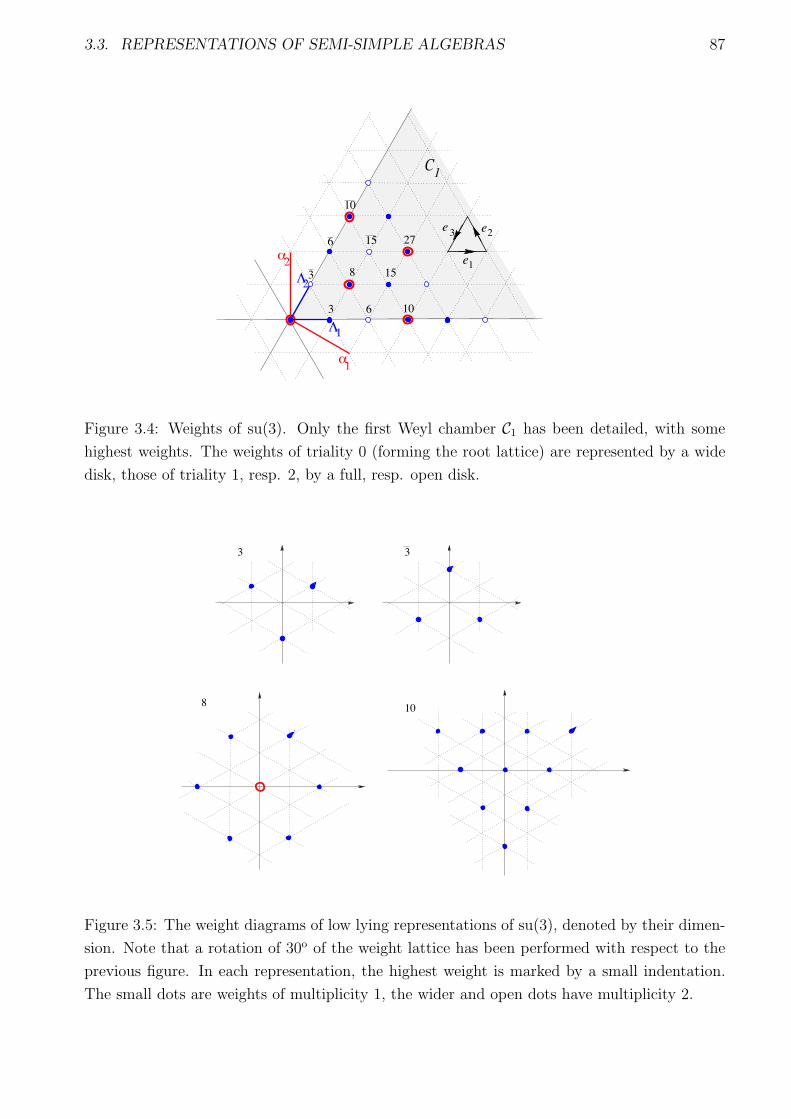
Figure 3.4: Weights of su(3). Only the first Weyl chamber C1 has been detailed, with some

highest weights. The weights of triality 0 (forming the root lattice) are represented by a wide

disk, those of triality 1, resp. 2, by a full, resp. open disk.

3

108

3

Figure 3.5: The weight diagrams of low lying representations of su(3), denoted by their dimen-

sion. Note that a rotation of 30o of the weight lattice has been performed with respect to the

previous figure. In each representation, the highest weight is marked by a small indentation.

The small dots are weights of multiplicity 1, the wider and open dots have multiplicity 2.


156

8 15

63

3

1

27

10

10

24

Figure 3.6: Tensor product of the 8 representation by the 3 representation, depicted on the

weight diagram of su(3).

The set of weights of low lying representations is displayed on Fig. (3.5), after a rotation

of the axes of the previous figures. The horizontal axis, colinear to "1, and the vertical axis,

colinear to $2, will indeed acquire a physical meaning: that of axes of isospin and “hypercharge”

coordinates, see next chapter.

Remark. The case of su(n) has been detailed. Analogous formulas for roots, fundamen-

tal weights, etc of other simple algebras are of course known explicitly and tabulated in the

literature. See for example Appendix F for the identity card of “classical algebras”, of type

A, B, C, D, and Bourbaki, chap.6, for more details on the other algebras.

3.4 Tensor products of representations of su(n)

3.4.1 Littlewood-Richardson rules

Given two irreducible representations of su(n) (or of any other Lie algebra), a frequently en-

countered problem is to decompose their tensor product into a direct sum of irreducible rep-

resentations. If one is only interested in multiplicities and if one has a character table of the

corresponding compact group, one may use the formulae proved in Chap. 2, § 2.3.2.

There exists also fairly complex rules giving that decomposition into irreducible represen-

tations of a product of two irreducible representations ($) and ($#) of su(n). Those are the

Littlewood-Richardson rules, which appeal to the expression in terms of Young tableaux (see

next §). But it is often simpler to proceed step by step, noticing that the irreducible represen-

tation ($#) is found in an adequate product of fundamental representations, and examining the

successive products of representation $ by these fundamental representations. By the associa-

tivity of the tensor product, one brings the original problem back to that of the tensor product

of ($) by the various fundamental representations.

The latter operation is easy to describe on the weight lattice. Given the highest weight $

in the first Weyl chamber C1, the tensor product of ($) by the fundamental representation of

highest weight $i is decomposed into irreducible representations in the following way: one adds

in all possible ways the dim($i) weights of the fundamental to the vector $ and one keeps as

highest weights in the decomposition only the weights resulting from this addition that belong

to C1.

chapter 3 simple lie algebras. classiﬁcation and representations. roots...

Documents