chapter 3 segmentation using modified fuzzy c-means...

45

CHAPTER 3

SEGMENTATION USING MODIFIED FUZZY C-MEANS

CLUSTERING WITH A GENETICALLY OPTIMIZED

APPROACH

3.1 INTRODUCTION

Spatial intensity inhomogeneity in MRI is a major problem in the

computer analysis of MRI data. Intensity inhomogeneity (also termed as the

intensity nonuniformity, the bias field, or the gain field in the literature) arises

from the imperfections of the image acquisition process and manifests itself

as a smooth intensity variation across the image. Because of this

phenomenon, the intensity of the same tissue varies with the location of the

tissue within the image. Although intensity inhomogeneity is in general

hardly noticeable to a human observer, many medical image analysis

methods, such as segmentation and registration, are highly sensitive to the

spurious variations of image intensities.

In this chapter, a novel approach is proposed for fuzzy

segmentation of MRI data in the presence of intensity inhomogeneities. The

proposed method simultaneously estimates the bias field while segmenting

the image. The algorithm is formulated by modifying the objective function of

the standard FCM algorithm to compensate for such inhomogeneities. This

allows the labeling of a pixel to be influenced by the labels in its immediate

neighborhood. The neighborhood effect acts as a regularizer and biases the

solution towards piecewise-homogeneous labeling: such regularization is

46

useful in segmenting scans corrupted by salt and pepper noise. Clustering

algorithms such as FCM, which use calculus-based optimization methods, can

be trapped by local extrema in the process of optimizing the clustering

criterion. They are also very sensitive to initialization. The proposed

algorithm uses GA to optimize the cluster centers in the modified fuzzy ( Jm )

c-means function to avoid local extrema. The performance of the algorithm is

evaluated on simulated and real MR images of the brain.

3.2 MODEL OF INTENSITY INHOMOGENEITY

The observed MRI signal is modeled as a product of the true signal

generated by the underlying anatomy, and a spatially varying factor called the

gain field

k k kY X G k 1, 2,.....N (3.1)

where kX and kY are the true and observed intensities at the kth pixel,

respectively. kG is the gain field at the kth pixel, and N is the total number of

pixels in the MR image.

The application of a logarithmic transformation to the intensities

allows the artifact to be modeled as an additive bias field.

k k ky x k 1,2,.....N (3.2)

where kx and ky are the true and observed log-transformed intensities at the

kth pixel, respectively. k is the bias field at the kth pixel. If the gain field is

known, then it is relatively easy to estimate the tissue class by applying a

47

conventional intensity-based segmenter to the corrected data. Similarly, if the

tissue classes are known, then the gain field can be estimated, but it may be

problematic to estimate either without the knowledge of the other. The tissue

classes and the gain field can be estimated by using an iterative algorithm

based on fuzzy logic.

3.3 FUZZY C-MEANS CLUSTERING

The FCM clustering algorithm assigns a fuzzy membership value to

each data point based on its proximity to the cluster centroids in the feature

space. FCM is a clustering algorithm, but the resulting partition is fuzzy. The

input feature vectors are not assigned exclusively to a single class, but

partially to all classes. If a single class must be chosen, the data point chosen

should be in the class with the higher membership grade. This is called

defuzzification and yields a crisp label. The FCM algorithm assumes that the

number of clusters c is known and minimizes the objective function to find

the best set of cluster centers. The standard FCM objective function for

partitioning 1

Nk k

x

into c clusters is given by

2

1 1

c N pJ u x viik ki k

(3.3)

where 1

ci i

v

are the prototypes of the clusters and the array [ iku ] = U

represents a partition matrix, U u , namely

u 0,1iku 1

1 c

iki

u k

and 0 < 1

N

ikk

u < N i (3.4)

48

The parameter p is a weighing exponent on each fuzzy membership

and determines the amount of fuzziness of the resulting classification. The

FCM objective function is minimized when high membership values are

assigned to pixels whose intensities are close to the centroid of its particular

class, and low membership values are assigned when the pixel data are far

from the centroid.

Given a partition, the cluster centers are calculated using

1

1

, 1

Np

ik kk

i Np

ikk

u xv i c

u

(3.5)

The iteration is then completed by calculating the new partition:

12 / 1

1, 1 , 1

pc

k iik

j k j

x vu i c k N

x v (3.6)

The FCM algorithm for segmenting the image into different

clusters can be summarized in the following steps.

Step1 : Fix c (2…..c<n) and select a value for parameter p and

initialize the cluster centers 1

ci i

v

.

Step2 : Calculate the partition matrix U using equation (3.6).

Step 3 : Update the c centers 1

ci i

v

for each step using

equation (3.5).

49

Step4 : Repeat Step 2-3 till termination. The termination

criterion is as follows:

V Vnew old (3.7)

where . is the Euclidean norm, V is a vector of cluster centers, and is a

small number that can be set by the user.

3.4 BIAS CORRECTED FUZZY C-MEANS (BCFCM)

OBJECTIVE FUNCTION

The standard FCM objective function given in equation (3.3) is

modified by introducing a term that allows the labeling of a pixel to be

influenced by the labels in its immediate neighborhood (Ahmed et al 1999).

The neighborhood effect acts as a regularizer and biases the solution towards

piecewise- homogeneous labeling. Such regularization is useful in segmenting

scans corrupted by salt and pepper noise. The modified objective function is

given by

22

1 11 1 r k

m r ix NR

c N c Np pJ u x v uiik k iki ik kx v

N

(3.8)

where kN stands for the set of neighbors that exist in a window around kx ,

and RN is the cardinality of Nk. The effect of the neighbor’s term is controlled

by the parameter . The relative importance of the regularizing term is

inversely proportional to the SNR of the MRI signal. Lower SNR would

require a higher value of the parameter . Substituting equation (3.2) into

equation (3.8).

50

2 2

1 11 1

c N c Np pJ u y v u y vm r ri iik k k ikN y Ni ik k rR k

(3.9)

Formally, the optimization problem comes in the form

1 1

min , subject to

, ,m

c Ni ki k

J U

U v

u

(3.10)

3.5 PARAMETER ESTIMATION

The objective function mJ can be minimized in a fashion similar to

the standard FCM algorithm. Taking the first derivatives of mJ with respect to

iku , iv and k , and setting them to zero results in three necessary but not

sufficient conditions for mJ to be at a local extrema. In the following

subsections, these three conditions are derived.

3.5.1 Membership Evaluation

The constrained optimization in equation (3.10) is solved using one

Lagrange multiplier

( ) (1 )1 11

c N cp pF u D u um iNik ik ik iki ik R

(3.11)

where, 2

ik ik kD y v and 2

(r k

i y N r r iy v

. The first

derivative of mF with respect to iku is taken and the result is set to zero, for

p >1

51

*

1 0ik ik

p pmik ik ik i

ik R u u

F ppu D uu N

(3.12)

Solving for iku

1( 1)

*

( )

p

ik

ik iR

up D

N

(3.13)

Since 1

1c

jkj

u

k

1( 1)

11

( )

p

c

jjk j

R

p DN

(3.14)

11( 1)

1

1

( )

p

p

c

jjk j

R

p

DN

(3.15)

Substituting into equation (3.13), the zero-gradient condition for

the membership estimator can be rewritten as

1( 1)

1

1ik

p

ik icR

jjk j

R

u

DN

DN

(3.16)

52

3.5.2 Cluster Prototype Updating

The following derivation, uses the standard Euclidean distance. The

derivative of mF with respect to iv is taken and the result is set to zero.

*1 1

0r k i i

N Np p

ik k k i ik r r ik k y NR v v

u y v u y vN

(3.17)

1

11

r k

Np

ik k k r rk y NR

Nip

ikk

u y yN

uv

(3.18)

3.5.3 Bias-Field Estimation

In a similar fashion, the derivative of mF with respect to k is taken

and the result is set to zero

*

2

1 10

k k

c Npik k k i

i kk

u y v

(3.19)

Since only the kth term in the second summation depends on k ,

the equation (3.19) is written as

*

2

10

k k

cpik k k i

i k

u y v

(3.20)

Differentiating the distance expression,

*

1 1 10

k k

c c cp p p

k ik k ik ik ii i i

y u u u v

(3.21)

53

Thus, the zero gradient condition for the bias field estimator is

expressed as

1

1

cp

ik ii

k ckp

iki

u vy

u

(3.22)

3.5.4 BCFCM Algorithm

The BCFCM algorithm for correcting the bias field and segmenting

the image into different clusters can be summarized in the following steps.

Step1 : Select initial class prototypes 1

ci i

v

. Set 1

Nk k

to equal

and very small values (e.g. 0.01).

Step2 : Update the partition matrix using equation (3.16).

Step3 : The prototypes of the clusters are obtained in the form of

weighted averages of the patterns using equation (3.18).

Step 4 : Estimate the bias term using equation (3.22).

Step5 : Repeat Step 2-4 till termination. The termination

criterion is as follows:

V Vnew old (3.23)

where . is the Euclidean norm, V is a vector of cluster centers, and is a

small number that can be set by the user.

54

3.6 GENETICALLY GUIDED CLUSTERING

Initialization has a significant effect on the final partitions obtained

by iterative c-means clustering approaches. The genetically guided clustering

attempts to achieve both avoidance of local extrema and minimal sensitivity

to initialization. On datasets with several local extrema, the GA approach

always avoids the less desirable solutions. In any generation, element i of the

population is Vi, a c s matrix of cluster centers in FCM. The cluster centers

and features are represented by c and s respectively. The initial population of

size P is constructed by a random assignment of real numbers to each of the s

features of the c cluster centers. The initial values are constrained to be in the

range of the feature to which they are assigned, but are otherwise random.

Since only the V’s will be used within the GA it is necessary to reformulate

the objective functions in equations (3.3) and (3.9) for optimization.

Case 1: FCM

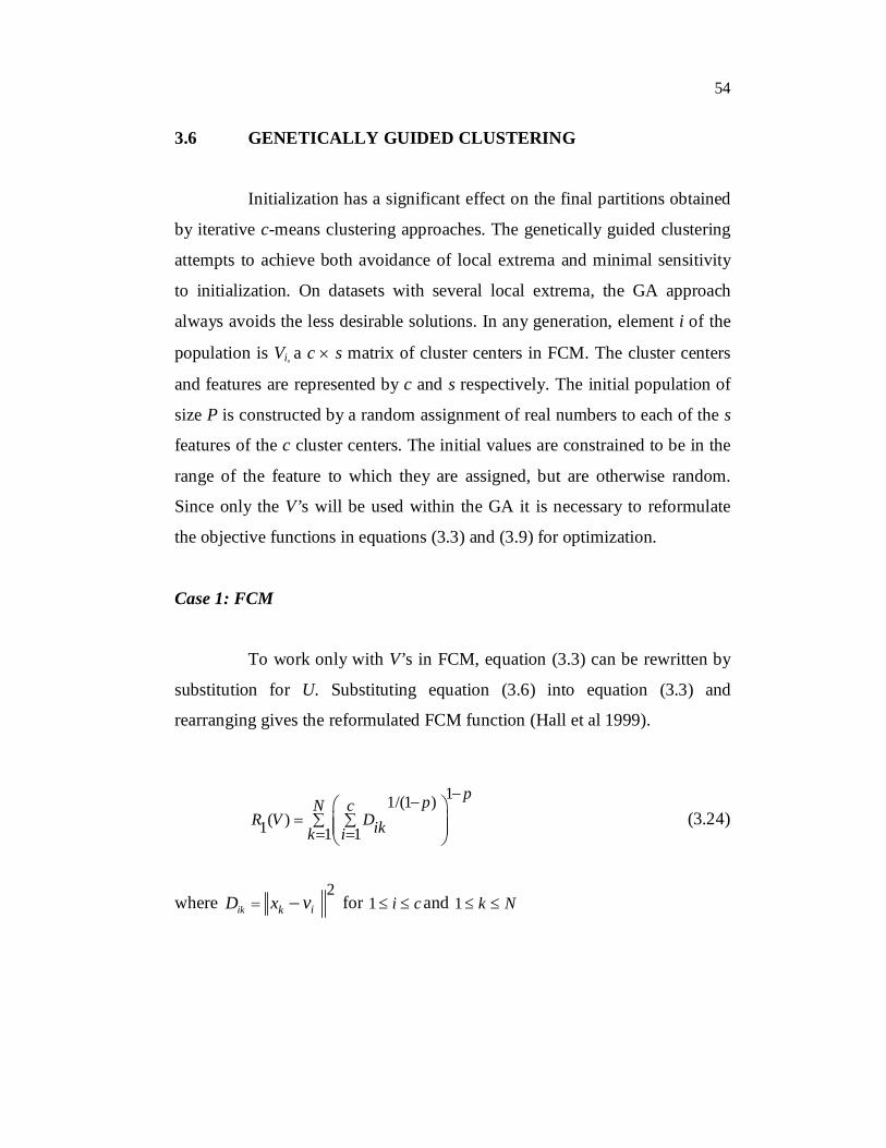
To work only with V’s in FCM, equation (3.3) can be rewritten by

substitution for U. Substituting equation (3.6) into equation (3.3) and

rearranging gives the reformulated FCM function (Hall et al 1999).

11/(1 )

( )1 11

ppN cR V Dikik

(3.24)

where 2

ik ikD x v for 1 i c and 1 k N

55

Case 2: BCFCM

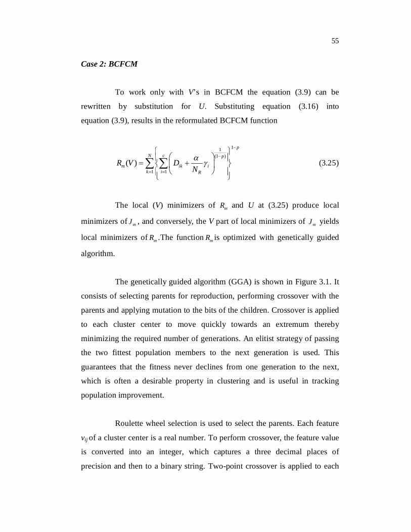
To work only with V’s in BCFCM the equation (3.9) can be

rewritten by substitution for U. Substituting equation (3.16) into

equation (3.9), results in the reformulated BCFCM function

11(1 )

1 1( )

p

N c p

m ik ik i R

R V DN

(3.25)

The local (V) minimizers of mR and U at (3.25) produce local

minimizers of mJ , and conversely, the V part of local minimizers of mJ yields

local minimizers of mR .The function mR is optimized with genetically guided

algorithm.

The genetically guided algorithm (GGA) is shown in Figure 3.1. It

consists of selecting parents for reproduction, performing crossover with the

parents and applying mutation to the bits of the children. Crossover is applied

to each cluster center to move quickly towards an extremum thereby

minimizing the required number of generations. An elitist strategy of passing

the two fittest population members to the next generation is used. This

guarantees that the fitness never declines from one generation to the next,

which is often a desirable property in clustering and is useful in tracking

population improvement.

Roulette wheel selection is used to select the parents. Each feature

vij of a cluster center is a real number. To perform crossover, the feature value

is converted into an integer, which captures a three decimal places of

precision and then to a binary string. Two-point crossover is applied to each

56

of the cluster centers of the mating parents generating two offspring. After

every crossover, each bit of the children is considered for mutation, with a

mutation probability pm. Mutation consists of flipping the value of the chosen

bit from 1 to 0 or vice versa.

Step1: Choose p and c.

Step2: Randomly initialize P sets of c cluster centers. Constrain the initial

values to be within the space defined by the vectors to be clustered.

Step3: Calculate R1 or mR using equation (3.24) or (3.25) for each

population member.

Step4: For 1i to number of generations do

Use Roulette wheel selection to select parents for reproduction.

Do two-point crossover and bit wise mutation on each feature of

the parent pairs.

Calculate R1 or Rm using equation (3.24) or (3.25) for each

population member.

Create the new generation of size P from the 2 best members of

the previous generation and the best children that resulted from

crossover and mutation.

Figure 3.1 The genetically guided algorithm

3.7 RESULTS AND DISCUSSION

The simulated and real MR brain images are used for validating the

segmentation methods. The 20 simulated brain images are obtained from

Brainweb database at the Mc Connell Brain Imaging Center of the Montreal

Neurological Institute, McGill University (Cocosco et al 1997, Kwan et al

1999, Collins et al 1998). This site also provides the ground-truth that enables

57

one to obtain a quantitative assessment of the performance of the algorithm.

This database contains a set of realistic MRI data volumes produced by an

MRI simulator. It provides full 3-dimensional data volumes using three

sequences (T1-, T2-, and proton-density- (PD-) weighted) and a variety of

slice thicknesses, noise levels, and levels of intensity non-uniformity. These

data are available for viewing in three orthogonal views (transversal, sagittal,

and coronal). T1 weighted MR brain images in axial view are used in this

work for segmentation.

The cerebrum is extracted from the brain images using

morphological image processing techniques before applying the clustering

algorithm. In the implementation of BCFCM, parameter is set as 0.7, p=2,

NR =9 (3 3 window centered around each pixel) and ε =0.01. For low SNR

images is set as 0.85. The FCM/BCFCM algorithm gets trapped in local

extrema when initial clusters are not properly chosen. In 50 runs of

FCM/BCFCM with random initializations of cluster centers, all of them

apparently result in degenerate partitions consisting of just one class. To

obtain some nondegenerate partitions a different type of less random

initialization is used. In this initialization scheme, the cluster centers are

constrained to be in the range of the feature to which they are assigned. This

forces each cluster center to be distinct.

The GGA is used to optimize FCM and BCFCM. A population of

twenty chromosomes is randomly generated. Each center is represented in

8 bits. Roulette wheel selection method is used to select the mating pool,

which holds the parents that generate offspring. Two point crossover is

applied to the cluster centers of the mating parents generating two offspring

with a crossover probability pc=0.9. After every crossover, each bit of the

children is considered for mutation with a mutation probability pm=0.01.

58

The fitness function is inverse of R1(V) in case of GGFCM and inverse of

Rm(V) in case of GGBCFCM. The number of generations is used as the

stopping criteria for GGA.

The segmentation algorithms are run for various levels of noise and

intensity inhomogeneity. The Gaussian noise in the simulated images has

Rayleigh statistics in the background and Rician statistics in the signal regions.

The “percent noise” number represents the percent ratio of the standard

deviation of the white Gaussian noise versus the signal for a reference tissue

(white matter). For a 20% level of intensity inhomogeneity, the multiplicative

field has a range of values of 0.90 … 1.10 over the brain area. For other

intensity inhomogeneity levels, the field is linearly scaled accordingly (for

example, to a range of 0.80 … 1.20 for a 40% level).

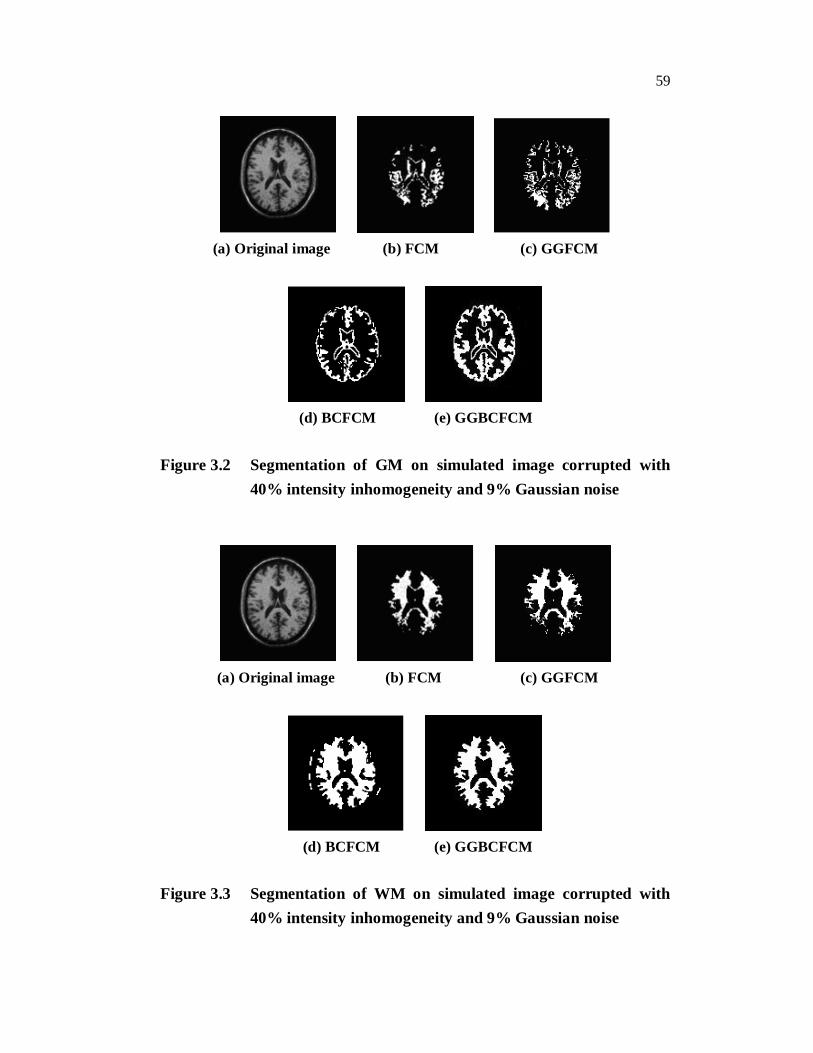
The segmentation results of FCM, GGFCM, BCFCM and

GGBCFCM when applied on T1 weighted simulated MR image corrupted

with 40% intensity inhomogeneity and 9% Gaussian noise are presented in

Figures 3.2 to 3.5. The clustering algorithms segment the image into four

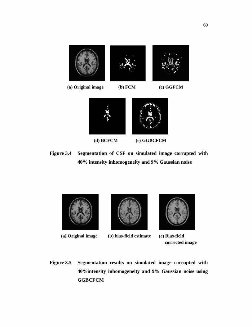
classes corresponding to GM, WM, CSF, and background. Figure 3.5(b)

shows the estimate of the multiplicative gain. This image was obtained by

scaling the values of the bias field from one to 255. Figure 3.5(c) depicts the

corrected image.

59

(a) Original image (b) FCM (c) GGFCM

(d) BCFCM (e) GGBCFCM Figure 3.2 Segmentation of GM on simulated image corrupted with

40% intensity inhomogeneity and 9% Gaussian noise


(d) BCFCM (e) GGBCFCM Figure 3.3 Segmentation of WM on simulated image corrupted with


60


(d) BCFCM (e) GGBCFCM

Figure 3.4 Segmentation of CSF on simulated image corrupted with


(a) Original image (b) bias-field estimate (c) Bias-field corrected image

Figure 3.5 Segmentation results on simulated image corrupted with

40%intensity inhomogeneity and 9% Gaussian noise using

GGBCFCM

61

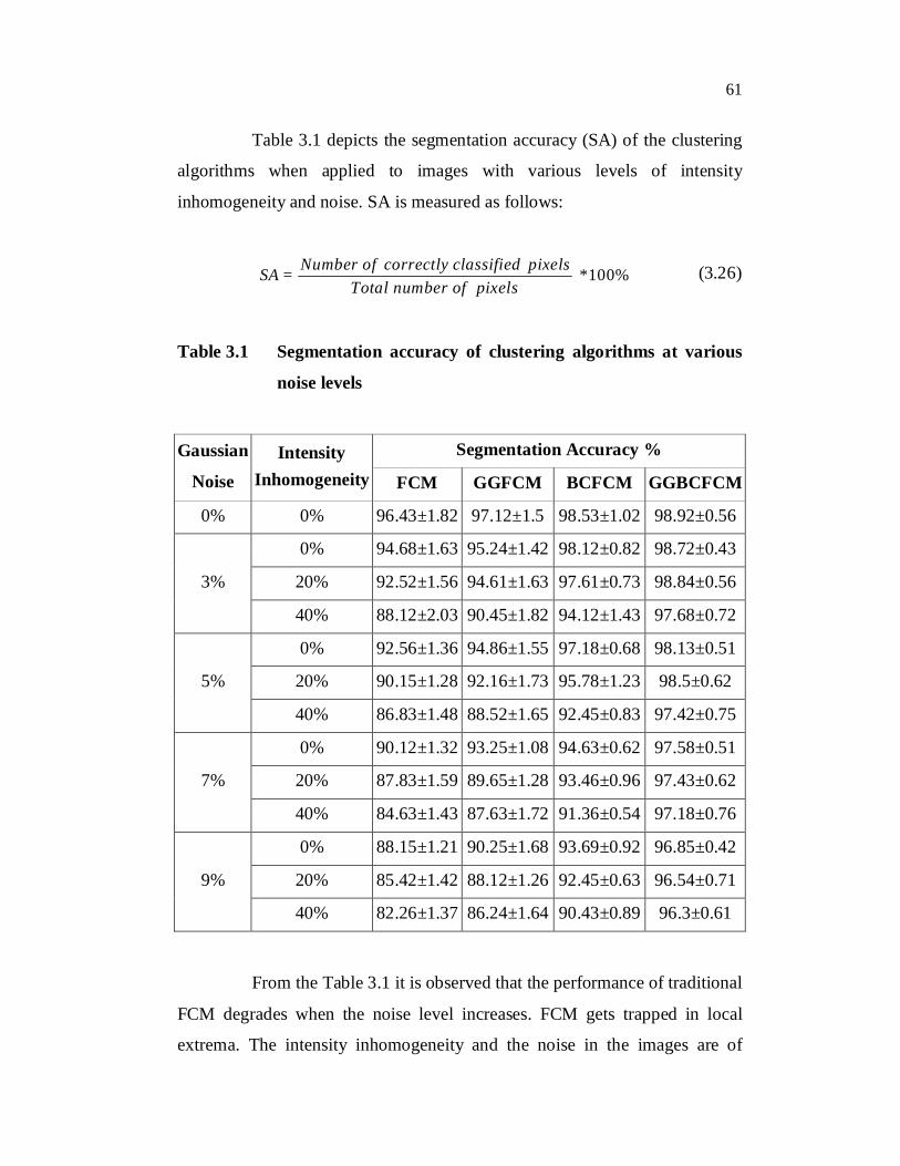
Table 3.1 depicts the segmentation accuracy (SA) of the clustering

algorithms when applied to images with various levels of intensity

inhomogeneity and noise. SA is measured as follows:

*100%Number of correctly classified pixelsSA =Total number of pixels

(3.26)

Table 3.1 Segmentation accuracy of clustering algorithms at various

noise levels

Gaussian

Noise Intensity

Inhomogeneity

Segmentation Accuracy %

FCM GGFCM BCFCM GGBCFCM

0% 0% 96.43±1.82 97.12±1.5 98.53±1.02 98.92±0.56

3%

0% 94.68±1.63 95.24±1.42 98.12±0.82 98.72±0.43

20% 92.52±1.56 94.61±1.63 97.61±0.73 98.84±0.56

40% 88.12±2.03 90.45±1.82 94.12±1.43 97.68±0.72

5%

0% 92.56±1.36 94.86±1.55 97.18±0.68 98.13±0.51

20% 90.15±1.28 92.16±1.73 95.78±1.23 98.5±0.62

40% 86.83±1.48 88.52±1.65 92.45±0.83 97.42±0.75

7%

0% 90.12±1.32 93.25±1.08 94.63±0.62 97.58±0.51

20% 87.83±1.59 89.65±1.28 93.46±0.96 97.43±0.62

40% 84.63±1.43 87.63±1.72 91.36±0.54 97.18±0.76

9%

0% 88.15±1.21 90.25±1.68 93.69±0.92 96.85±0.42

20% 85.42±1.42 88.12±1.26 92.45±0.63 96.54±0.71

40% 82.26±1.37 86.24±1.64 90.43±0.89 96.3±0.61

From the Table 3.1 it is observed that the performance of traditional

FCM degrades when the noise level increases. FCM gets trapped in local

extrema. The intensity inhomogeneity and the noise in the images are of

62

sufficient magnitude and cause the distributions of signal intensities

associated with the tissue classes to overlap significantly. GGFCM slightly

improves the performance of FCM. BCFCM which uses the neighborhood

effect is better than GGFCM.

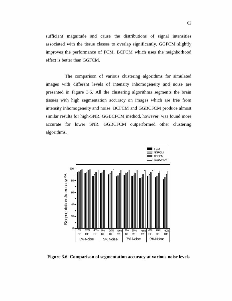
The comparison of various clustering algorithms for simulated

images with different levels of intensity inhomogeneity and noise are

presented in Figure 3.6. All the clustering algorithms segments the brain

tissues with high segmentation accuracy on images which are free from

intensity inhomogeneity and noise. BCFCM and GGBCFCM produce almost

similar results for high-SNR. GGBCFCM method, however, was found more

accurate for lower SNR. GGBCFCM outperformed other clustering

algorithms.

0

20

40

60

80

100

9% Noise7% Noise5% Noise3% Noise

40% RF

20% RF

0% RF

40% RF

20% RF

0% RF

40% RF

20% RF

0% RF

40% RF

20% RF

0% RF

Segm

enta

tion

Accu

racy

%


Figure 3.6 Comparison of segmentation accuracy at various noise levels

63

The 20 real MRI brain data sets and their manual segmentation are

obtained from the Internet Brain Segmentation repository (IBSR) (IBSR

2004) of the Center for Morphometric Analysis at Massachusetts General

Hospital. The coronal three-dimensional T1-weighted spoiled gradient echo

MRI scans were performed on two different imaging systems. Ten Fast low-

angle shot (FLASH) scans on four males and six females were performed on a

1.5 tesla Siemens Magnetom MR System with the following parameters: TR

= 40 msec, TE = 8 msec, flip angle = 50 degrees, field of view = 30 cm, slice

thickness = contiguous 3.1 mm, matrix = 256 256. Ten scans on six males

and four females were performed on a 1.5 tesla General Electric Signa MR

System, with the following parameters: TR = 50 msec, TE = 9 msec, flip

angle = 50 degrees, field of view = 24 cm, slice thickness = contiguous

3.0mm, matrix = 256 256. Several researchers have used the Brainweb and

IBSR database as benchmark to validate their segmentation methods (Kapur

et al 1996, Cocosco et al 2003, Peng et al 2005, Ferreira da silva 2007).

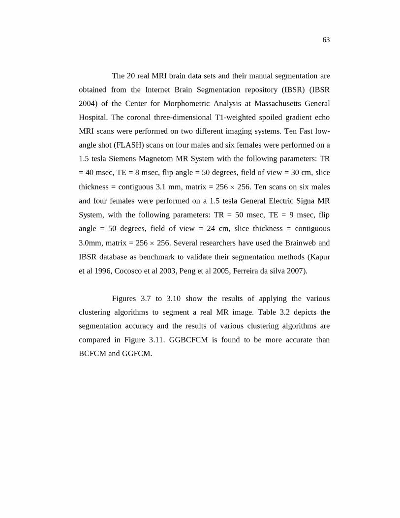
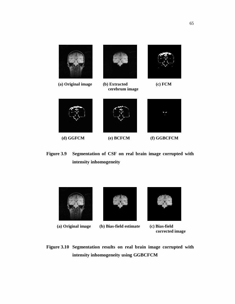
Figures 3.7 to 3.10 show the results of applying the various

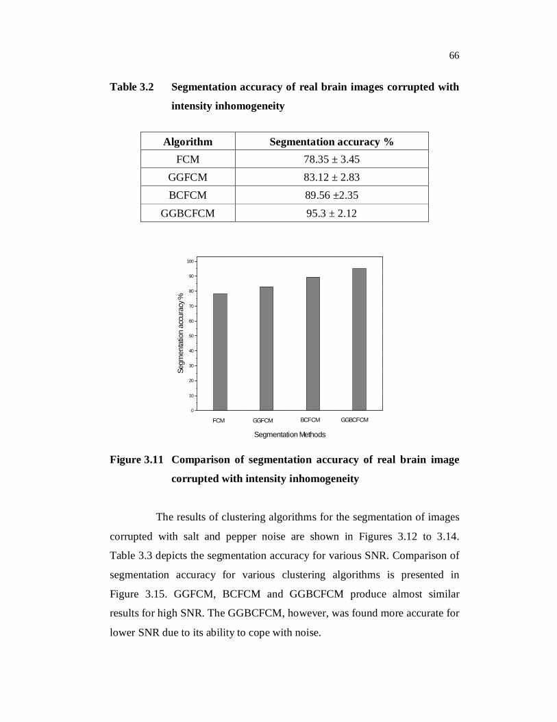
clustering algorithms to segment a real MR image. Table 3.2 depicts the

segmentation accuracy and the results of various clustering algorithms are

compared in Figure 3.11. GGBCFCM is found to be more accurate than

BCFCM and GGFCM.

64

(a) Original image (b) Extracted (c) FCM cerebrum image

(d) GGFCM (e) BCFCM (f) GGBCFCM

Figure 3.7 Segmentation of GM on real brain image corrupted with intensity inhomogeneity


(d) GGFCM (e) BCFCM (f) GGBCFCM Figure 3.8 Segmentation of WM on real brain image corrupted with

intensity inhomogeneity

65


(d) GGFCM (e) BCFCM (f) GGBCFCM

Figure 3.9 Segmentation of CSF on real brain image corrupted with


(a) Original image (b) Bias-field estimate (c) Bias-field corrected image

Figure 3.10 Segmentation results on real brain image corrupted with

intensity inhomogeneity using GGBCFCM

66

Table 3.2 Segmentation accuracy of real brain images corrupted with


Algorithm Segmentation accuracy % FCM 78.35 ± 3.45

GGFCM 83.12 ± 2.83 BCFCM 89.56 ±2.35

GGBCFCM 95.3 ± 2.12

0

10

20

30

40

50

60

70

80

90

100

GGBCFCMBCFCMGGFCMFCM

Segm

enta

tion

accu

racy

%

Segmentation Methods

Figure 3.11 Comparison of segmentation accuracy of real brain image

corrupted with intensity inhomogeneity

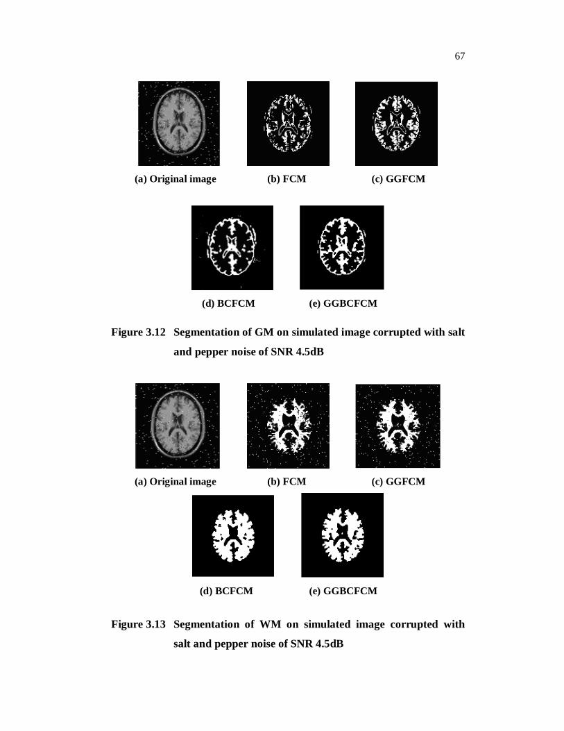
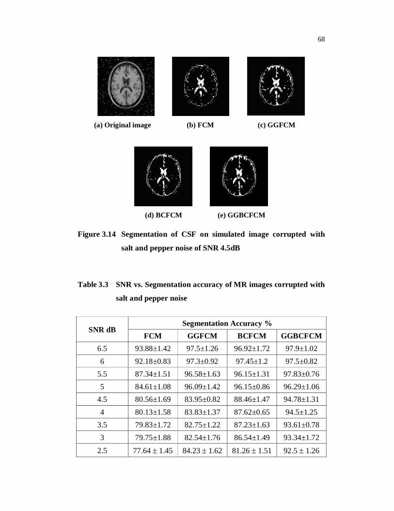
The results of clustering algorithms for the segmentation of images

corrupted with salt and pepper noise are shown in Figures 3.12 to 3.14.

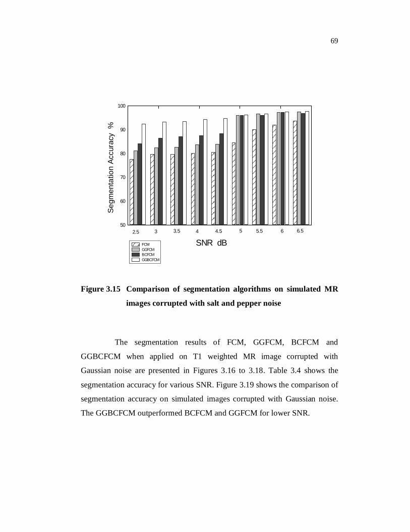
Table 3.3 depicts the segmentation accuracy for various SNR. Comparison of

segmentation accuracy for various clustering algorithms is presented in

Figure 3.15. GGFCM, BCFCM and GGBCFCM produce almost similar

results for high SNR. The GGBCFCM, however, was found more accurate for

lower SNR due to its ability to cope with noise.

67



Figure 3.12 Segmentation of GM on simulated image corrupted with salt

and pepper noise of SNR 4.5dB



Figure 3.13 Segmentation of WM on simulated image corrupted with

salt and pepper noise of SNR 4.5dB

68




salt and pepper noise of SNR 4.5dB

Table 3.3 SNR vs. Segmentation accuracy of MR images corrupted with

salt and pepper noise

SNR dB Segmentation Accuracy %

FCM GGFCM BCFCM GGBCFCM 6.5 93.88±1.42 97.5±1.26 96.92±1.72 97.9±1.02 6 92.18±0.83 97.3±0.92 97.45±1.2 97.5±0.82

5.5 87.34±1.51 96.58±1.63 96.15±1.31 97.83±0.76 5 84.61±1.08 96.09±1.42 96.15±0.86 96.29±1.06

4.5 80.56±1.69 83.95±0.82 88.46±1.47 94.78±1.31 4 80.13±1.58 83.83±1.37 87.62±0.65 94.5±1.25

3.5 79.83±1.72 82.75±1.22 87.23±1.63 93.61±0.78 3 79.75±1.88 82.54±1.76 86.54±1.49 93.34±1.72

2.5 77.64 1.45 84.23 1.62 81.26 1.51 92.5 1.26

69

50

60

70

80

90

100

6.565.554.543.532.5

Segm

enta

tion

Accu

racy

SNR dB FCM GGFCM BCFCM GGBCFCM

Figure 3.15 Comparison of segmentation algorithms on simulated MR

images corrupted with salt and pepper noise

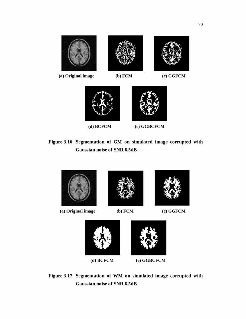
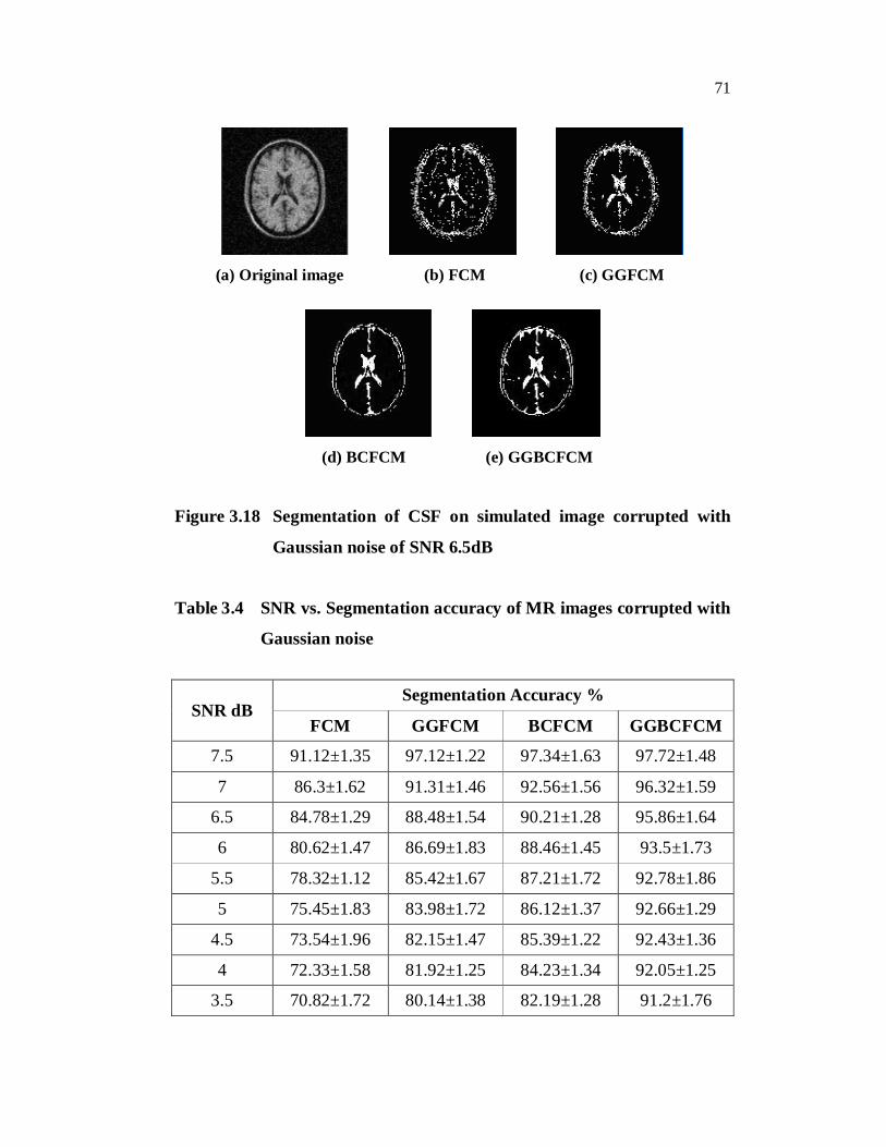
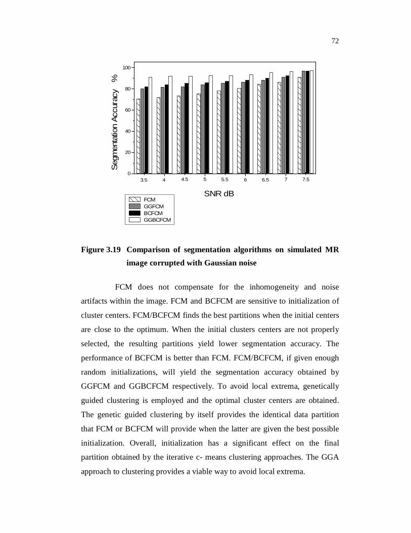
The segmentation results of FCM, GGFCM, BCFCM and

GGBCFCM when applied on T1 weighted MR image corrupted with

Gaussian noise are presented in Figures 3.16 to 3.18. Table 3.4 shows the

segmentation accuracy for various SNR. Figure 3.19 shows the comparison of

segmentation accuracy on simulated images corrupted with Gaussian noise.

The GGBCFCM outperformed BCFCM and GGFCM for lower SNR.

Segm

enta

tion

Accu

racy

%

70


(d) BCFCM (e) GGBCFCM Figure 3.16 Segmentation of GM on simulated image corrupted with

Gaussian noise of SNR 6.5dB


(d) BCFCM (e) GGBCFCM Figure 3.17 Segmentation of WM on simulated image corrupted with


71





Table 3.4 SNR vs. Segmentation accuracy of MR images corrupted with

Gaussian noise

SNR dB Segmentation Accuracy %


7.5 91.12±1.35 97.12±1.22 97.34±1.63 97.72±1.48

7 86.3±1.62 91.31±1.46 92.56±1.56 96.32±1.59

6.5 84.78±1.29 88.48±1.54 90.21±1.28 95.86±1.64

6 80.62±1.47 86.69±1.83 88.46±1.45 93.5±1.73

5.5 78.32±1.12 85.42±1.67 87.21±1.72 92.78±1.86

5 75.45±1.83 83.98±1.72 86.12±1.37 92.66±1.29

4.5 73.54±1.96 82.15±1.47 85.39±1.22 92.43±1.36

4 72.33±1.58 81.92±1.25 84.23±1.34 92.05±1.25

3.5 70.82±1.72 80.14±1.38 82.19±1.28 91.2±1.76

72

0

20

40

60

80

100

7.576.565.554.543.5

Segm

enta

tion

Accu

racy

%

SNR dB FCM GGFCM BCFCM GGBCFCM

Figure 3.19 Comparison of segmentation algorithms on simulated MR image corrupted with Gaussian noise

FCM does not compensate for the inhomogeneity and noise

artifacts within the image. FCM and BCFCM are sensitive to initialization of

cluster centers. FCM/BCFCM finds the best partitions when the initial centers

are close to the optimum. When the initial clusters centers are not properly

selected, the resulting partitions yield lower segmentation accuracy. The

performance of BCFCM is better than FCM. FCM/BCFCM, if given enough

random initializations, will yield the segmentation accuracy obtained by

GGFCM and GGBCFCM respectively. To avoid local extrema, genetically

guided clustering is employed and the optimal cluster centers are obtained.

The genetic guided clustering by itself provides the identical data partition

that FCM or BCFCM will provide when the latter are given the best possible

initialization. Overall, initialization has a significant effect on the final

partition obtained by the iterative c- means clustering approaches. The GGA

approach to clustering provides a viable way to avoid local extrema.

73

In this work, genetically guided bias corrected fuzzy c-means

algorithm is proposed for segmentation of MR images. This method

simultaneously estimates the bias field while segmenting the image. The

segmentation algorithms are run for various levels of intensity inhomogeneity

and Gaussian noise. The performance of FCM, GGFCM, BCFCM and

GGBCFCM is compared. For various noise levels, GGBCFCM segments the

brain tissues with higher degree of accuracy and estimates the bias field

accurately. The results using simulated MR and real brain images show that

intensity variations across patients, scans and equipment changes have been

accommodated in the estimated bias field without the need for manual

intervention.

chapter 3 segmentation using modified fuzzy c-means...

Documents