chapter 3 programming with matlab. newton’s second law euler’s method to obtain good...

Chapter 3Chapter 3

Programming with Programming with MATLABMATLAB

Newton’s Second Law

Euler’s method

To obtain good accuracy, it is necessary to use many small steps

Extremely laborious and time-consuming to implement by hand

Numerical SolutionNumerical Solution

2d2d v

m

cg

dt

dvvcmg

dt

dvm

)()()()( i1i2

id

i1i tttvm

cgtvtv

M-Files: Scripts and FunctionsM-Files: Scripts and Functions You can create and save code in text files using

MATLAB Editor/Debugger or other text editors (called m-files since the ending must be .m)

M-file is an ASCII text file similar to FORTRAN or C source codes ( computer programs)

A script can be executed by typing the file name, or using the “run” command

Difference between scripts and functionsDifference between scripts and functions

Scripts share variables with the main workspace

Functions do not

Script FilesScript Files

Script file – a series of MATLAB commands saved on a file, can be executed by

typing the file name in the Command Window invoking the menu selections in the Edit Window:

Debug, Run

Create a script file using menu selection:

File, New, M-file

Compute the velocity of a free-falling bungee jumper at a specific time

Open the editor with: File, New, M-file

Save the file as bungee_jumper.m Type bungee_jumper in command window

Script File – Bungee JumperScript File – Bungee Jumper

g = 9.81; m = 68.1 ; t = 20; cd = 0.25;

v = sqrt(g*m/cd) * tanh(sqrt(g*cd/m)*t)

» bungee_jumper

v =

51.6416

Type the name of the script file

Function FileFunction File Function file: M-file that starts with the word function

Function can accept input arguments and return outputs

Analogous to user-defined functions in programming languages such as Fortran, C, …

Save the function file as function_name.m

User help function in command window for additional information

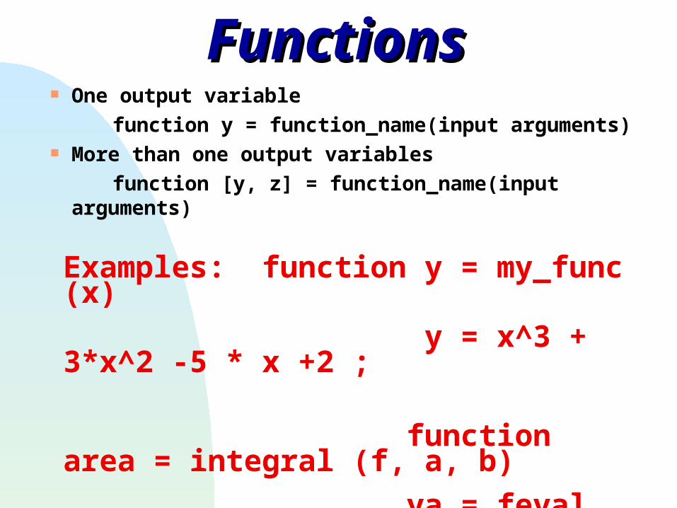
FunctionsFunctions One output variable

function y = function_name(input arguments) More than one output variables

function [y, z] = function_name(input arguments)

Examples: function y = my_func (x)

y = x^3 + 3*x^2 -5 * x +2 ;

function area = integral (f, a, b)

ya = feval (f, a); yb = feval(f, b);

area = (b-a)*(ya+yb)/2;

function t = trap_ex(a, b)t = (b - a) * (a^(-3) + b^(-3)) / 2;

Approximate the integral of f(x) = 1/x3

using basic trapezoid rule

Filename: trap_ex.m

» y = trap_ex (1, 3)y = 1.0370

)(

33

b

a 3 b

1

a

1

2

abdx

x

1y

a b

Script File for IntegralScript File for Integral

1. Save integral (f, a, b) in script file integral.m

2. Save function my_func(x) in script my_func.m

3. Run script file

>> area = integral(‘my_func’, 1, 10)

>> area = integral(‘my_func’, 3, 6)

)b(f)a(f2

abdx)x(f

b

a

area

a b

f(x)

x

feval - evaluate function specified by string

function y = my_func(x)% function 1/x^3y = x.^(-3);

function q = basic_trap(f, a, b)% basic trapezoid rule ya = feval(f, a);yb = feval(f, b);q = (b - a)* (ya + yb)/2;

my_func.m

basic_trap.m

» y = basic_trap ('my_func', 1,3)y = 1.0370

Composite Trapezoid RuleComposite Trapezoid Rule

function I = Trap(f, a, b, n)% find the integral of f using

% composite trapezoid rule

h=(b - a)/n; S = feval(f, a);

for i = 1 : n-1

x(i) = a + h*i;

S = S + 2*feval(f, x(i));

end

S = S + feval(f, b); I =h*S/2;

Filename: comp_trap.m

x

f

a b

Composite Trapezoid RuleComposite Trapezoid Rule» I=comp_trap('my_func',1,3,1)I = 1.0370» I=comp_trap('my_func',1,3,2)I = 0.6435» I=comp_trap('my_func',1,3,4)I = 0.5019» I=comp_trap('my_func',1,3,8)I = 0.4596» I=comp_trap('my_func',1,3,16)I = 0.4483» I=comp_trap('my_func',1,3,100)I = 0.4445» I=comp_trap('my_func',1,3,500)I = 0.4444» I=comp_trap('my_func',1,3,1000)I = 0.4444

one segment

two segments

four segments

eight segments

16 segments

100 segments

500 segments

1000 segments

Function File – Bungee JumperFunction File – Bungee Jumper Create a function file freefallvel.m

function velocity = freefallvel(m,cd,t)

% freefallvel(m,cd,t) computes the free-fall velocity (m/s)

% of an object with second-order drag

% input:

% m = mass (kg)

% cd = second-order drag coefficient (kg/m)

% t = time (sec)

% output:

% velocity = downward velocity (m/s)

g = 9.81; % acceleration of gravity

velocity = sqrt(g*m/cd) * tanh(sqrt(g*cd/m)*t);

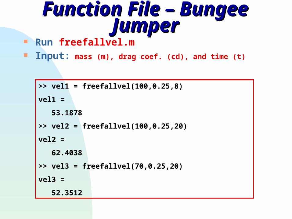
Function File – Bungee JumperFunction File – Bungee Jumper Run freefallvel.m Input: mass (m), drag coef. (cd), and time (t)

>> vel1 = freefallvel(100,0.25,8)

vel1 =

53.1878


vel2 =

62.4038


vel3 =

52.3512

Function FileFunction File To invoke the help comments Type help freefallvel

>> help freefallvel

freefallvel(m,cd,t) computes the free-fall velocity (m/s)

of an object with second-order drag

input:

m = mass (kg)

cd = second-order drag coefficient (kg/m)

t = time (sec)

output:

velocity = downward velocity (m/s)

Function M-FilesFunction M-Files Function M-file can return more than one result Example – mean and standard deviation of a vector

Textbook refers function M-files as simply M-files

function [mean, stdev] = stats(x)

% calculate the mean and standard deviation of a vector x

n = length(x);

mean = sum(x)/n;

stdev = sqrt(sum((x-mean).^2/(n-1)));

>> x=[1.5 3.7 5.4 2.6 0.9 2.8 5.2 4.9 6.3 3.5];

>> [m,s] = stats(x)m = 3.6800s = 1.7662

Data FilesData Files MAT Files -- memory efficient binary format -- preferable for internal use by MATLAB program

ASCII files -- in ASCII characters -- useful if the data is to be shared (imported or

exported to other programs)

MATLAB InputMATLAB Input To read files in

if the file is an ascii table, use “load”

if the file is ascii but not a table, file I/O needs “fopen” and “fclose”

Reading in data from file using fopen depends on type of data (binary or text)

Default data type is “binary”

Save FilesSave Files 8-digit text format (variable list) save <fname> <vlist> - ascii 16-digit text format save <fname> <vlist> - double Delimit elements with tabs save <fname> <vlist> - double - tabs

Example: Vel = [1 3 5; -6 2 -3]

save velocity.dat Vel -ascii

1.0000000e+000 3.0000000e+000 5.0000000e+000 -6.0000000e+000 2.0000000e+000 -3.0000000e+000

Load FilesLoad Files Read velocity into a matrix “velocity.dat”

>> load velocity.dat

>> velocity

velocity = 1 3 5

-6 2 -3

1.0000000e+000 3.0000000e+000 5.0000000e+000 -6.0000000e+000 2.0000000e+000 -3.0000000e+000

Create an ASCII file temperature.dat

read “Time” and “Temperature” from temp.dat >> load temperature.dat >> temperature

% Time Temperature 0.0 75.0 0.5 73.2 1.0 72.6 1.5 74.8 2.0 79.3 2.5 83.2

Load FilesLoad Files

Note: temperature is a 62 matrix

Matlab automatically prints the results of any calculation (unless suppressed by semicolon ;)

Use “disp” to print out text to screen

disp (x.*y)

disp (´Temperature =´)

sprintf - display combination

Make a string to print to the screen

output = sprintf(‘Pi is equal to %f ’, pi)

MATLAB OutputMATLAB Output

Formatted OutputFormatted Outputfprintf (format-string, var, ….)

%[flags] [width] [.precision] type

Examples of “type” fields

%d display in integer format

%e display in lowercase exponential notation

%E display in uppercase exponential notation

%f display in fixed point or decimal notation

%g display using %e or %f, depending on which is shorter

%% display “%”

Numeric Display FormatNumeric Display Format

blank, ,format

00e897931415926535.3decimals 15e longformat

00e1416.3decimals 4eshort format

14.3decimals 2bankformat

89791415926535.3decimals 14longformat

1416.3defaultshortformat

ExampleDisplayCommand MATLAB

x = [5 -2 3 0 1 -2]; format +

x = [+ + + ] (+/ sign only)

fprintf( ) of Scalarfprintf( ) of Scalartemp = 98.6;

fprintf(‘The temperature is %8.1f degrees F.\n’, temp);

The temperature is 98.6 degrees F.

fprintf(‘The temperature is %8.3e degrees F.\n’, temp);

The temperature is 9.860e+001 degrees F.

fprintf(‘The temperature is %08.2f degrees F.\n’, temp);

The temperature is 00098.60 degrees F.

fprintf( ) of fprintf( ) of MatricesMatrices

Score = [1 2 3 4; 75 88 102 93; 99 84 95 105]

Game 1 score: Houston: 75 Dallas: 99




fprintf(‘Game %1.0f score: Houston: %3.0f Dallas: %3.0f \n’,Score)

fprintf control codes

\n Start new line \t Tab

Interactive input FunctionInteractive input Function The input function allows you to prompt the user

for values directly from the command window

Enter either “value” or “stream”

n = input(‘promptstring’)

function [name, sid, phone, email] = register

name = input('Enter your name: ','s');

sid = input('Enter your student ID: ');

phone = input('Enter your Telphone number: ','s');

email = input('Enter your Email address: ','s');

string

value

Interactive input FunctionInteractive input Function>> [name,sid,phone,email] = register

Enter your name: John Doe

Enter your student ID: 12345678

Enter your Telphone number: 987-6543

Enter your Email address: [email protected]

name =

John Doe

sid =

12345678

phone =

987-6543

email =

[email protected]

Interactive M-FileInteractive M-File An interactive M-file for free-falling bungee jumper

Use input and disp functions for input/output

function velocity = freefallinteract

% freefallinteract()

% compute the free-fall velocity of a bungee jumper

% input: interactive from command window

% output: ve;ocity = downward velocity (m/s)

g=9.81; % acceleration of gravity

m = input('Mass (kg): ');

cd = input('Drag coefficient (kg/m): ');

t = input('Time (s): ');

disp(' ')

disp('Velocity (m/s):')

vel = sqrt(g*m/cd)*tanh(sqrt(g*cd/m)*t);

disp([t;vel]’)

Interactive M-FileInteractive M-File>> freefallinteractMass (kg): 68.1Drag coefficient (kg/m): 0.25Time (s): 0:1:20 Velocity (m/s): 0 0 1.0000 9.6939 2.0000 18.7292 3.0000 26.6148 4.0000 33.1118 5.0000 38.2154 6.0000 42.0762 7.0000 44.9145 8.0000 46.9575 9.0000 48.4058 10.0000 49.4214 11.0000 50.1282 12.0000 50.6175 13.0000 50.9550 14.0000 51.1871 15.0000 51.3466 16.0000 51.4560 17.0000 51.5310 18.0000 51.5823 19.0000 51.6175 20.0000 51.6416

CVEN 302-501CVEN 302-501

Homework No. 2Homework No. 2

Chapter 3 Problems 3.1 (25), 3.4 (25)

Due Wed. 09/10/2008 at the Due Wed. 09/10/2008 at the beginning of the periodbeginning of the period

Common Program StructuresCommon Program Structures

Sequence Selection Repetition

Structured ProgrammingStructured ProgrammingModular Design Subroutines (function M-files) called by a main

program

Top-Down Design a systematic development process that begins with

the most general statement of a program’s objective and then successively divides it into more detailed segments

Structured Programming deals with how the actual code is developed so

that it is easy to understand, correct, and modify

The hierarchy of flowcharts dealing with a student’s GPA

•Modular design

•Top-down design

•Structural Programming

Structured ProgrammingStructured Programming

The ideal style of programming is StructuredStructured or ModularModular programming

Break down a large goal into smaller tasks Develop a module for each task A module has a single entrance and exit Modules can be used repeatedly A subroutinesubroutine (function M-file)(function M-file) may contain several

modules Subroutines (Function M-files) called by a main

program

Algorithm DesignAlgorithm Design

The sequence of logical steps required to

perform a specific task (solve a problem)

Each step must be deterministic The process must always end after a finite

number of steps An algorithm cannot be open-ended The algorithm must be general enough to deal

with any contingency

Structured ProgrammingStructured Programming

Sequential paths Sequence – all instructions (statements) are

executed sequentially from top to bottom * A strict sequence is highly limiting

Non-sequential paths Decisions (Selection) – if, else, elseif Loops (Repetition) – for, while, break

Selection Selection ((IFIF)) Statements Statements The most common form of selection

structure is simple if statement The if statement will have a condition

associated with it The condition is typically a logical

expression that must be evaluated as either “true” or “false”

The outcome of the evaluation will determine the next step performed

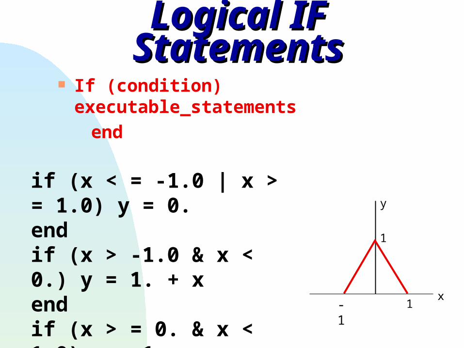
Logical IF StatementsLogical IF Statements If (condition) executable_statements

end

-1 1x

1

y

if (x < = -1.0 | x > = 1.0) y = 0.endif (x > -1.0 & x < 0.) y = 1. + xendif (x > = 0. & x < 1.0) y = 1.- xend

Relation OperatorsRelation Operators

MATLAB == ~= < <= > >= & | ~

Interpretation is equal to is not equal to is less than is less than or equal to is greater than is greater than or equal to and, true if both are true or, true if either one is true not

Logical ConditionsLogical Conditions ~ (not) – logical negation of an expression ~ expression If the expression is true, the result is false.

Conversely, if the expression is false, the result is true.

& (and) – logical conjunction on two expressions

expression1 & expression2

If both expressions are true, the result is true. If either or both expressions are false, the result is false.

| (or) – logical disjunction on two expressions

expression1 | expression2

If either or both expressions are true, the result is true

Logical OperatorsLogical Operators 0 - 1 matrix 0: false ; 1: True

011ans cb | ba

001ans cb & ba

111ans b~a

011ans ba

234c 153b 642a

True Table for Logical OperatorsTrue Table for Logical Operators Order of priority of logical operators

x y ~x x&y x|y

T T F T T

T F F F T

F T T F F

F F T F F

Highest Lowest

Example of a Complex DecisionExample of a Complex Decision

If a=-1, b=2, x=1, and y=‘b’, evaluate

A * b > 0 & b == 2 & x > 7 | ~(y > ‘d’)

1. Expression 1: A*b = -2 > 0 (false)

2. Expression 2: b = 2 (true)

3. Expression 3: x = 1 > 7 (false)

4. Expression 4: ‘b’ > ‘d’ (false)

5. Expression 5: ~(Expression 4) (true)

6. Expression 6: (Expression 1) & (Expression 2) (false)

7. Expression 7: (Expression 6) & (Expression 3) (false)

8. Expression 8: (Expression 7) | (Expression 5) (true)

Complex DecisionComplex Decision A step-by-step evaluation of a complex decision

Nested IF StatementNested IF Statement

if (condition) statement blockelseif (condition) another statement blockelse another statement blockend

Structures can be nested within each other

How to use Nested IFHow to use Nested IF If the condition is true the

statements following the statement block are executed.

If the condition is not true, then the control is transferred to the next

else, elseif, or end statement at the same if level.

Else and ElseifElse and Elseifif temperature > 100

disp(‘Too hot - equipment malfunctioning.’)

elseif temperature > 75

disp(‘Normal operating range.’)

elseif temperature > 60

disp(‘Temperature below desired operating range.’)

else

disp(‘Too Cold - turn off equipment.’)

end

Nested IF StatementsNested IF Statements nested if (if, if else, if elseif)

-1 1x

1

y

if (x < = -1.0)

y = 0.

elseif (x < = 0.)

y = 1. + x

elseif (x < = 1.0)

y = 1. - x

else

y=0.

end

M-file: Evaluate CVEN 302 GradeM-file: Evaluate CVEN 302 Grade function cven302_gradename = input('Enter Student Name: ','s');sid = input('Enter Student ID: ');HW = input('Enter Homework Average (30%): ');Exam1 = input('Enter Exam I score (20%): ');Exam2 = input('Enter Exam II score (20%): ');Final = input('Enter Final Exam score (30%): ');Average= HW*0.3 + Exam1*0.2 + Exam2*0.2 + Final*0.3; fprintf('Your Semester Average is: %6.2f \n',Average)if Average >= 90 Grade = 'A';elseif Average >= 80 Grade = 'B';elseif Average >= 70 Grade = 'C';elseif Average >= 60 Grade = 'D';else Grade = 'F';endfprintf('Your Semester Grade is : '), disp(Grade)

>> cven302_grade

Enter Student Name: Jane Doe

Enter Student ID: 1234567

Enter Homework Average (30%): 96

Enter Exam I score (20%): 88

Enter Exam II score (20%): 92

Enter Final Exam score (30%): 85

Your Semester Average is: 90.30

Your Semester Grade is : A

>> cven302_grade

Enter Student Name: John Doe

Enter Student ID: 9876543

Enter Homework Average (30%): 62

Enter Exam I score (20%): 84

Enter Exam II score (20%): 80

Enter Final Exam score (30%): 91

Your Semester Average is: 78.70

Your Semester Grade is : C

Decisions (Selections)Decisions (Selections) if … elseif if … elseif

StructureStructure

RepetitionRepetition

for i=1:mfor j=1:n

a(i,j)=(i+1)^2*sin(0.2*j*pi);end

end

Do loopsDo loops

For LoopsFor Loopsfor index = start : step : finish statementsend

for k = 1:length(d)

if d(k) < 30

velocity(k) = 0.5 - 0.3*d(k).^2;

else

velocity(k) = 0.6 + 0.2*d(k)-0.01*d(k).^2

end

end

Ends after a specified number

of repetitions

For LoopFor Loopfunction A = for_loop(m,n)

for i = 1:m

for j = 1:n

A(i,j) = 50*exp(-0.2*i)^2*sin(0.1*j*pi);

end

end

>> A = for_loop(8,6)

A =

10.3570 19.7002 27.1150 31.8756 33.5160 31.8756

6.9425 13.2054 18.1757 21.3669 22.4664 21.3669

4.6537 8.8519 12.1836 14.3226 15.0597 14.3226

3.1195 5.9336 8.1669 9.6007 10.0948 9.6007

2.0910 3.9774 5.4744 6.4356 6.7668 6.4356

1.4017 2.6661 3.6696 4.3139 4.5359 4.3139

0.9396 1.7872 2.4598 2.8917 3.0405 2.8917

0.6298 1.1980 1.6489 1.9384 2.0381 1.9384

For LoopFor Loop M-file for computing the factorial n! MATLAB has a built-in function factorial(n) to compute n!

function fout = factor(n)

% factor(n):

% Computes the product of all the integers from 1 to n.

x=1;

for i = 1:n

x = x*i;

end

fout = x;

>> factor(12)

ans =

479001600

>> factor(100)

ans =

9.332621544394410e+157

While LoopsWhile Loops

while condition statementsend

If the statement is true, the statements are executed

If the statement is always true, the loop becomes an “infinite loop”

The “break” statement can be used to terminate the “while” or “for” loop prematurely.

Ends on the basis of a logical condition

While LoopWhile Loop Compute your checking account balancefunction checking

% Compute balance in checking account

Balance = input('Current Checking Account Balance ($) = ');

Deposit = input('Monthly Deposit ($) = ');

Subtract = input('Monthly Subtractions ($) = ');

Month = 0;

while Balance >= 0

Month = Month + 1;

Balance = Balance + Deposit - Subtract;

if Balance >= 0

fprintf('Month %3d Account Balance = %8.2f \n',Month,Balance)

else

fprintf('Month %3d Account Closed \n',Month)

end

end

While LoopWhile Loop>> checking

Current Checking Account Balance ($) = 8527.20

Monthly Deposit ($) = 1025.50

Monthly Subtractions ($) = 1800

Month 1 Account Balance = 7752.70











Month 12 Account Closed

Nesting and IndentationNesting and Indentation Example: Roots of a Quadratic Equation

a

acbbx

cbxax

2

4

02

2

If a=0, b=0, no solution (or trivial sol. c=0)

If a=0, b0, one real root: x=-c/b

If a0, d=b2 4ac 0, two real roots

If a0, d=b2 4ac <0, two complex roots

Nesting and IndentationNesting and Indentationfunction quad = quadroots(a,b,c)% Computes real and complex roots of quadratic equation% a*x^2 + b*x + c = 0% Output: (r1,i1,r2,i2) - real and imaginary parts of the% first and second rootif a == 0 % weird cases if b ~= 0 % single root r1 = -c/b else % trivial solution error('Trivial or No Solution. Try again') end % quadratic formulaelsed = b^2 - 4*a*c; % discriminant if d >= 0 % real roots r1 = (-b + sqrt(d)) / (2*a) r2 = (-b - sqrt(d)) / (2*a) else % complex roots r1 = -b / (2*a) r2 = r1 i1 = sqrt(abs(d)) / (2*a) i2 = -i1 endend

Roots of Quadratic EquationRoots of Quadratic Equation>> quad = quadroots(5,3,-4)

r1 =

0.6434

r2 =

-1.2434

>> quad = quadroots(5,3,4)

r1 =

-0.3000

r2 =

-0.3000

i1 =

0.8426

i2 =

-0.8426

>> quad = quadroots(0,0,5)

??? Error using ==> quadroots

Trivial or No Solution. Try again

(two real roots)

(two complex roots)

(no root)

Passing Functions to M-FilePassing Functions to M-File Use built-in “feval” and “inline” functions to

perform calculations using an arbitrary function

outvar = feval(‘funcname’, arg1, arg2, …)

Funcname = inline(‘expression’, var1, var2, ...)

>> fx=inline('exp(-x)*cos(x)^2*sin(2.*x)')

fx =

Inline function:

fx(x) = exp(-x)*cos(x)^2*sin(2.*x)

>> y = fx(2/3*pi)

y =

-0.0267

No need to store in

separate M-file

Bungee Jumper: Euler’s MethodBungee Jumper: Euler’s Methodfunction [x, y] = Euler(f, tspan, y0, n)% solve y' = f(x,y) with initial condition y(a) = y0% using n steps of Euler's method; step size h = (b-a)/n% tspan = [a, b]a = tspan(1); b = tspan(2); h = (b - a) / n;x = (a+h : h : b);y(1) = y0 + h*feval(f, a, y0);for i = 2 : n y(i) = y(i-1) + h*feval(f, x(i-1), y(i-1));endx = [ a x ];y = [y0 y ];

function f = bungee_f(t,v)

% Solve dv/dt = f for bungee jumper velocity

g = 9.81; m = 68.1; cd = 0.25;

f = g - cd*v^2/m;

Use “feval” for function evaluation

MATLAB M-File: Bungee JumperMATLAB M-File: Bungee Jumper[t,v] = bungee_exact; hold on; % Exact Solution

[t1,v1] = Euler('bungee_f',[0 20],0,10); % Euler method

h1=plot(t1,v1,'g-s');

set(h1,'LineWidth',3,'MarkerSize',10);

[t2,v2] = Euler('bungee_f',[0 20],0,20); %Euler method

h2 = plot(t2,v2,'k:d');


[t3,v3] = Euler('bungee_f',[0 20],0,100); %Euler method

h3 = plot(t3,v3,'mo'); hold off;


h4 = title('Bungee Jumper'); set(h4,'FontSize',20);

h5 = xlabel('Time (s)'); set(h5,'FontSize',20);

h6 = ylabel('Velocity (m/s)'); set(h6,'FontSize',20);

h7 = legend('Exact Solution','\Delta t = 2 s','\Delta t = 1 s‘, '\Delta t = 0.2s',0);

set(h7,'FontSize',20);

Bungee Jumper VelocityBungee Jumper Velocity

M-File: Bichromatic WavesM-File: Bichromatic Waves Filename waves.m (script file)

% Plot Bi-chromatic Wave Profilea1 = 1; a2 = 1.5; c1 = 2.0; c2 = 1.8;time = 0:0.1:100;wave1 = a1 * sin(c1*time);wave2 = a2 * sin(c2*time) + a1;wave3 = wave1 + wave2;plot(time,wave1,time,wave2,time,wave3)axis([0 100 -2 4]);xlabel ('time'); ylabel ('wave elevation');title ('Bi-chromatic Wave Profile')text(42,-1.2, 'wave 1')text(42, 2.7, 'wave 2')text(59, 3.6, 'waves 1+2')

MATLAB SubplotsMATLAB Subplots Filename waves2.m (script file)

% Plot Bi-chromatic Wave Profile% Display the results in three subplotsclf % clear the graphics windowa1 = 1; a2 = 1.5; c1 = 2.0; c2 = 1.8;time = 0:0.1:100;wave1 = a1 * sin(c1*time);wave2 = a2 * sin(c2*time);wave3 = wave1 + wave2;subplot(3,1,1) % top figureplot(time,wave1,'m'); axis([0 100 -3 3]); ylabel('wave 1');subplot(3,1,2) % middle figureplot(time,wave2,'g'); axis([0 100 -3 3]); ylabel('wave 2');subplot(3,1,3) % bottom figureplot(time,wave3,'r'); axis([0 100 -3 3]);xlabel(’time'); ylabel('waves 1&2');

subplot ( m, n, p ) --

breaks the figure window into m by n small figures, select the p-th figure for the current plot

» figure (3)» subplot (3, 2, 1)» plot (t,wv1)» subplot (3, 2, 2)» plot (t,wv2)» subplot (3, 2, 4)» plot (t, wv1+wv2)» subplot (3, 2, 6)» plot (t, wv1-wv2)

MATLAB SubplotsMATLAB Subplots

1 2

3 4

5 6

» x=0:0.1:10; y1=sin(pi*x); y2=sin(0.5*pi*x); y3=y1+y2;» z1=cos(pi*x); z2=cos(0.5*pi*x); z3=z1-z2;» subplot(3,2,1); H1=plot(x,y1,'b'); set(H1,'LineWidth',2);» subplot(3,2,2); H2=plot(x,z1,'b'); set(H2,'LineWidth',2);» subplot(3,2,3); H3=plot(x,y2,'m'); set(H3,'LineWidth',2);» subplot(3,2,4); H4=plot(x,z2,'m'); set(H4,'LineWidth',2);» subplot(3,2,5); H5=plot(x,y3,'r'); set(H5,'LineWidth',2);» subplot(3,2,6); H6=plot(x,z3,'r'); set(H6,'LineWidth',2);

Subplot (m,n,p)

Multiple plots

CVEN 302-501CVEN 302-501

Homework No. 3Homework No. 3

Chapter 3 Problems 3.6 (35), 3.9 (35)

Due Mon 09/15/08 at the beginning Due Mon 09/15/08 at the beginning of the periodof the period

chapter 3 programming with matlab. newton’s second law euler’s method to obtain good...

Documents

function file function

script file slide

word function function

function area

script file integral

function t

script file area

script files script