Chapter 3 - Part 1

AERO-423

Orbit Transfer

3-2

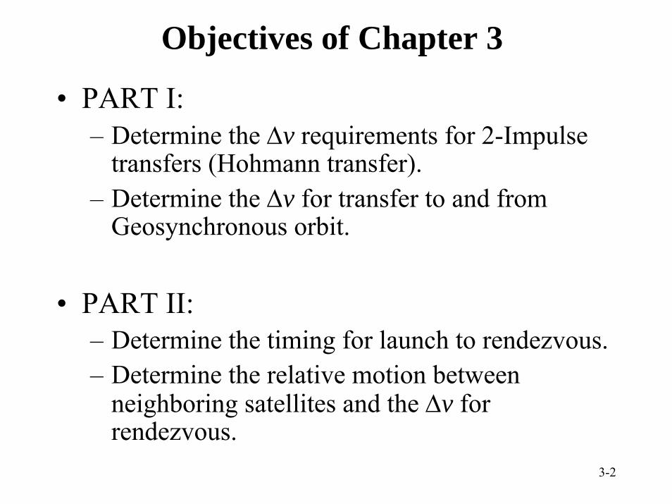
Objectives of Chapter 3

• PART I:– Determine the Δv requirements for 2-Impulse

transfers (Hohmann transfer).– Determine the Δv for transfer to and from

Geosynchronous orbit.

• PART II:– Determine the timing for launch to rendezvous.– Determine the relative motion between

neighboring satellites and the Δv for rendezvous.

3-3

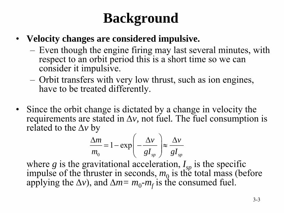
• Velocity changes are considered impulsive.– Even though the engine firing may last several minutes, with

respect to an orbit period this is a short time so we can consider it impulsive.

– Orbit transfers with very low thrust, such as ion engines, have to be treated differently.

• Since the orbit change is dictated by a change in velocity the requirements are stated in Δv, not fuel. The fuel consumption is related to the Δv by

where g is the gravitational acceleration, Isp is the specific impulse of the thruster in seconds, m0 is the total mass (before applying the Δv), and Δm= m0-mf is the consumed fuel.

Background

0

1 expsp sp

m v vm gI gI

⎛ ⎞Δ Δ Δ= − − ≈⎜ ⎟⎜ ⎟

⎝ ⎠

3-4

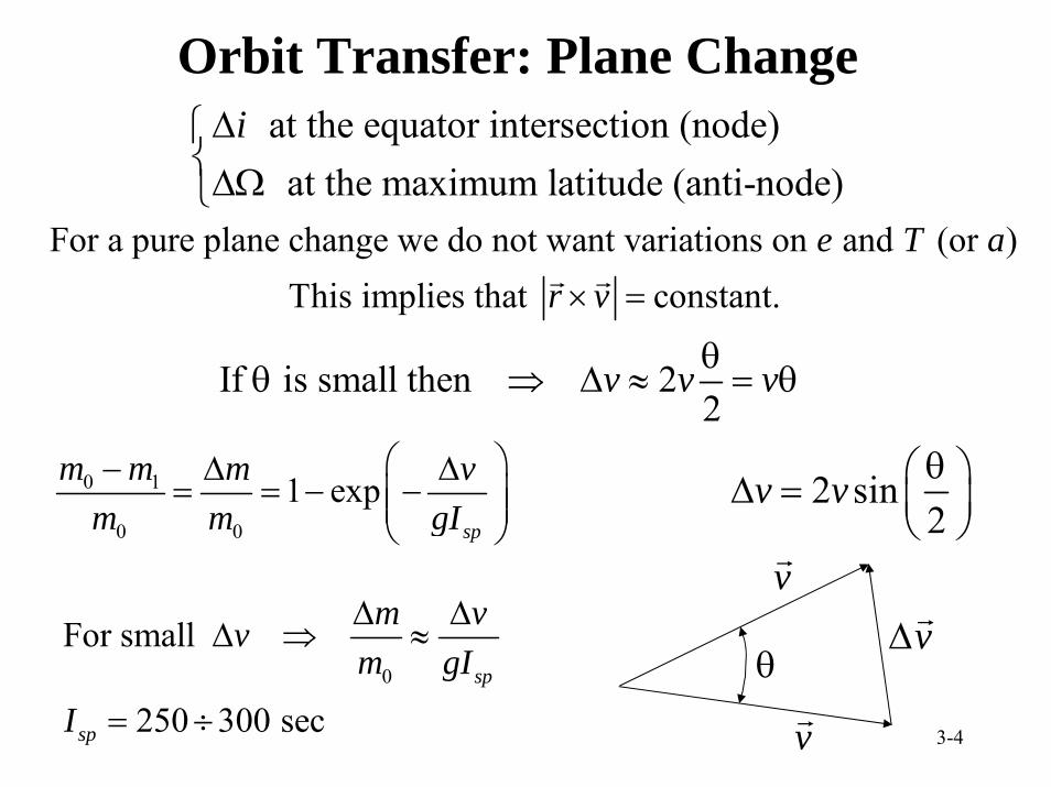
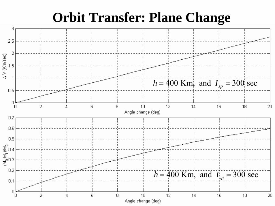
Orbit Transfer: Plane Change

If is small then 22

v v vθθ ⇒ Δ ≈ = θ

2 sin2

v v θ⎛ ⎞Δ = ⎜ ⎟⎝ ⎠

0 1

0 0

1 expsp

m m m vm m gI

⎛ ⎞− Δ Δ= = − −⎜ ⎟⎜ ⎟

⎝ ⎠

v

v

θ Δ

v 0

For small

250 300 secsp

sp

m vvm gI

I

Δ ΔΔ ⇒ ≈

= ÷

at the equator intersection (node) at the maximum latitude (anti-node)

iΔ⎧⎨ΔΩ⎩

For a pure plane change we do not want variations on and (or )This implies that constant.

e T ar v× =

3-5

Orbit Transfer: Plane Change

400 Km, and 300 secsph I= =

400 Km, and 300 secsph I= =

3-6

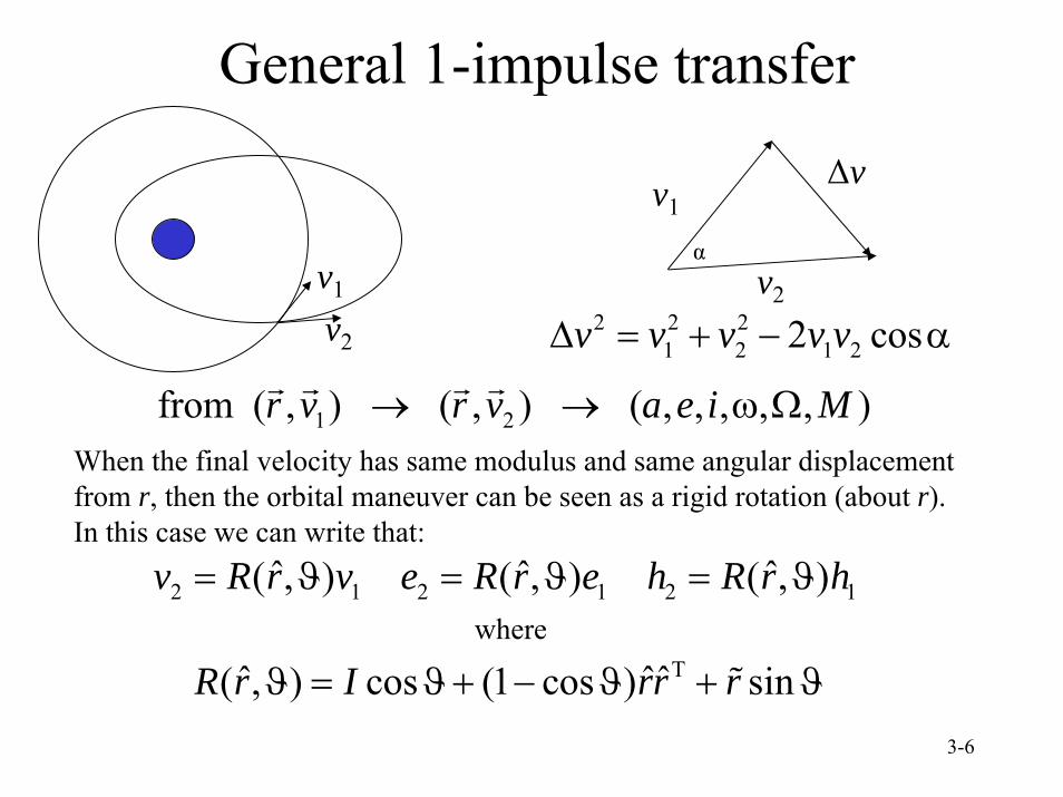
General 1-impulse transfer

v1

v2

Δv

v2

v12 2 2

1 2 1 22 cosv v v v vΔ = + − α

1 2from ( , ) ( , ) ( , , , , , )r v r v a e i M→ → ω Ω

α

When the final velocity has same modulus and same angular displacementfrom r, then the orbital maneuver can be seen as a rigid rotation (about r).In this case we can write that:

2 1 2 1 2 1ˆ ˆ ˆ( , ) ( , ) ( , )v R r v e R r e h R r h= ϑ = ϑ = ϑ

Tˆ ˆˆ( , ) cos (1 cos ) sinR r I rr rϑ = ϑ+ − ϑ + ϑwhere

3-7

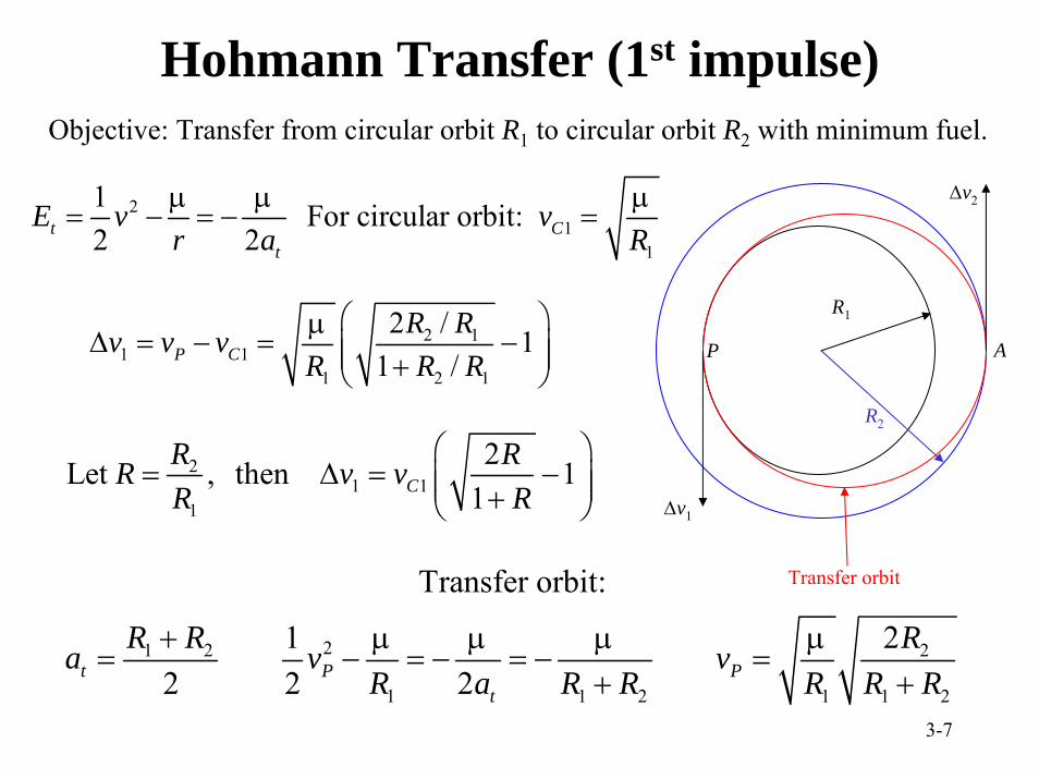
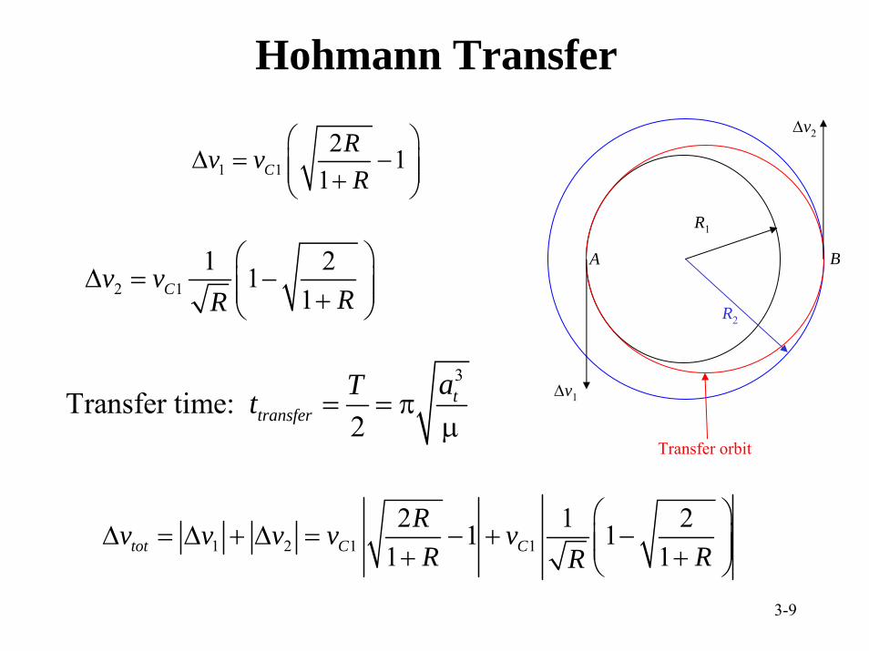
Hohmann Transfer (1st impulse)Objective: Transfer from circular orbit R1 to circular orbit R2 with minimum fuel.

R2

R1

P A

Δv1

Δv2

Transfer orbit

21 2 2

1 1 2 1 1 2

Transfer orbit:

212 2 2t P P

t

R R Ra v vR a R R R R R

+ μ μ μ μ= − = − = − =

+ +

21

1

1 For circular orbit: 2 2t C

t

E v vr a Rμ μ μ

= − = − =

2 11 1

1 2 1

2 / 11 /P C

R Rv v vR R R

⎛ ⎞μΔ = − = −⎜ ⎟⎜ ⎟+⎝ ⎠

21 1

1

2Let , then 11C

R RR v vR R

⎛ ⎞= Δ = −⎜ ⎟⎜ ⎟+⎝ ⎠

3-8

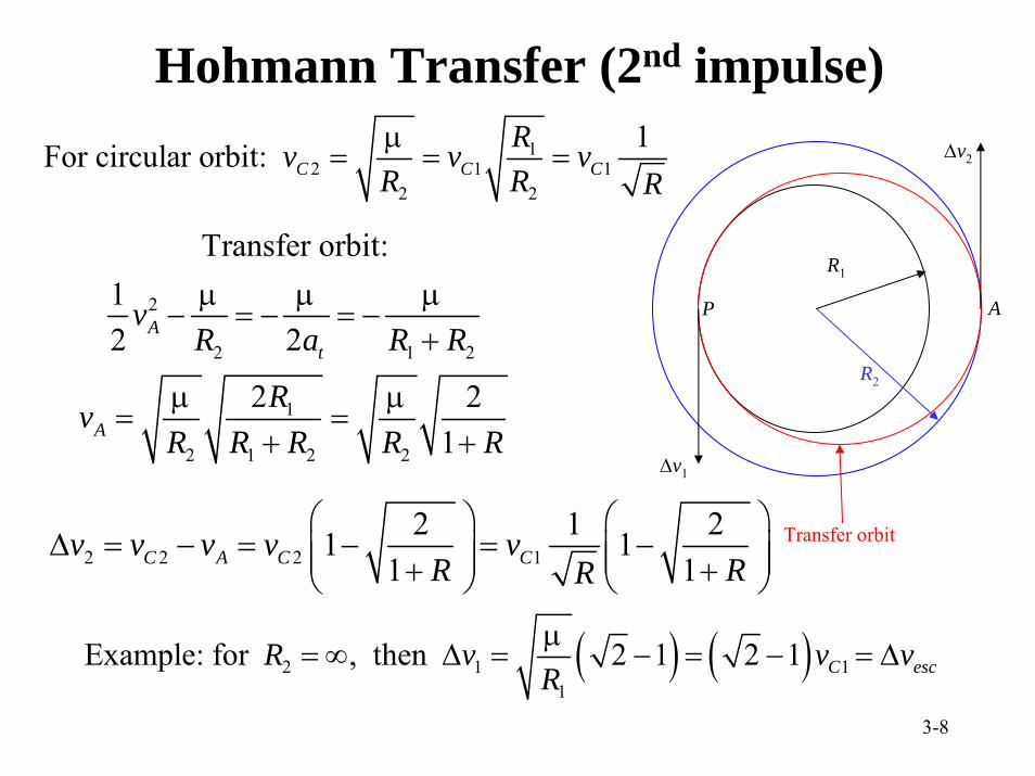
Hohmann Transfer (2nd impulse)1

2 1 12 2

1For circular orbit: C C CRv v v

R R Rμ

= = =

( ) ( )2 1 11

Example: for , then 2 1 2 1 C escR v v vRμ

= ∞ Δ = − = − = Δ

R2

R1

P A

Δv1

Δv2

Transfer orbit

2

2 1 2

1

2 1 2 2

Transfer orbit:12 2

2 21

At

A

vR a R R

RvR R R R R

μ μ μ− = − = −

+

μ μ= =

+ +

2 2 2 12 1 21 1

1 1C A C Cv v v v vR RR

⎛ ⎞ ⎛ ⎞Δ = − = − = −⎜ ⎟ ⎜ ⎟⎜ ⎟ ⎜ ⎟+ +⎝ ⎠ ⎝ ⎠

3-9

Hohmann Transfer

R2

R1

A B

Δv1

Δv2

Transfer orbit

2 11 21

1Cv vRR

⎛ ⎞Δ = −⎜ ⎟⎜ ⎟+⎝ ⎠

1 12 1

1CRv vR

⎛ ⎞Δ = −⎜ ⎟⎜ ⎟+⎝ ⎠

1 2 1 12 1 21 1

1 1tot C CRv v v v vR RR

⎛ ⎞Δ = Δ + Δ = − + −⎜ ⎟⎜ ⎟+ +⎝ ⎠

3

Transfer time: 2

ttransfer

aTt = = πμ

3-10

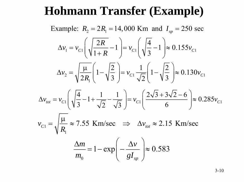
Hohmann Transfer (Example)

1 1 14 1 1 2 3 3 2 61 0.2853 62 3tot C C Cv v v v

⎛ ⎞ ⎛ ⎞+ −Δ = − + − = ≈⎜ ⎟ ⎜ ⎟⎜ ⎟ ⎜ ⎟

⎝ ⎠ ⎝ ⎠

0

1 exp 0.583sp

m vm gI

⎛ ⎞Δ Δ= − − ≈⎜ ⎟⎜ ⎟

⎝ ⎠

2 1

1 1 1 1

Example: 2 14,000 Km and 250 sec

2 41 1 0.1551 3

sp

C C C

R R I

Rv v v vR

= = =

⎛ ⎞ ⎛ ⎞Δ = − = − ≈⎜ ⎟ ⎜ ⎟⎜ ⎟ ⎜ ⎟+⎝ ⎠ ⎝ ⎠

2 1 11

2 1 21 1 0.1302 3 32C Cv v v

R⎛ ⎞ ⎛ ⎞μ

Δ = − = − ≈⎜ ⎟ ⎜ ⎟⎜ ⎟ ⎜ ⎟⎝ ⎠ ⎝ ⎠

11

7.55 Km/sec 2.15 Km/secC totv vRμ

= ≈ ⇒ Δ ≈

3-11

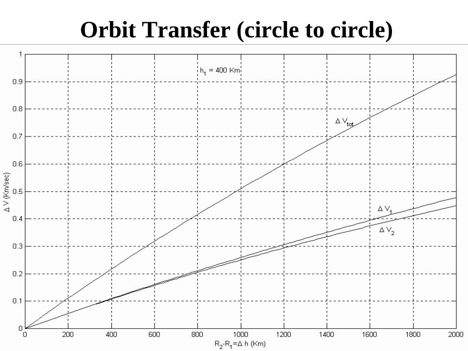
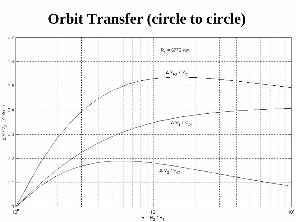
Orbit Transfer (circle to circle)

3-12

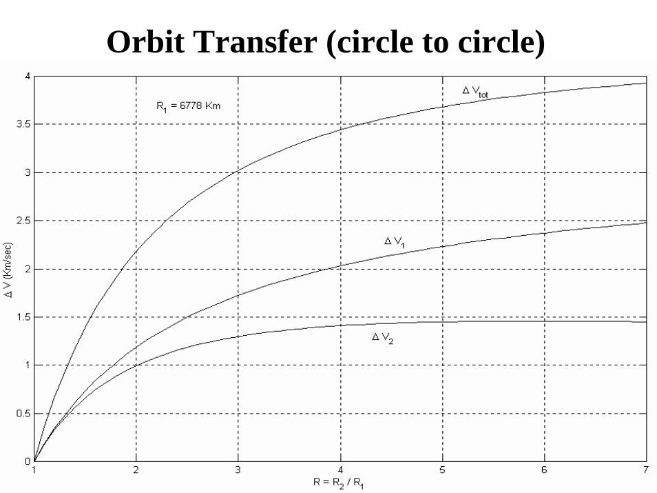
Orbit Transfer (circle to circle)

3-13

Orbit Transfer (circle to circle)

3-14

1

2

3

4

5

6

7

0 0,05 0,1 0,15 0,2 0,25 0,3 0,35 0,4 0,45 0,5

Δv/vc1

R =

R2/R

1

0

5

10

15

20

25

30

35

Δi -

deg

Hohmann

R1 = 6778 km

Plane change

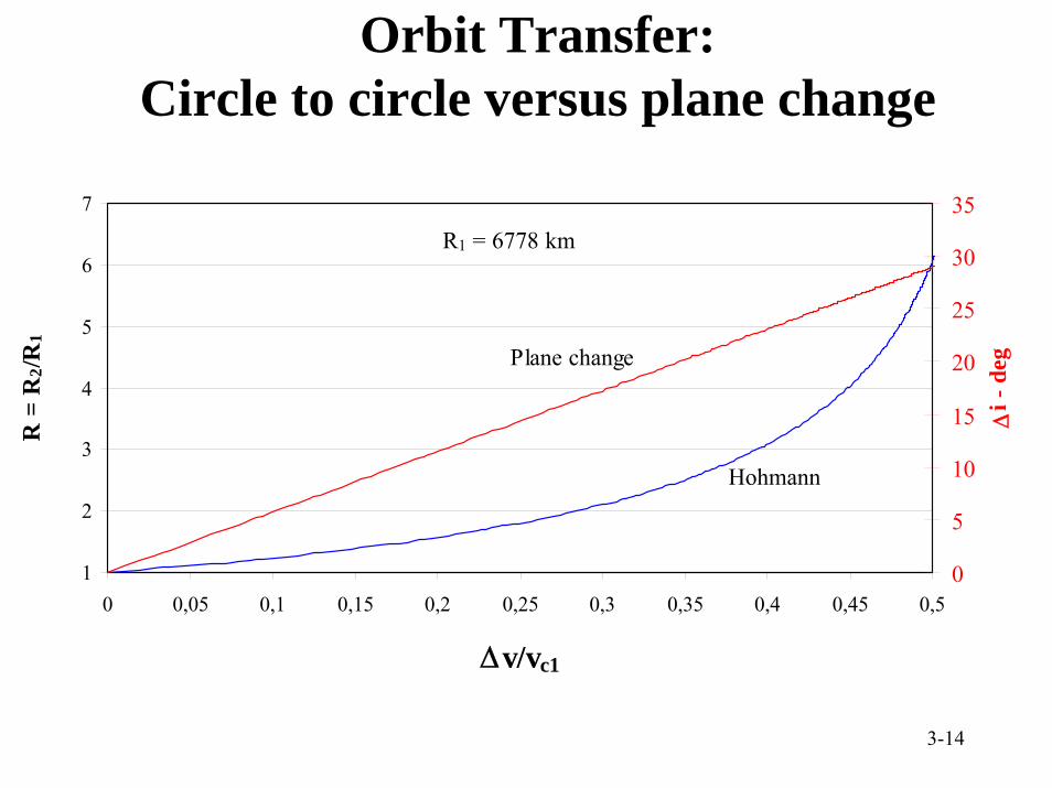
Orbit Transfer:Circle to circle versus plane change

3-15

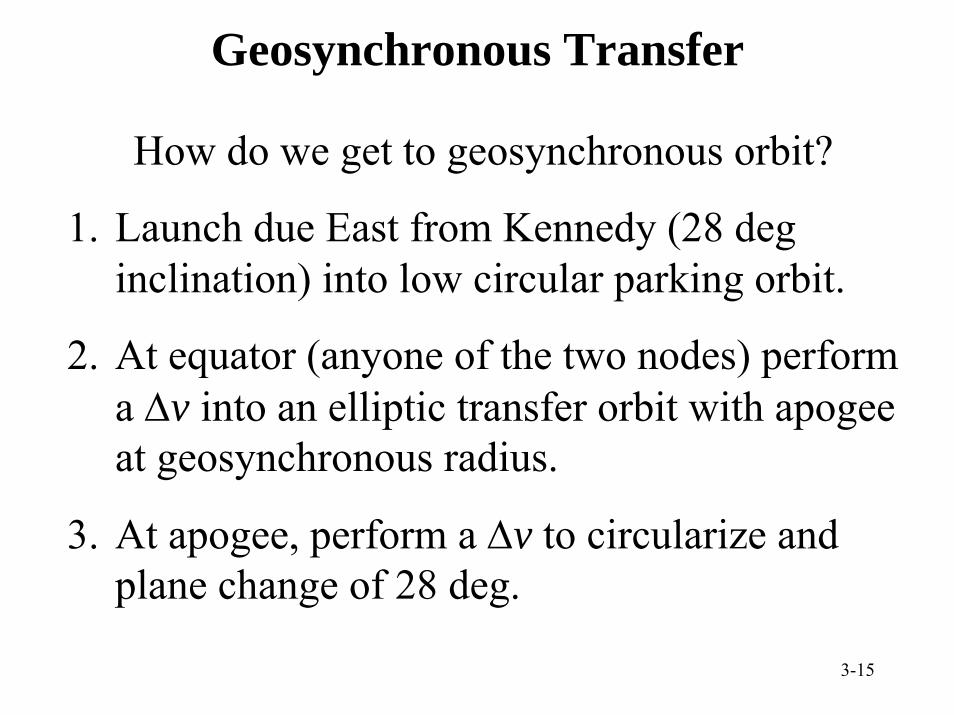
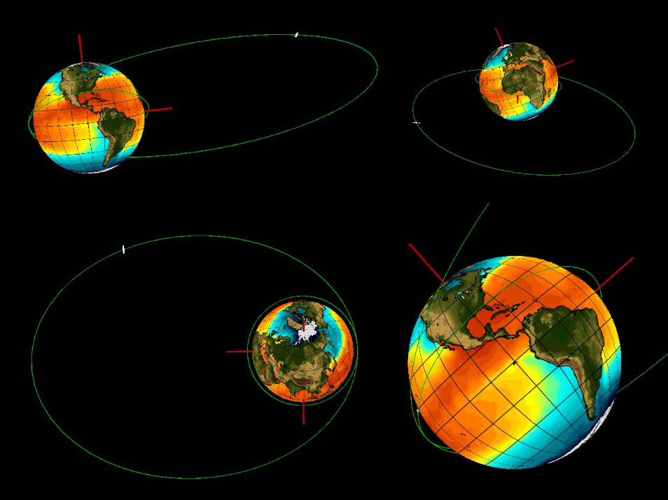
Geosynchronous Transfer

How do we get to geosynchronous orbit?

1. Launch due East from Kennedy (28 deg inclination) into low circular parking orbit.

2. At equator (anyone of the two nodes) perform a Δv into an elliptic transfer orbit with apogee at geosynchronous radius.

3. At apogee, perform a Δv to circularize and plane change of 28 deg.

3-16

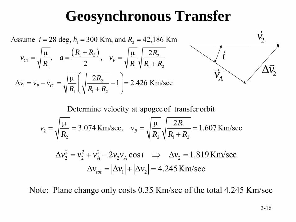
Geosynchronous Transfer

( )1 2

1 2 21

1 1 1 2

21 1

1 1 2

Assume 28 deg, 300 Km, and 42,186 Km

2, ,2

2 1 2.426 Km/sec

C P

P C

i h R

R R Rv a vR R R R

Rv v vR R R

= = =

+μ μ= = =

+

⎛ ⎞μΔ = − = − =⎜ ⎟⎜ ⎟+⎝ ⎠

12

2 2 1 2

Determine velocity at apogeeof transfer orbit

23.074 Km/sec, 1.607 Km/secBRv v

R R R Rμ μ

= = = =+

2 2 22 2 2 2

1 2

2 cos 1.819 Km/sec4.245Km/sec

A A

tot

v v v v v i vv v v

Δ = + − ⇒ Δ =

Δ = Δ + Δ =

2v

2vΔ

Note: Plane change only costs 0.35 Km/sec of the total 4.245 Km/sec

i

Av

3-17