chapter 3: observations: ocean - david appell ocean.pdfzero order draft chapter 3 ipcc wgi fifth...
TRANSCRIPT

Zero Order Draft Chapter 3 IPCC WGI Fifth Assessment Report
Do Not Cite, Quote or Distribute 3-1 Total pages: 70
1 Chapter 3: Observations: Ocean 2
3 Coordinating Lead Authors: Monika Rhein (Germany), Stephen R. Rintoul (Australia) 4 5 Lead Authors: Shigeru Aoki (Japan), Edmo Campos (Brazil), Don Chambers (USA), Richard Feely (USA), 6 Sergey Gulev (Russia), Gregory C. Johnson (USA), Simon Josey (UK), Andrey Kostianoy (Russia), Cecilie 7 Mauritzen (Norway), Dean Roemmich (USA), Lynne Talley (USA), Fan Wang (China) 8 9 Contributing Authors: Michio Aoyama, Molly Baringer, Nick Bates, Timothy Boyer, Robert Byrne, Stuart 10 Cunningham, Thierry Delcroix, John Dore, Melchor González-Dávila, Nicolas Gruber, Mark Hemer, David 11 Hydes, Stanley Jacobs, Torsten Kanzow, David Karl, Alexander Kazmin, Samar Khatiwala, Joan Kleypas, 12 Kitack Lee, Calvin Mordy, Jon Olafsson, James Orr, Igor Polyakov, Bo Qiu, Anastasia Romanou, Raymond 13 Schmitt, Koji Shimada, Lothar Stramma, Toshio Suga, Taro Takahashi, Toste Tanhua, Hans von Storch, 14 Richard Wanninkhof, Susan Wijffels, Phil Woodworth, Lisan Yu 15 16 Review Editors: Howard Freeland (Canada), Yukihiro Nojiri (Japan), Ilana Wainer (Brazil) 17 18 Date of Draft: 15 April 2011 19 20 Notes: TSU Compiled Version 21 22 23 Table of Contents 24 25 Executive Summary..........................................................................................................................................326 3.1 Introduction ..............................................................................................................................................527 3.2 Changes in Ocean Temperature and Heat Content ..............................................................................528
3.2.1 Background: Instruments and Sampling.........................................................................................529 3.2.2 Upper Ocean Temperature Changes ..............................................................................................630 3.2.3 Upper Ocean Heat Content Variability ..........................................................................................731 3.2.4 Deep Ocean Heat Content Variability ............................................................................................832
Box 3.1: Change in Global Energy Inventory ................................................................................................833 3.3 Changes in the Salinity and Freshwater Budget ...................................................................................934
3.3.1 Introduction.....................................................................................................................................935 3.3.2 Global to Basin-Scale Trends .......................................................................................................1036 3.3.3 Regional Changes in Salinity ........................................................................................................1137 3.3.4 Evidence for Change of the Global Water Cycle from Salinity ....................................................1238
3.4 Changes in Ocean Surface Fluxes .........................................................................................................1339 3.4.1 Introduction...................................................................................................................................1340 3.4.2 Air-Sea Heat Flux .........................................................................................................................1341 3.4.3 Ocean Surface Precipitation and Freshwater Flux ......................................................................1542 3.4.4 Wind Stress....................................................................................................................................1543 3.4.5 Conclusions...................................................................................................................................1644
3.5 Changes in Water Mass Properties and Ventilation ...........................................................................1645 3.6 Evidence for Change in Ocean Circulation..........................................................................................1746
3.6.1 Observing Ocean Circulation Variability.....................................................................................1747 3.6.2 Wind-Driven Circulation Variability in the Pacific Ocean ..........................................................1848 3.6.3 The Atlantic Meridional Overturning Circulation (AMOC).........................................................1949 3.6.4 Water Exchange Between Ocean Basins ......................................................................................2050 3.6.5 Conclusion ....................................................................................................................................2151
3.7 Sea Level Change, Ocean Waves and Storm Surges...........................................................................2152 3.7.1 Observations of Long-Term Trends and Patterns in Sea Level ....................................................2153 3.7.2 Observations of Decadal Variations in Trends and Accelerations...............................................2354 3.7.3 Measurements of Components of Sea Level Change ....................................................................2355 3.7.4 Extreme Sea Level and Storm Surges ...........................................................................................2456 3.7.5 Changes in Surface Waves ............................................................................................................2557

Zero Order Draft Chapter 3 IPCC WGI Fifth Assessment Report
Do Not Cite, Quote or Distribute 3-2 Total pages: 70
3.8 Ocean Biogeochemical Changes, Including Anthropogenic Ocean Acidification ............................261 3.8.1 Ocean Carbon ...............................................................................................................................262 3.8.2 Anthropogenic Ocean Acidification..............................................................................................283
Box 3.2: Ocean Acidification .........................................................................................................................284 3.8.3 Oxygen ..........................................................................................................................................315 3.8.4 Regional and Long-Term Trends in Nutrient Distributions in the Oceans...................................326
3.9 Synthesis ..................................................................................................................................................327 FAQ 3.1: Is the Ocean Warming?.................................................................................................................338 FAQ 3.2: How Does Anthropogenic Ocean Acidification Relate to Climate Change? ............................359 FAQ 3.3: Is There Evidence for Changes in the Earth’s Water Cycle?....................................................3510 References........................................................................................................................................................3711 Figures .............................................................................................................................................................48 12 13
14

Zero Order Draft Chapter 3 IPCC WGI Fifth Assessment Report
Do Not Cite, Quote or Distribute 3-3 Total pages: 70
Executive Summary 1 2 It is virtually certain that the oceans have warmed over the last four decades. Instrumental biases in historical 3 upper ocean temperature measurements have been identified and largely removed, resulting in a dramatic 4 reduction in the interdecadal variability of global annual average time series of temperature and upper ocean 5 heat content, thus providing stronger evidence of ocean warming than in AR4. Globally averaged ocean 6 temperature anomalies as a function of depth and time reveal warming to at least 1500 m depth over the 7 relatively well-sampled last 43 years. The strongest warming is found near the sea surface (>0.1oC per 8 decade in the upper 75 m), decreasing to about 0.017oC per decade at 700 m. The surface intensification of 9 the warming signal has increased the thermal stratification of the upper ocean by about 4% (between 0 and 10 200 m depth) over the 43-year record. 11 12 Ocean warming accounts for more than 93% of the increase in heat energy stored by the Earth system over 13 the last 50 years. Three different estimates reveal an increase in globally-averaged upper ocean heat content 14 from the 1950s to the present. Although the rates of energy gain differ depending on the strategy used to map 15 changes in temperature in data-poor regions (from 77 to 170 TW in the relatively well-sampled period 1970–16 2003), the three estimates are all positive and there is high agreement and robust evidence that upper ocean 17 heat content has increased. 18 19 Analyses of ocean salinity changes over the last fifty years reveal large, robust and spatially coherent trends 20 in the upper 2000 m. Surface salinity has increased in evaporation-dominated subtropical gyres and 21 freshened in precipitation-dominated regions, and basin-to-basin contrasts have increased, consistent with an 22 enhanced hydrological cycle. Significant trends have been observed in subsurface salinity, reflecting both 23 changes in freshwater flux at the sea surface and poleward migration of isopycnal outcrops caused by ocean 24 warming. 25 26 The temperature and salinity of major water masses have changed in recent decades, in line with changes in 27 surface waters in the formation regions. Surface waters have warmed in each basin and the thermocline 28 waters renewed by surface waters sinking in the tropics and subtropics have generally become warmer, 29 saltier and lighter. Intermediate waters formed at higher latitude have become fresher. Widespread warming 30 has been observed in abyssal waters supplied by Antarctic Bottom Water, which has also freshened in the 31 Indian and Pacific. The deep water masses of the North Atlantic vary strongly on interannual to multidecadal 32 time-scales and no significant trend has been detected. 33 34 Direct observations of ocean circulation are generally of short duration, of limited spatial extent and 35 dominated by energetic variability on time-scales from years to decades. As a consequence, there is no clear 36 evidence of trends in ocean circulation. Subsequent to the AR4 report, progress has been made developing a 37 coordinated observing system to measure the Atlantic meridional overturning circulation (e.g., the 38 RAPID/MOCHA array at 26°N). The direct time series are either too short to estimate trends or measure 39 only one component of the flow. Several indirect methods are commonly used to quantify changes in ocean 40 circulation. A wide variety of these estimates in the North Atlantic agree that AMOC transport varies by 2–3 41 Sv on interannual to interdecadal time scales. There is low agreement and limited evidence of a long-term 42 trend in the AMOC volume transport in the last 50 years despite the changes in T/S characteristics and 43 formation rates of the key deep water masses of the AMOC. 44 45 Variability observed in ocean currents is largely consistent with changes in the wind-driven circulation. 46 Changes in wind forcing, in turn, are dominated by the major climate modes of climate variability, including 47 the North Atlantic Oscillation, ENSO and the Pacific Decadal Oscillation. 48 49 An increase in global mean net heat flux into the ocean of <1 W m-2 is sufficient to account for the observed 50 ocean heat content changes. This signal is too small to detect in surface flux data sets, whose uncertainties 51 are typically an order of magnitude larger than this. Similarly, it is not yet possible to establish whether there 52 is a significant trend in the freshwater flux over the past 50 years from surface flux estimates. Wind stress 53 has increased over the past 30 years in the Southern Ocean, likely as a result of ozone loss at high southern 54 latitudes, while there is no evidence for a trend in global mean wind stress. 55 56

Zero Order Draft Chapter 3 IPCC WGI Fifth Assessment Report
Do Not Cite, Quote or Distribute 3-4 Total pages: 70
Recent estimates of global mean sea level rates have not changed significantly since AR4; the rate of 20th 1 century mean sea level rise is 1.7 ± 0.5 mm yr-1. Global mean sea level rates since 1993 continue to be 2 significantly higher than the rates before 1990. The 17-year satellite altimeter record estimate is 3.3 ± 0.4 3 mm yr-1. Tide gauge measurements give a statistically consistent result (3.2 ± 0.5 mm yr-1) over the same 4 period, so there is high confidence that this change in observed sea level rate is real and not an artefact of the 5 different sampling or instruments. The overall pattern of sea level change from 1993 to 2010 is similar to the 6 pattern from 1993 to 2003 discussed in AR4 and is still driven mainly by redistribution of heat associated 7 with changes in the circulation. The warming of the upper ocean from 1961 to 2003 caused a mean 8 thermosteric rate of 0.5 ± 0.1 mm yr-1 (1 standard error), which is 40% higher than previous assessments that 9 were affected by instrumental biases mentioned above. The warming trend of the deep southern and global 10 abyssal ocean centred on 1992–2005 has contributed 0.05 ± 0.02 mm yr-1 (95% confidence) to sea level rise. 11 The mass component of mean sea level rates since 2003 was estimated to range from 1 to 2 mm yr-1, with the 12 most recent estimate being 1.3 ± 0.6 mm yr-1 (90% confidence level). The uncertainty is dominated by 13 uncertainty in the global isostatic adjustment correction required for satellite gravity measurements. 14 Increases in mean sea level are likely responsible for the observed increase in extreme sea level events and 15 storm surges. 16 17 It is likely that surface wave height has increased over much of the Northern Hemisphere oceans since 1900 18 with an acceleration from 1950s onwards. In the Southern Oceans south of 45°S this tendency holds over the 19 last two decades. It is also very likely that extreme waves have grown over the last 60 years. 20 21 The biogeochemical state of the ocean has changed. Three independent calculations of the inventory of 22 anthropogenic carbon dioxide (Cant) agree within the uncertainties of each approach (±25 PgC) and provide 23 high confidence that the ocean inventory of Cant has increased, from 114 ± 22 PgC in 1994 to 140 ± 25 PgC 24 in 2008. The marginal seas contribute an additional 6% of the global inventory. Regional observations of Cant 25 inventory changes are in broad agreement with the expected change resulting from the increase in 26 atmospheric CO2 concentrations and change in atmospheric O2/N2 ratios. 27 28 The uptake of CO2 by the ocean has resulted in a gradual acidification of seawater. Long time series from 29 several ocean sites show declines in pH in the mixed layer between -0.0005 and -0.0018 yr-1, consistent with 30 results from repeat pH measurements along hydrographic transects. It is virtually certain that the pH decline 31 in the surface ocean is solely attributable to the uptake of anthropogenic CO2. In the ocean interior, pH can 32 also be modified by natural physical and biological processes over decadal time scales. 33 34 Dissolved oxygen in the oceanic thermocline decreased globally in the last 20 to 50 years at a rate of 3–5 35 µmol kg-1 per decade with strong regional variations. This long-term deoxygenation is consistent with a 36 reduction in ventilation of the thermocline caused by warming-induced increases in stratification and with 37 the fact that warmer water can hold less oxygen. 38 39 The observed changes in global ocean heat content, salinity, water masses, sea level and biogeochemistry are 40 consistent with changes in the surface ocean (warming, changes in salinity, and uptake of Cant) and their 41 transfer into the interior ocean by known physical, chemical and biological processes. The consistency 42 between the patterns of change revealed in unrelated parameters, using a variety of independent approaches, 43 gives high confidence that the ocean state has changed in the last fifty years. 44
45

Zero Order Draft Chapter 3 IPCC WGI Fifth Assessment Report
Do Not Cite, Quote or Distribute 3-5 Total pages: 70
1 3.1 Introduction 2 3 The oceans influence climate by storing and transporting vast quantities of heat, freshwater, and carbon. The 4 ocean has a large thermal inertia, both because of the large heat capacity of sea water relative to air and 5 because ocean circulation connects the surface and interior ocean. More than three quarters of the flows of 6 freshwater associated with the global water cycle take place over the oceans, through evaporation and 7 precipitation. The ocean contains roughly 50–60 times more carbon than the atmosphere and is at present 8 absorbing about 25% of human emissions, acting to slow the rate of climate change. It further slows the rate 9 of climate change by taking up large amounts of heat. The ocean is also capable of relatively rapid change, 10 with the potential for climate feedbacks. The evolution of climate on time-scales from weeks to millennia is 11 therefore closely linked to the ocean. 12 13 The large inertia of the oceans means that they naturally integrate over short-term variability and often 14 provide a clearer signal of longer-term change. Observations of ocean change therefore provide a means to 15 track the evolution of climate change. Such observations also provide a rigorous and relevant test for climate 16 models. For example, the climate sensitivity of a climate model is a strong function of ocean heat storage. 17 18 Documenting and understanding change in the ocean is a challenge because of the paucity of long-term 19 measurements of the global ocean. However, significant progress has been made since AR4. The Argo array 20 of profiling floats is now providing year-round measurements of temperature and salinity in the upper 2000 21 m for the first time. The satellite altimetry record is now approaching twenty years in length. Longer 22 continuous time series of important components of the meridional overturning circulation begin to emerge, 23 and one observational array to measure the Atlantic overturning circulation is in place since 2004. While 24 these recent data sets do not solve the problem of a lack of historical data, by documenting the seasonal and 25 interannual variability they help isolate longer-term trends in the incomplete observational record. 26 Significant progress has also been made in removing biases and errors in the historical measurements. The 27 spatial and temporal coverage of biogeochemical measurements in the ocean has expanded. As a result of 28 these advances, there is now stronger evidence for change in the ocean and our understanding of the causes 29 of ocean change is improved. 30 31 This chapter summarizes the observational evidence of change in the ocean, with an emphasis on basin- and 32 global-scale changes relevant to climate. 33 34 3.2 Changes in Ocean Temperature and Heat Content 35 36 [PLACEHOLDER FOR FIRST ORDER DRAFT] 37 38 3.2.1 Background: Instruments and Sampling 39 40 The oceans have absorbed much of the build-up of energy in Earth’s climate system over recent decades. 41 Although temperature is the best measured subsurface ocean parameter, these measurements have been made 42 by a variety of instruments with different accuracies, sampling depths, and precision. Both the mix of 43 instruments and the overall sampling patterns have evolved in time and space (Boyer et al., 2009), 44 complicating efforts to determine and interpret long-term change. Since AR4 the significant impact of 45 measurement biases in some of these instruments (the XBT and MBT) on estimates of ocean temperature 46 changes and upper ocean heat content anomalies (hereafter UOHCA) has been recognized (Gouretski and 47 Koltermann, 2007). Careful comparison of measurements from the less-reliable instruments with those from 48 the more reliable ones has allowed some of the biases to be identified and mitigated (Gouretski and 49 Reseghetti, 2010; Ishii and Kimoto, 2009; Levitus et al., 2009; Wijffels et al., 2008). One major consequence 50 of the data improvement has been the reduction of an artificial decadal variation in upper ocean heat storage 51 that was apparent in data used for AR4. 52 53 Spatial and temporal variability in ocean temperature is large and complex to diagnose because of high 54 temporal variability in air-sea heat and momentum fluxes (see 3.4). Upper ocean temperature (hence heat 55 content anomalies) varies significantly over multiple time-scales ranging from seasonal (e.g., Roemmich and 56 Gilson, 2009) to decadal (e.g., Carson and Harrison, 2010), and probably longer, given the close relation 57

Zero Order Draft Chapter 3 IPCC WGI Fifth Assessment Report
Do Not Cite, Quote or Distribute 3-6 Total pages: 70
between ocean warming and sea level rise together with the evidence of multi-decadal global sea level rise 1 (see 3.7). The large amplitude of variations on shorter time and spatial scales might make estimating globally 2 averaged temperature changes difficult in light of sparse historical sampling patterns. However, at least one 3 error analysis that subsamples the well-resolved satellite record of SSH (and exploits its relation to upper 4 ocean heat content anomalies- UOHCA) indicates that the historical data set begins to be reasonably well 5 suited for this purpose starting around 1967 (Lyman and Johnson, 2008). Error estimates in another UOHCA 6 study (Domingues et al., 2008), with uncertainties that shrink as sampling improves around 1970, support 7 this conclusion, so we focus here on changes since 1967. 8 9 3.2.2 Upper Ocean Temperature Changes 10 11 Recent estimates of upper ocean temperature change (Gouretski and Reseghetti, 2010; Ishii and Kimoto 12 2009; Levitus et al., 2009; Lyman et al., 2010) differ from one another in their corrections for measurement 13 biases noted above, but also in their treatment of unsampled regions. Those based on optimal interpolation 14 (e.g., Ishii and Kimoto, 2009) assume no temperature anomaly in unsampled regions, while other studies 15 (e.g., Domingues et al., 2008) use techniques such as function fitting to interpolate anomalies from nearest 16 sampled regions into unsampled ones, and still others assume that the averages of sampled regions are 17 representative of the global mean in any given year (Lyman and Johnson, 2008). These differences in 18 approach can lead to significant divergence in areal averages, but only in poorly sampled regions (e.g., the 19 extra-tropical Southern Hemisphere prior to Argo). For the better sampled regions and times, different 20 analyses of temperature changes are more convergent. 21 22 Zonally averaged upper ocean temperature changes between the decades 1967–1976 (the first decade with 23 substantial global upper ocean temperature sampling) and a more recent decade, 2000–2009, (Figure 3.1a) 24 show warming at nearly all latitudes and depths, with the exception of three small bands of cooling. Maxima 25 in warming at 30–60°S (Gille, 2008) and 30-65°N, extending to 700 m, are consistent with poleward 26 displacement of the mean temperature field (Levitus et al., 2009, Figure 3.1a). Other zonally-averaged 27 temperature changes seen in Figure 3.1a, for example cooling between 20°S and the equator, are also 28 consistent with poleward displacement of the mean field. Globally averaged ocean temperature anomalies as 29 a function of depth and time (Figure 3.1b) reveal warming at all depths over the relatively well-sampled 43-30 year time-period considered. Strongest warming is found closest to the sea surface, and the near-surface 31 record is consistent with independently measured sea surface temperature (Chapter 2). The warming 32 observed in the upper Southern Ocean (Gille, 2008) is thought to be at least partly due to southward shifts of 33 the ACC that are in turn largely driven by southward migration and intensification of the westerly winds 34 (Boning et al., 2008; Gille, 2008; Sokolov and Rintoul, 2009). 35 36 The global average warming over this period exceeds 0.1°C per decade in the upper 75 m, decreasing to 37 0.017°C per decade by 700 m (Figure 3.1b). As noted in AR4, warming over multi-decadal time-scales 38 continues to at least 1500 m (Levitus et al., 2005), with the magnitudes decreasing with depth. Recently 39 observed near-bottom warming is discussed in 3.2.4. 40 41 The surface intensification of the warming signal means that the thermal stratification of the upper ocean has 42 increased. A time-series of globally averaged temperature difference from 0 to 200 m (Figure 3.1c) shows 43 thermal stratification has increased by about 4% over the 43-year record. The increase in thermal 44 stratification is widespread in all the oceans, except the Southern Ocean south of about 40oS, based on the 45 Levitus et al. (2009) temperature anomaly fields. The increase in thermal stratification would tend to inhibit 46 the vertical exchange of properties such as heat and nutrients between the surface ocean and the ocean 47 interior, but the mangnitude of this effect has not yet been quantified. 48 49 [INSERT FIGURE 3.1 HERE] 50 Figure 3.1: a) Zonally-averaged temperature difference (latitude versus depth, colors in °C per decade) 51 between the decades 1967–1976 and 2000–2009, with zonally averaged mean temperature over-plotted 52 (black contours in °C). b) Globally-averaged temperature anomaly (time versus depth, colors in °C). c) 53 Globally-averaged temperature difference between the ocean surface and 200-m depth (black: annual values, 54 red: 5-year running mean). All plots are constructed from the optimal interpolation analysis of Levitus et al. 55 (2009). 56 57

Zero Order Draft Chapter 3 IPCC WGI Fifth Assessment Report
Do Not Cite, Quote or Distribute 3-7 Total pages: 70
It is virtually certain that the upper ocean has warmed since circa 1970, with the warming strongest near the 1 sea surface. This result is supported by three independent and consistent methods of observation including (i) 2 the subsurface measurements of T(z) described here, (ii) the sea surface temperature data from satellites and 3 in situ measurements from surface drifters and ships, and (iii) the record of sea level rise, which is known to 4 include a substantial component due to thermosteric expansion (e.g., Cazenave et al., 2008). The greatest 5 remaining uncertainty in the upper ocean temperature evolution is in the magnitude and pattern of warming 6 at high southern latitudes. Strongest warming is found closest to the sea surface (>0.1°C per decade in the 7 upper 75 m), decreasing to about 0.017°C per decade by 700 m. The surface intensification of the warming 8 signal increases the thermal stratification of the upper ocean by about 4% (between 0 and 200 m depth) over 9 the 43-year record. 10 11 3.2.3 Upper Ocean Heat Content Variability 12 13 Global upper ocean heat content has been estimated from ocean temperature measurements starting in the 14 1950s (e.g., Domingues et al., 2008; Ishii and Kimoto, 2009; Levitus et al., 2009). Data used in AR4 15 included substantial XBT and MBT instrument biases that introduced a spurious warming in the 1970s and 16 cooling in the early 1980s. More recent analyses based on corrected data show more monotonic, and larger 17 increases in upper ocean heat storage since 1970 (Figure 3.2). Ocean state estimates that assimilated partially 18 corrected data also showed this artificial decadal variability (Carton and Santorelli, 2008), while more recent 19 estimates assimilating better corrected data sets results in reduced decadal variability (Giese et al., 2011). 20 With increasing convergence on instrument bias correction since AR4, the next largest sources of error are 21 the different assumptions regarding temperature anomalies for sparsely sampled regions (Lyman et al., 22 2010). The differences among the estimates that use three different methods of estimating temperature 23 anomalies in sparsely sampled regions give an indication of the mapping uncertainty (Figure 3.2). 24 25 Each of the three estimates in Figure 3.2 shows that upper ocean heat content has increased from the 1950s 26 to the present. Fitting linear trends to UOHCA estimates from overlapping and relatively well-sampled 27 period from 1970–2003 yields a power of 77 TW (1012 W) for an objective analysis (Ishii and Kimoto, 28 2009), 102 TW for an optimal interpolation using longer length-scales (Levitus et al., 2009), and 177 TW for 29 a mapping using function fitting (Domingues et al., 2008). While the rates of energy gain differ, they are all 30 positive, so just as the upper ocean warming is unequivocal (see 3.2.2) this energy gain is unequivocal. 31 32 [INSERT FIGURE 3.2 HERE] 33 Figure 3.2: Observation-based estimates of annual global mean ocean heat content anomaly in ZJ (1021 J) 34 from 0 – 700 m from Domingues et al. (2008) (orange squares with one standard deviation), Ishii and 35 Kimoto (2009) (blue crosses with one standard deviation), and Levitus et al. (2009) (green circles with one 36 standard error) with linear trends fit to the 1970–2003 values for each estimate. The three curves are plotted 37 relative to their means over that time period. 38 39 In the Arctic Ocean, with sea ice melt in recent years, the near surface layer does show some sign of 40 warming from changes in albedo from 1993 to 2007 (Jackson et al., 2010). A regional upper ocean heat 41 content inventory is not available. However, an albedo-based estimate of the additional surface heat flux into 42 the Arctic Ocean owing to changes in ice cover between 1979 and 2005 (Perovich et al., 2007) suggests a 3.5 43 TW rate of heat gain, smaller early on, and larger starting around 1998. However, some of that heat is likely 44 used in melting ice, and not warming the ocean. 45 46 A potentially important impact of warming of the ocean is the effect on floating glacial ice and ice sheet 47 dynamics. Enhanced submarine melting at the glacier terminus in a Greenland fjord by ambient warming of 48 water was reported by Straneo et al. (2010), resulting in an acceleration of the flow of the glacier (Holland et 49 al., 2008). There is evidence from hydrographic data, that the thinning and accelerated discharge of the West 50 Antarctic ice sheet could also be attributed to basal melting by intrusions of warm water (Wahlin et al., 51 2010). The recent rapid thinning of Pine Island Glacier in West Antarctica revealed in satellite data has been 52 attributed to increased basal melt due to warmer ocean temperatures (Rignot et al., 2008) (see Chapter 4). In 53 the Arctic Ocean, pulses of relatively warm water of Atlantic origin entering the Arctic below the surface can 54 be traced around the Eurasian Basin from 2003–2005 (Dmitrenko et al., 2008) intensifying further through 55 2007 (Polyakov et al., 2010). The shoaling of the warming Atlantic water by 75–90 m was accompanied by a 56 weakening of the stratification of the upper ocean in this basin. Using models, Polyakov et al. (2010) argued 57

Zero Order Draft Chapter 3 IPCC WGI Fifth Assessment Report
Do Not Cite, Quote or Distribute 3-8 Total pages: 70
that the observed changes lead to an increase in upward heat flux of 0.5 W m-2 , sufficient to thin sea ice by 1 about 30cm in 50 years. This amount of thinning is comparable to the 29 cm of ice thickness loss due to local 2 atmospheric thermodynamic forcing estimated from observations of fast-ice thickness decline. 3 4 3.2.4 Deep Ocean Heat Content Variability 5 6 The deep ocean is ventilated by sinking of Antarctic Bottom Water (AABW) around Antarctica (Orsi et al., 7 1999) and North Atlantic Deep Water (NADW) in the northern North Atlantic (LeBel et al., 2008). Most 8 studies of changes in the deep ocean have focused on these two water masses. Sampling of the ocean below 9 2000 m is limited to a number of repeat oceanographic transects, many occupied only in the last few 10 decades, and several time-series stations, some of which extend over decades. This sparse sampling in space 11 and time makes assessment of deep ocean heat content variability less certain than that for the upper ocean. 12 13 In the North Atlantic, strong decadal variability in NADW temperature and salinity, largely associated with 14 the North Atlantic Oscillation (NAO) (e.g., Yashayaev 2007b), complicates efforts to determine long-term 15 trends from the relatively short record. In addition, there is longer multi-decadal variability in the North 16 Atlantic Ocean heat content, possibly related to the North Atlantic thermohaline overturning circulation (e.g., 17 Polyakov et al., 2010). In the Southern Ocean, much of the water column warmed between 1992 and 2005 18 (Purkey and Johnson, 2010a). 19 20 Widespread warming of the abyssal ocean has occurred in recent decades, with the strongest signals found in 21 basins close to Antarctica (Figure 3.3; Purkey and Johnson, 2010a). The rate of warming attenuates towards 22 the north, but is largest in basins that are effectively ventilated by AABW. The warming of the global 23 abyssal ocean and the Southern Ocean below 1000 m depth combined amount to a heating rate of 48 (±32) 24 TW, centered on 1992–2005 (Purkey and Johnson, 2010a). Global scale warming on relatively short multi-25 decadal time-scales is possible because of teleconnections established by planetary waves originating within 26 the Southern Ocean, reaching even such remote regions as the North Pacific (Masuda et al., 2010). 27 28 The bottom-intensified signature of AABW warming (Johnson, 2008) is strongest below the 3000-m depth 29 limit of the Levitus et al. (2005) analysis of ocean heat content. Outside the source region (Weddell Sea), 30 AABW flowing north through the Vema Channel of the South Atlantic shows little change in bottom 31 temperature from 1970–1990, but a clear warming trend from 1990–2006 (Zenk and Morozov, 2007), 32 consistent with a time lag between warming at the Weddell Sea Source and the Vema Channel several 1000s 33 of km downstream. 34 35 [INSERT FIGURE 3.3 HERE] 36 Figure 3.3: Mean local heat fluxes through 4000 m implied by abyssal warming below 4000 m (thin black 37 outlines) centered on 1992–2005 (black numbers and colorbar) with 95% confidence intervals within each of 38 the 24 sampled basins (thick grey lines). The local contribution to the heat flux through 1000 m south of the 39 SAF (magenta line) implied by deep Southern Ocean warming from 1000–4000 m is also given (magenta 40 number) with its 95% confidence interval after Purkey and Johnson (2010a). 41 42 43 [START BOX 3.1 HERE] 44 45 Box 3.1: Change in Global Energy Inventory 46 47 Earth has been in radiative imbalance, with more energy entering than exiting, for some decades (Hansen et 48 al., 2005). While a small amount of this excess energy warms the atmosphere and continents and melts ice, 49 the bulk of it warms the oceans. The ocean dominates the change in energy because of its large mass and 50 high heat capacity compared to the atmosphere. Also, as a fluid, the oceans can transfer heat rapidly by 51 ocean currents and turbulence, in contrast to the continents and ice. In addition, the oceans also have a very 52 low albedo and so effectively absorbs solar radiation. 53 54 Energy change inventories for the atmosphere, cryosphere, lithosphere, and hydrosphere relative to a 2003 55 baseline can been obtained or derived from the literature (see Appendix 3.A.1). We reference these estimates 56 to 2003 because that is the last common year of the upper ocean heat uptake estimates, which account for 57

Zero Order Draft Chapter 3 IPCC WGI Fifth Assessment Report
Do Not Cite, Quote or Distribute 3-9 Total pages: 70
much of the heat gain. We follow the estimates for all components and their sum backwards in time to 1970 1 (Box 3.1, Figure 1), because around that year ocean sampling begins to be adequate for global upper ocean 2 temperature estimates (Domingues et al., 2008; Lyman and Johnson, 2008). Also, many component 3 estimates become less certain and some cease to be available for earlier years, as noted in the figure caption 4 and appendix. 5 6 [INSERT BOX 3.1, FIGURE 1 HERE] 7 Box 3.1, Figure 1: [PLACEHOLDER FOR FIRST ORDER DRAFT: figure will be updated and the change 8 plotted relative to 1970] Plot of energy change inventory in ZJ (1021 J) within distinct components of Earth’s 9 climate system relative to 2003, and from 1970–2003 unless otherwise indicated. The combined upper and 10 deep ocean warming (dark purple) dominates; with ice melt (light purple) for glaciers and ice caps, 11 Greenland, Antarctica from 1996 on, and Arctic sea ice from 1979 on; continental warming (orange) from 12 1970 on; and atmospheric warming (red) from 1979 on all adding small relative fractions. The ocean 13 uncertainty also dominates the total uncertainty (dotted lines about the sum of all four components). 14 15 Ocean warming dominates the total energy change inventory, accounting for 93% on average. Warming of 16 the continents and melting of ice (including sea ice, ice sheets, and glaciers) each account for another 3% of 17 the total. Warming of the atmosphere makes up the remaining 1%. There is unequivocal evidence that Earth 18 has gained substantial energy from 1970–2003 — an estimated 208 (±51) ZJ (1021 J) with a trend of 158 TW 19 (1012 W) over that time period. Both ocean warming and ice melt appear to be absorbing energy faster during 20 the later part of the record: more than half the increase in energy (111 (±12) ZJ, with a trend of 30 TW, 21 between 1993 and 2003) occurs in the last decade of the 33-year record. The ocean component of the trend 22 for 1993–2003 is 287 TW, equivalent to a global mean net air-sea heat flux of 0.79 W m-2, and that for 23 1970–2003 is 146 TW, implying a mean net air-sea heat flux of 0.41 W m-2. 24 25 [END BOX 3.1 HERE] 26 27 28 3.3 Changes in the Salinity and Freshwater Budget 29 30 [PLACEHOLDER FOR FIRST ORDER DRAFT] 31 32 3.3.1 Introduction 33 34 Exchange of moisture between the ocean and the atmosphere through evaporation and precipitation accounts 35 for more than three-quarters of the global water cycle (Schmitt, 2008). The salinity of the surface ocean 36 largely reflects this exchange of freshwater, with high surface salinity generally found in regions where 37 evaporation exceeds precipitation, and low salinity found in regions of excess precipitation. Ocean 38 circulation also affects the regional distribution of surface salinity. The subduction of surface waters 39 transfers the surface salinity signal into the ocean interior, so that subsurface salinity distributions are also 40 linked to patterns of evaporation, precipitation and continental run-off at the sea surface. At high latitudes, 41 melting and freezing of ice (both sea ice and glacial ice) can also influence salinity. 42 43 The water cycle is expected to intensify in a warmer climate, because warm air can hold more moisture. The 44 dominant effect is due to the Clausius – Clapeyron relation: water vapour pressure increases by about 7% per 45 degree C (at the current global average temperature of about 14°C), with modifications due to feedbacks and 46 atmospheric dynamics (e.g., Held and Soden, 2006; Wentz et al., 2007). However, observations of 47 precipitation and evaporation are sparse and uncertain, particularly over the ocean where most of the 48 exchange of moisture occurs. The uncertainties are so large in these individual terms that it is not yet 49 possible to detect robust trends in the water cycle from these observations. Ocean salinity, on the other hand, 50 naturally integrates the small difference between these two terms and can act as a sensitive and effective rain 51 gauge. Diagnosis and understanding of ocean salinity trends is also important because salinity changes affect 52 circulation and stratification, and therefore the ocean’s capacity to store heat and carbon as well as biological 53 productivity. 54 55

Zero Order Draft Chapter 3 IPCC WGI Fifth Assessment Report
Do Not Cite, Quote or Distribute 3-10 Total pages: 70
In AR4, surface and subsurface salinity changes consistent with a warmer climate were highlighted, based on 1 linear trends over 50 years in the historical global salinity data set (Boyer et al., 2005) as well as on more 2 regional studies. 3 4 3.3.2 Global to Basin-Scale Trends 5 6 [PLACEHOLDER FOR FIRST ORDER DRAFT] 7 8 3.3.2.1 Sea Surface Salinity 9 10 Robust and consistent trends in sea surface salinity have been found in studies published since AR4 (Boyer 11 et al., 2007; Durack and Wijffels, 2010; Hosoda et al., 2009; Roemmich and Gilson, 2009), confirming the 12 trends reported in AR4 based mainly on Boyer et al. (2005). The magnitude and spatial pattern of the trends 13 are now estimated with greater certainty because of the longer time series and near-global coverage of the 14 upper ocean by the Argo float array, some improvements in availability and quality control of historical data, 15 and new analysis approaches. 16 17 The spatial pattern of surface salinity change is similar to the distribution of surface salinity itself: salinity 18 tends to increase in regions of high mean salinity, where evaporation exceeds precipitation, and tends to 19 decrease in regions of low mean salinity, where precipitation dominates. For example, the surface salinity 20 maxima formed in the evaporation-dominated subtropical gyres have increased in salinity. The surface 21 salinity minima at subpolar latitudes and the intertropical convergence zones have freshened. Interbasin 22 salinity differences are also enhanced: the relatively salty Atlantic has become more saline on average, while 23 the relatively fresh Pacific has become fresher (Durack and Wijffels, 2010). Fifty-year salinity trends are 24 statistically significant at the 99% level over 43.8% of the global ocean surface (Durack and Wijffels, 2010). 25 26 [INSERT FIGURE 3.4 HERE] 27 Figure 3.4: a) The 1950–2000 climatological-mean surface salinity. Contours every 0.5 pss are plotted in 28 black. b) The 50-year linear surface salinity trend [pss (50 year)-1]. Contours every 0.2 are plotted in white. 29 Regions where the resolved linear trend is not significant at the 99% confidence level are stippled in grey. c) 30 Ocean–atmosphere freshwater flux (m3 yr-1) averaged over 1980–1993 (Josey et al., 1998). Contours are 31 every 1 m3 yr-1 in black. (from Durack and Wijffels, 2010) 32 33 3.3.2.2 Upper Ocean Salinity 34 35 Changes in surface salinity are transferred into the ocean interior by subduction and flow along ventilation 36 pathways. Consistent with observed changes in surface salinity, robust multi-decadal trends in subsurface 37 salinity have been detected (Boning et al., 2008; Boyer et al., 2005; Durack and Wijffels, 2010; Helm et al., 38 2010; Wang et al., 2010). Global zonally-averaged 50-year salinity changes on pressure surfaces in the upper 39 2000 m (Figure 3.9) show increases in salinity in the salinity maxima in the upper thermocline of the 40 subtropical gyres, freshening of the low salinity intermediate waters sinking in the Southern Ocean and 41 North Pacific (Subantarctic Mode Water, Antarctic Intermediate Water, and North Pacific Intermediate 42 Water) (Durack and Wijffels, 2010; Helm et al., 2010), and freshening of the shallow freshwater pool near 43 the equator. 44 45 Changes in subsurface salinity at a given location and depth may result from two processes: water mass 46 changes driven by changes in freshwater fluxes, or migration of density surfaces (or "heave", Bindoff and 47 McDougall, 1994) along which waters subduct and ventilate the interior. Vertical or lateral heave of 48 isopycnals can result from dynamical processes (e.g., wind-driven changes in ocean circulation) or 49 thermodynamical processes (e.g., poleward migration of isopycnals as a result of surface warming). 50 51 Analysis of property changes in the ocean interior on surfaces of constant pressure and surfaces of constant 52 density allows the contribution of the two processes to be isolated. Both processes are found to contribute 53 (Durack and Wijffels, 2010). Density layers that are ventilated in precipitation-dominated regions are 54 observed to freshen, while those ventilated in evaporation-dominated regions have increased in salinity, 55 consistent with an enhancement of the mean surface freshwater flux pattern (Helm et al., 2010). Warming of 56 the upper ocean has caused a generally poleward migration of isopycnals. The observed pattern of change in 57
Zero Order Draft Chapter 3 IPCC WGI Fifth Assessment Report
Do Not Cite, Quote or Distribute 3-11 Total pages: 70
subsurface salinity is also consistent with subduction and ventilation along migrating isopycnals: salinity has 1 increased on layers that have migrated to regions of higher mean salinity, and decreased along layers that 2 have migrated into regions of lower mean salinity (Durack and Wijffels, 2010). A quantitative assessment of 3 the relative contribution of these two processes to the total observed change in salinity has not yet been 4 made. 5 6 3.3.3 Regional Changes in Salinity 7 8 Regional changes in ocean salinity reinforce the conclusion that regions where precipitation dominates 9 evaporation have generally become wetter, while regions of net evaporation have become drier. 10 11 3.3.3.1 Pacific and Indian Oceans 12 13 In the tropical Pacific, surface salinity has declined in the precipitation-dominated western equatorial regions 14 and in the South Pacific Convergence Zone by 0.1 to 0.3 psu in 50 years, while surface salinity has increased 15 in the evaporation-dominated zones in the southeastern and north-central tropical Pacific (Cravatte et al., 16 2009). The fresh, low density waters in the warm pool of the western equatorial Pacific have expanded in 17 area as the surface salinity front has migrated eastward by 1500–2500 km in 50 years (Cravatte et al., 2009; 18 Delcroix et al., 2007). Similarly, in the Indian Ocean, the net precipitation regions in the Bay of Bengal and 19 the warm pool contiguous with the tropical Pacific warm pool have been freshening, while the saline 20 Arabian Sea and south Indian ocean have been salinifying (Durack and Wijffels, 2010). 21 22 In the North Pacific, the subtropical thermocline has freshened by 0.1 psu since the early 1990s, following 23 surface freshening that began around 1984 (Ren and Riser, 2010); the freshening extends down through the 24 intermediate water that is formed in the northwest Pacific (Nakano et al., 2007), continuing the freshening 25 documented by Wong et al. (1999). Warming of the intermediate water is one reason for this signal, as the 26 fresh water from the subpolar North Pacific now enters the subtropical thermocline at lower density. 27 28 3.3.3.2 North Atlantic 29 30 The net evaporative North Atlantic has become saltier as a whole over the past 50 years (Boyer et al., 2007; 31 Durack and Wijffels, 2010). The maximum increase of 0.006 per decade occurred in the Gulf Stream region. 32 The subpolar gyre freshened by up to 0.002 per decade (Wang et al., 2010). Decadal and multi-decadal 33 variability in the subpolar gyre and Nordic Seas is vigorous and has been related to various climate modes 34 such as the NAO, Atlantic multidecadal oscillation, and even ENSO (Polyakov et al., 2005; Yashayaev and 35 Loder 2009), obscuring any long term trend. The 1970s–1990s freshening of the northern North Atlantic and 36 Nordic Seas (Curry and Mauritzen, 2005; Curry et al., 2003; Dickson et al., 2002) reversed to salinification 37 starting in the late 1990s (Boyer et al., 2007; Holliday et al., 2008). Reversals of similar amplitude and 38 duration are apparent in subpolar salinity records in the early 20th century (Reverdin, 2010; Reverdin et al., 39 2002). Advection has played a role in moving higher salinity subtropical waters to the subpolar gyre (Bersch 40 et al., 2007; Hatun et al., 2005; Lozier and Stewart, 2008). Uncertainties in freshwater exports from the 41 Arctic (before the 1970s, in particular) make closing the freshwater budgets very challenging for the North 42 Atlantic. The variability of the cross equatorial transport contribution to this budget is also highly uncertain. 43 44 The salinity of the deep water masses of the subpolar North Atlantic showed interannual to decadal 45 variability, most pronounced in the Labrador Sea, the formation area of the Labrador Sea Water, LSW 46 (Yashayaev, 2007a; Yashayaev and Loder, 2009). The dominant cause for the LSW variability is the 47 different intensity (in volume and depth) of LSW formation, and the anomalies are spread along the 48 propagation pathways. 49 50 3.3.3.3 Arctic 51 52 Freshwater in the form of sea ice in the Arctic has declined significantly in recent decades (Kwok et al., 53 2009), but lack of historical observations makes it difficult to assess long-term trends in ocean salinity for the 54 Arctic as a whole (Rawlins et al., 2010). Over the 20th century (1920–2003) the central Arctic Ocean 55 became increasingly saltier with a rate of freshwater loss of 239–270 km3 per decade (Polyakov et al., 2008). 56 The fresh water content (FWC) anomalies generated on Arctic shelves (including anomalies resulting from 57

Zero Order Draft Chapter 3 IPCC WGI Fifth Assessment Report
Do Not Cite, Quote or Distribute 3-12 Total pages: 70
river discharge inputs) and those caused by net atmospheric precipitation were too small to trigger these 1 variations, instead they tend to moderate the observed long-term FWC changes. Variability of the 2 intermediate Atlantic Water did not have apparent impact on changes of the upper–Arctic Ocean water 3 masses (Polyakov et al., 2008). Ice production and sustained draining of freshwater from the Arctic Ocean in 4 response to winds are suggested as key contributors to the salinification of the upper Arctic Ocean over 5 recent decades. 6 7 Long-term (1920–2003) freshwater content (FWC) trends over the Siberian shelf show a general freshening 8 tendency with a rate of 29–50 km3 per decade. Upper ocean freshening has also been observed in the 9 southern Canada basin (Proshutinsky et al., 2009; Yamamoto-Kawai et al., 2009), while the salinity of the 10 upper ocean has increased in the European Arctic (McPhee et al., 2009) despite an increase in Siberian river 11 discharge (Shiklomanov and Lammers, 2009). The contrasting changes in different regions of the Arctic 12 have been attributed to the effects of Ekman transport and sea ice formation and melt. 13 14 3.3.3.4 Southern Ocean 15 16 Widespread freshening (trend of -0.01 per decade, significant at 95% confidence) of the upper 1000 m of the 17 Southern Ocean was inferred by taking differences between modern data (mostly Argo) and a long-term 18 climatology along mean streamlines (Boning et al., 2008). Both a southward shift of the Antarctic 19 Circumpolar Current and water mass changes contribute to the observed trends (Meijers et al., 2011). 20 21 The salinity of high-salinity shelf water in the Ross Sea has decreased by -0.03 per decade between 1958 and 22 2008 (Jacobs and Giulivi, 2010). The freshening is attributed to increased inflow of glacial melt water to the 23 Amundsen and Bellingshausen Seas (Rignot et al., 2008). Increased melt of floating glacial ice has, in turn, 24 been linked to warmer ocean temperatures (Shepherd et al., 2004). Freshening of Antarctic Bottom Water 25 between the 1970s to 2000s has been observed in the Indian and Pacific sectors (Aoki et al., 2005; Jacobs, 26 2006; Johnson, 2008; Johnson et al., 2008a; Ozaki et al., 2009; Rintoul, 2007). 27 28 3.3.4 Evidence for Change of the Global Water Cycle from Salinity 29 30 The changes in salinity observed at the sea surface provide strong evidence to support the hypothesis that the 31 water cycle is intensifying as the planet warms. The striking similarity between the salinity trends and both 32 the mean salinity pattern and the distribution of evaporation — precipitation suggests the global hydrological 33 cycle has been enhanced, as anticipated from thermodynamics and projected by climate models. Surface 34 salinity differences have increased by about 2% per decade over the last 50 years, slightly faster than 35 anticipated from the Clausius – Clapeyron relation (Durack and Wijffels, 2010). A similar conclusion was 36 reached in AR4 (Bindoff et al., 2007), but recent studies, based on expanded data sets and more rigorous 37 analyses, have substantially increased the level of confidence in the inferred change in the global water cycle 38 (e.g., Durack and Wijffels, 2010; Helm et al., 2010; Hosoda et al., 2009; Roemmich and Gilson, 2009; Stott 39 et al., 2008). 40 41 Subsurface changes in salinity have also been interpreted as evidence for an increase in strength of the 42 hydrological cycle (Helm et al., 2010). However, changes of salinity on density surfaces can also be caused 43 by warming-driven migration of isopycnals through the mean salinity field (Durack and Wijffels, 2010), so 44 changes in freshwater flux cannot be inferred directly from isopycnal salinity changes. 45 46 In summary, robust changes in ocean salinity have been observed throughout the global ocean, both at the 47 sea surface and in the ocean interior. These salinity changes provide compelling evidence that the amplitude 48 of the global water cycle has increased as the Earth has warmed over the last 50 years. 49 50 [INSERT FIGURE 3.5 HERE] 51 Figure 3.5: Estimated E-P anomalies (mm/yr) calculated from the linear salinity trend based on the 52 difference between the 1960–1989 salinity climatology (WOD05) and Argo salinity (2003–2007), assumed 53 to be representative of the upper 100 m of the ocean. The per cent change in E-P is relative to the mean 54 NCEP flux. (Hosoda et al., 2009). 55 56

Zero Order Draft Chapter 3 IPCC WGI Fifth Assessment Report
Do Not Cite, Quote or Distribute 3-13 Total pages: 70
3.4 Changes in Ocean Surface Fluxes 1 2 [PLACEHOLDER FOR FIRST ORDER DRAFT] 3 4 3.4.1 Introduction 5 6 Ocean circulation is driven by the exchange of heat, water and momentum (equivalently wind stress) at the 7 sea surface. Changes in air-sea fluxes may result from variations in the driving surface meteorological state 8 variables (air temperature and humidity, wind speed, cloud cover, precipitation, SST) and can impact both 9 water mass formation rates and ocean circulation. Air-sea fluxes also influence temperature and humidity in 10 the atmosphere and, therefore, the hydrological cycle and atmospheric circulation. Any anthropogenic 11 climate change signal in surface fluxes is expected to be small compared to their long term mean values and 12 natural variability, and associated uncertainties. AR4 concluded that, at the global scale, the accuracy of the 13 observations is insufficient to permit a direct assessment of anthropogenic changes in surface fluxes. As 14 described below, while substantial progress has been made since AR4, this remains the case in this 15 assessment. 16 17 The net air-sea heat flux is the sum of four terms that comprise two turbulent (latent and sensible) and two 18 radiative (shortwave and longwave) components; in the following we adopt a sign convention in which 19 ocean heat gain from the atmosphere is positive. The latent and sensible heat fluxes are computed from the 20 state variables using bulk parameterizations; they primarily depend on the products of wind speed and the 21 vertical near-sea-surface gradients of humidity and temperature respectively. The air-sea freshwater flux is 22 the difference of precipitation (P) and evaporation (E). It is linked to heat flux through the evaporation/latent 23 heat flux duality. Thus, when considering potential trends in the global hydrological cycle, consistency 24 between observed heat budget and evaporation changes is required in areas where evaporation is the 25 dominant term in hydrological cycle changes. Ocean surface shortwave and longwave radiative fluxes can be 26 inferred from satellite measurements using radiative transfer models, or computed using empirical formulae, 27 involving astronomical parameters, atmospheric humidity, cloud cover and SST. The wind stress is given by 28 the product of the wind speed squared and the drag coefficient. For detailed discussion of all terms see e.g., 29 Gulev et al. (2010) and Josey (2011). 30 31 3.4.2 Air-Sea Heat Flux 32 33 [PLACEHOLDER FOR FIRST ORDER DRAFT] 34 35 3.4.2.1 Turbulent Heat Fluxes and Evaporation 36 37 Annual mean global values of the latent and sensible heat fluxes are approximately -90 W m-2 and -10 W m-2 38 respectively, with strong regional variations approaching -300 W m-2 for the latent heat flux and significant 39 seasonal cycles. Estimates of these terms have many potential sources of error (e.g., sampling issues, 40 instrument biases, uncertainty in the flux computation algorithms) which are difficult to quantify and 41 strongly spatially dependent (e.g., up to 80–100 W m-2 for sampling uncertainty) (Gulev et al., 2007). The 42 overall uncertainty of each term is likely in the range 10–20 % for the annual mean at a given location i.e., 43 up to 50 W m-2 for the latent heat flux; this error is likely to be reduced by spatial and temporal averaging. 44 Spurious temporal trends may also arise, in particular as a result of variations in instrument type. In 45 comparison, changes in individual heat flux components expected as a result of anthropogenic climate 46 change are at the level of 1–2 W m-2 over the past 50 years (Pierce et al., 2006). 47 48 A significant advance in global air-sea flux dataset development since AR4 is the Objectively Analysed Air-49 Sea heat flux (OAFlux) product that covers 1958–2009 and for the first time synthesizes reanalysis and 50 remotely sensed state variables (sea surface temperature, air temperature and humidity, wind speed) prior to 51 flux calculation (Yu and Weller, 2007). By combining these data sources, OAFlux avoids the severe spatial 52 sampling problems that limit datasets based on ship observations and offers significant potential for studies 53 of temporal variability. However, the balance of data sources used for OAFlux changed significantly in the 54 mid-1980s, with the advent of satellite data, and the consequences of this change need to be assessed. A wide 55 range of other flux datasets have also become available as a result of higher resolution reanalyses, new 56

Zero Order Draft Chapter 3 IPCC WGI Fifth Assessment Report
Do Not Cite, Quote or Distribute 3-14 Total pages: 70
versions of ship based climatologies and refinements to satellite flux estimation techniques; these are fully 1 reviewed in Gulev et al. (2010). 2 3 Analysis of OAFlux reveals that variations of global mean evaporation are characterized by decadal and 4 interdecadal variability (Li et al., 2011; Yu, 2007; and Figure 3.6 left panel). Given the error range associated 5 with this time series, and the magnitude of the decadal variability, it is not yet possible to establish whether 6 there is a trend in evaporation from observations. It should also be noted that remote sensing data only 7 became available in the mid-1980s, which coincides with an upward phase of the decadal oscillation. Prior to 8 this time, OAFlux is based entirely on reanalysis (NCEP and ERA40) fields and it is possible that changes in 9 the data sources are in part responsible for the variability observed. During the upward phase between 1977 10 and 1999, there is an increase of about 11 cm yr-1 in E, with a corresponding 9 W m-2 increase in latent heat 11 loss (time series of global mean latent and sensible heat flux determined from OAFlux are shown in Figure 12 3.6 center and right hand panels; the latent heat flux variations closely follow those in evaporation but do not 13 scale exactly as there is an additional minor dependence on sea surface temperature through the latent heat of 14 evaporation). The 9 W m-2 latent heat increase would induce a significant reduction in ocean temperature 15 (0.8°C if mixed over 100 m) which is inconsistent with the general increase in ocean heat content over this 16 period (Section 3.2.3) and may indicate problems due to changes in data type. 17 18 [INSERT FIGURE 3.6 HERE] 19 Figure 3.6: Time series of globally averaged annual mean ocean evaporation (E), latent and sensible heat 20 flux from 1958 to 2010 determined from OAFlux (shaded bands show uncertainty estimates; updated from 21 Yu (2007)). 22 23 Regional studies report significant differences in turbulent flux trends among datasets. In the Southern 24 Ocean, Liu et al. (2011) find both positive and negative trends in latent heat flux (up to 3 W m-2 per decade 25 for the period 1989–2005) depending on dataset considered. In the Gulf Stream, there is some consistency 26 between different analyses which report increases in latent heat flux (Gulev and Belyaev, 2011; Shaman et 27 al., 2010; Yu, 2007). Gulev and Belyaev (2011) also note a change in the flux probability distribution 28 towards higher occurrence of extreme turbulent fluxes. In the tropics, Liu and Curry (2006) find little 29 consistency in trends of the latent heat flux in the tropical/subtropical band 35°S-35°N. Taken together, these 30 results indicate that the quality of evaporation/latent heat flux datasets and time base of the satellite record 31 are not yet sufficiently mature to reliably identify basin and global scale trends at the < 5 W m-2 level 32 expected for an anthropogenic signal. 33 34 3.4.2.2 Surface Fluxes of Shortwave and Longwave Radiation 35 36 Annual mean values of the shortwave and longwave flux components are up to 250 W m-2 and -70 W m-2, 37 respectively, with strong regional variations and seasonal cycles in the shortwave. The overall uncertainty of 38 each term is again likely in the range of 10-20 % for the annual mean at a given location (Gulev et al., 2010). 39 Global integrated estimates of the incoming solar radiation are currently lacking. Estimates based on data 40 over both ocean and land show increases of the globally averaged solar radiation (global brightening) by 41 about 3 W m-2 per decade from 1991–1999 (Romanou et al., 2006; Wild et al., 2005) and have been 42 attributed predominantly to aerosol optical depth decreases and cloud changes (Cermak et al., 2010; 43 Mishchenko and Geogdzhayev, 2007). The brief interlude of global brightening in the 1990s has been 44 preceded and followed by periods of decreasing surface insolation (global dimming) by about 2.5 W m-2 per 45 decade for 1983–1991 and 5 W m-2 per decade for 1999–2004 (Hinkelman et al., 2009). Patterns of regional 46 variability may differ significantly from the global signal (Hinkelman et al., 2009). Estimates of radiative 47 flux variability over the oceans prior to the advent of satellite observations in the 1980s are available from 48 ship based observations and reanalyses but these are unlikely to be accurate enough to detect trends of <5 W 49 m-2 per decade. 50 51 3.4.2.3 Net Heat Flux and Ocean Heat Storage Constraints 52 53 The most reliable source of information for changes in the global mean net heat flux comes from the 54 constraints provided by analyses of changes in ocean heat storage. The increase in global ocean heat content 55 over the past 40 years range from 77 TW to 177 TW (Section 3.2), corresponding to a mean heat flux of 0.2–56 0.5 W m-2. This flux is small, and extremely challenging to detect from observations given the strength of 57

Zero Order Draft Chapter 3 IPCC WGI Fifth Assessment Report
Do Not Cite, Quote or Distribute 3-15 Total pages: 70
signals associated with natural variability, the uncertainties in the flux estimates, and the lack of satellite 1 measurements prior to the 1980s. Closure of the global mean net heat flux budget to within 20 W m-2 has still 2 not been reliably achieved (e.g., Trenberth, 2009). Since AR4, some studies have shown consistency in 3 regional net heat flux variability at sub-basin scale since the 1980s; notably in the Tropical Indian Ocean (Yu 4 et al., 2007) and North Pacific (Kawai et al., 2008). However, detection of the longer term, multi-decadal 5 ocean warming signal remains beyond the ability of currently available observational surface flux datasets. 6 7 3.4.3 Ocean Surface Precipitation and Freshwater Flux 8 9 [PLACEHOLDER FOR FIRST ORDER DRAFT] 10 11 3.4.3.1 Ocean Surface Precipitation 12 13 Precipitation estimates are available from remote sensing since 1979 (see Annex) and from atmospheric 14 model reanalyses. Smith et al. (2010) have reconstructed global precipitation for the period 1900–2005 15 (Figure 3.7). This reconstruction suggests superimposed multidecadal and decadal variability in global ocean 16 precipitation, which is generally decreasing from 1900 to the mid-1950s by about 0.02 mm/day and 17 subsequently increasing through to the 2000s by 0.35 mm/day. 18 19 In the satellite era, analysis of GPCP data reveals slightly increasing global mean precipitation of 0.02 mm 20 day-1 per decade from 1979–2005 with a stronger increase over the tropical ocean of 0.06 mm day-1 per 21 decade (Gu et al., 2007). Andersson et al. (2010) present time series from several satellite based products 22 which show divergent behaviour over the period 1999–2005 with HOAPS global mean precipitation 23 increasing and TRMM decreasing. Thus, there is some disagreement between the satellite datasets over the 24 sign of any trend in the past decade although the longer term GPCP estimates are consistent with Smith 25 (2010). Reanalysis based estimates of precipitation over the ocean are widely regarded to be too uncertain in 26 the tropics (Simmons et al., 2007) to be of use for establishing trends. However, they are in agreement with 27 coastal rain gauge based estimates of multi-decadal variability in the North Atlantic mid-high latitudes 28 (Josey and Marsh, 2005). 29 30 [INSERT FIGURE 3.7 HERE] 31 Figure 3.7: Low-pass filtered annual global averages over ocean for each of the indicated rotated empirical 32 orthogonal functions (REOFs) applied by Smith et al. (2010) for the reconstruction. The REOF(GPCP) is the 33 GPCP data filtered using the reconstruction modes. 34 35 3.4.4 Wind Stress 36 37 Wind stress fields are available from reanalyses, ship-based datasets and ship observations. Xue et al. (2010) 38 analysed wind stress dynamics for the period 1979–2009 in different reanalyses (Figure 3.8). Over the global 39 ocean NCEP-2 shows a positive trend in the wind stress of about 0.001 N/m2 per decade. However, this 40 signal is not confirmed by NCEP1 and ERA-40 as well as the recent CSFR coupled reanalysis, which shows 41 a slight negative trend in wind stress over this period. Thus, there is no observation based evidence for a 42 trend in global mean wind stress. In the Southern Ocean, all reanalyses, however, show increasing wind 43 stress over the last 30 years (Xue et al., 2010). This trend is the largest (0.014 N m-2 per decade) in NCEP-2 44 and is the smallest in CSFR. These results largely agree with Yang et al. (2007) who found a positive trend 45 of Southern Ocean surface wind stress during two recent decades using 40-year ECMWF reanalysis data, in 46 situ observations in a number of locations and SSM/I winds. They argued that this signal is closely linked 47 with changes in the wind pattern known as the Southern Annular Mode driven by spring Antarctic ozone 48 depletion. 49 50 [INSERT FIGURE 3.8 HERE] 51 Figure 3.8: Time series of 1-year running mean of zonal wind stress over global ocean (top) and Southern 52 Ocean (bottom) for CFSR (shading), R1 (red line), R2 (green line) and ERA40 (black line). Units are N m-2 53 (Xue et al., 2010). 54 55 Reconstructed time series of the wind stress over the Equatorial Pacific for the period 1875–1947 (Deng and 56 Tang, 2009) show that wind stress declined from 1875 to nearly 1920 and then increased until 2005 57

Zero Order Draft Chapter 3 IPCC WGI Fifth Assessment Report
Do Not Cite, Quote or Distribute 3-16 Total pages: 70
consistent with Xue (2010). Changes in wind stress curl over the North Atlantic from 1950 to early 2000s 1 from NCEP-1 and ERA-40 have leading modes that are highly correlated with NAO and East Atlantic 2 circulation patterns with the first one (NAO-linked) demonstrating a slight positive trend over the whole 3 period with the most evident upward change from the early 1960s to the late 1990s (Sugimoto and Hanawa, 4 2010). 5 6 3.4.5 Conclusions 7 8 The global mean net heat flux signal expected from observed ocean heat content changes is extremely small 9 (0.2-0.5 W m-2) and beyond the detection ability of currently available observational datasets. An increase in 10 global mean ocean net surface evaporation from the early 1980s to early 2000s has been followed by a 11 decline over the past decade and it is not yet possible to establish whether the hydrological cycle has 12 strengthened from air-sea flux datasets. 13 14 3.5 Changes in Water Mass Properties and Ventilation 15 16 The ocean is ventilated by water masses that are formed in particular locations and subducted into the ocean 17 interior. The formation and export of water masses to a large extent sets the ocean’s capacity to store heat, 18 freshwater, carbon and other properties. Changes in water mass properties are therefore relevant to an 19 assessment of ocean climate change. 20 21 Spatially coherent changes in the temperature, salinity, and density of major water masses have been 22 observed over the last 50 years (Figure 3.9). Surface waters have warmed in each basin and thermocline 23 waters, which are renewed by water sinking from the surface in the subtropics and tropics, have generally 24 become warmer, saltier and lighter. The intermediate waters that originate at high latitudes, (Antarctic 25 Intermediate Water (AAIW) and North Pacific Intermediate Water (NPIW)) have generally become fresher, 26 and those originating in the subtropics (Mediterranean Outflow Water and Red Sea Water) have become 27 saltier (see Figure 3.9b for location of water masses). The Antarctic Bottom Water (AABW) have been 28 freshening and warming. The North Atlantic deep water masses (Labrador Sea Water and the two overflow 29 water masses) are characterized by large interannual to decadal variability in temperature and salinity, 30 making a trend difficult to detect. The observed changes are to first order what would be expected from a 31 warming climate and an enhanced hydrological cycle in which hydrographic anomalies passively follow the 32 general (steady-state) circulation. A similar conclusion was reached in AR4, but more recent studies based 33 on improved data and more sophisticated analyses have provided clearer evidence of water mass changes. 34 35 The large-scale changes in temperature and salinity are accompanied by density changes, which introduce 36 deviations from the first-order, passive, oceanic response, through changes in subduction and circulation. For 37 instance, a cooling signal is emerging at the base of the ventilated thermocline in the North Atlantic at 24°N 38 (Velez-Belchi et al., 2010). The cooling signal is much more pronounced in the Indian and Pacific Oceans 39 (Figure 3.9g-i), and is primarily a result of vertical heave of isopycnals, i.e., vertical upwelling of colder 40 waters from beneath (Durack and Wijffels, 2010), not a consequence of surface cooling. 41 42 The evolution of the LSW, has been anything but monotonic over the last 50 years. Atmospheric modes of 43 variability (NAO and related modes) have varied on decadal time-scales, resulting in temperature and 44 salinity anomalies that have tended to compensate each other in density space. The difference between the 45 warm and saline LSW of the 1960s–1970s and the cold and fresh LSW of the 1990s were well documented 46 in AR4, and are a response to this decadal variability. Since 1997, only lighter modes of LSW (27.68 < σΘ < 47 27.74 kg m-3 vs. 27.74 < σΘ < 27.80 kg m-3) have been produced (Kieke et al., 2007; Rhein et al., 2011; 48 Yashayaev, 2007b), and in reduced amounts: CFCs have been used to quantify a change in formation rate of 49 LSW from 7.7 Sv (106 m3 s-1) in 1997–1999 to roughly 0.5 Sv in 2003–2005 (Rhein et al., 2011). In the mid-50 1990s the subpolar gyre was flushed by warm, saline thermocline waters of subtropical origin (Holliday et 51 al., 2008; Johnson and Gruber, 2007). Indications from altimeter data (Hakkinen et al., 2008) hint to a 52 weakening of the subpolar gyre from 1994 to 2005, but with large interannual variability (Hakkinen et al., 53 2008). The temperature and salinity time series of the North Atlantic overflow water masses also show large 54 interannual to decadal variability.throughout the subpolar North Atlantic. 55 56

Zero Order Draft Chapter 3 IPCC WGI Fifth Assessment Report
Do Not Cite, Quote or Distribute 3-17 Total pages: 70
There is a stark contrast between the patterns of change observed in intermediate waters formed in the North 1 Atlantic and those formed in the North Pacific and Southern Ocean. In the Southern Hemisphere, warming, 2 in most places accompanied by freshening, leads to an AAIW that is markedly lighter and shallower (Figure 3 3.9d-f; Schmidtko and Johnson, 2011). The warming and freshening extends well beneath 1000 m and is 4 fairly monotonic from the 1960s to the 2000s (Boning et al., 2008; Garabato et al., 2009; Purkey and 5 Johnson, 2010a). The North Pacific Intermediate Water has also steadily warmed, by roughly 0.5°C from 6 1955 to 2004, accompanied by significant oxygen depletion (Nakanowatari et al., 2007). 7 8 Increased evaporation over the Mediterranean Sea has resulted in significant changes in the hydrography of 9 that sea (Mariotti et al., 2008), and Mediterranean Outflow Water in the North Atlantic has exhibited a (fairly 10 monotonic) warming trend of 0.16°C per decade and an increase in salinity of 0.05 per decade over the past 11 five decades (Fusco et al., 2008), as well as an increasing thickness. 12 13 The AABW has warmed and freshened in recent decades, most noticeably near its source regions (Aoki et 14 al., 2005; Johnson et al., 2008b; Purkey and Johnson, 2010b; Rintoul, 2007), but with warming detectable 15 into the North Pacific and even the North Atlantic oceans. In the Indian Ocean, AABW in the Australian-16 Antarctic Basin and the Princess Elizabeth Trough has warmed and freshened between the 1990s and the 17 2000s, (Johnson et al., 2008a; Rintoul, 2007). In the Pacific sector, closest to Antarctica, there are indications 18 of abyssal freshening, consistent with long-term freshening in some of the Antarctic source regions for these 19 waters (Jacobs, 2004; Jacobs and Giulivi, 2010). Warming of the abyssal waters derived from Antarctica has 20 been observed throughout the Pacific, all the way to the Aleutian Islands (Fukasawa et al., 2004; Johnson et 21 al., 2007; Kawano et al., 2006). In the Atlantic, repeat hydrography show that abyssal waters have warmed 22 considerably over the last few decades in all the deep western basins of the South Atlantic (Johnson and 23 Doney, 2006) and in the western basins of the North Atlantic as well (Johnson et al., 2008b). More frequent 24 bottom temperature data in a few deep passages such as the Vema Channel (Zenk and Morozov, 2007) and 25 the equatorial Atlantic (Andrié et al., 2003) also show monotonic warming since around 1990. 26 27 The observed variability and change in properties of the main water masses are large, often monotonic over 28 decades, and explainable, given knowledge of the ocean’s general circulation and the anomalous external 29 forcing imposed. Many of the water mass changes would be expected in a warming world, with influences of 30 increasing sea surface temperature (Chapter 2, Section 3.2) and changes in air-sea freshwater fluxes driven 31 by a strengthened hydrological cycle (Section 3.3). The variability of the Labrador Sea Water in the North 32 Atlantic is, however, primarily related to the NAO, making it harder to identify any influence of long-term 33 global warming there. 34 35 [INSERT FIGURE 3.9 HERE] 36 Figure 3.9: [PLACEHOLDER FOR FIRST ORDER DRAFT: FIGURE IN PREPARATION] Upper 2000 m 37 zonal average distribution of changes in salinity (row 1) and neutral density (row 2) and potential 38 temperature (row 3), for the Atlantic (column 1), Pacific (column 2) and Indian (column 3) Oceans over the 39 past 50 years (1950–2000). Mean density is overlaid in black (contour interval 1.0 kg m-3 thick contours, and 40 26.5 to 27.75 in increments of 0.25 kg m-3 thin contours), and density changes are contoured in white 41 (contour interval 0.1 kg m-3 from -0.3 to +0.3 kg m-3). Data provided from the analysis of Durack & Wijffels 42 (2010). Main intermediate water masses are indicated in row 1. 43 44 3.6 Evidence for Change in Ocean Circulation 45 46 [PLACEHOLDER FOR FIRST ORDER DRAFT] 47 48 3.6.1 Observing Ocean Circulation Variability 49 50 The present-day ocean observing system includes global observations of velocity made at the sea surface by 51 the Global Drifter Program (Dohan et al., 2010), and at 1000 m depth by the Argo Program (Freeland et al., 52 2010). In addition, Argo observes the geostrophic shear between 2000 m and the sea surface. These two 53 recently implemented observing systems, if sustained, will continue to document the large-spatial scale long-54 timescale variability of circulation in the upper ocean. 55 56

Zero Order Draft Chapter 3 IPCC WGI Fifth Assessment Report
Do Not Cite, Quote or Distribute 3-18 Total pages: 70
Historical measurements of ocean circulation are much sparser, so estimates of decadal and longer changes 1 in ocean circulation are very limited. Since 1992, high-precision satellite altimetry has measured the time 2 variations in sea surface height (SSH), whose horizontal gradients are proportional to the surface geostrophic 3 velocity. In addition, from 1991–1997 a single global top-to-bottom hydrographic survey was carried out by 4 the World Ocean Circulation Experiment (WOCE), measuring geostrophic shear as well as mid-depth 5 velocity. A subset of WOCE transects is being repeated at 5–10 year intervals (Hood et al., 2010). 6 7 Foci of ocean circulation studies in relation to climate include variability in the wind-driven gyres (Section 8 3.6.2) and changes in the meridional overturning circulations (MOCs, Section 3.6.3) that are thought to be 9 mainly driven by buoyancy loss and water-mass formation at middle and high latitude. The MOCs are 10 responsible for much of the ocean’s capacity to carry excess heat from the tropics to middle latitudes, and 11 also are important in the ocean’s sequestration of carbon. The connections between ocean basins (Section 12 3.6.4) have also been subject to study both because of the significance of inter-basin exchanges in wind-13 driven and thermohaline variability, and also because these can be logistically advantageous regions for 14 measurement (“chokepoints”). In the following sections, the best-studied and most significant aspects of 15 circulation variability and change are assessed including wind-driven circulation in the Pacific, the Atlantic 16 MOC, and selected interbasin exchanges. 17 18 An assessment is now possible of the recent mean and the changes in global geostrophic circulation over the 19 previous decade (Figure 3.10, and discussion in Section 3.6.2). In general, changes in the slope of SSH 20 across ocean basins indicates change in the major gyres and the interior component of MOCs (western 21 boundary-current components may also be important but are not resolved in these observations). Changes 22 occurring in high gradient regions such as the Antarctic Circumpolar Current (ACC) indicate shifts in the 23 location of those currents. 24 25 [INSERT FIGURE 3.10 HERE] 26 Figure 3.10: The mean SSH (cm, black contours) for the Argo era is the sum of the geostrophic pressure 27 field at 1000 m based on Argo trajectory data (Katsumata and Yoshinari, 2010) plus the relative pressure 28 field (0/1000 dbar steric height) based on Argo profile data from Roemmich and Gilson (2009). The SSH 29 difference (cm, color shading) between the Argo era (2004–2009) and the first decade of altimetry (1993–30 2002) is based on the AVISO altimetry “reference” product (Ducet et al., 2000). 31 32 3.6.2 Wind-Driven Circulation Variability in the Pacific Ocean 33 34 The upper Pacific Ocean is less influenced than the Atlantic by the thermohaline circulation (the North 35 Pacific has no deep water formation), and variability in the horizontal gyre circulations of the Pacific is 36 mostly wind-driven. Changes in circulation throughout the Pacific in the past two decades seen in satellite 37 and in-situ measurements are consistent with changes in the wind stress forcing. 38 39 The subarctic gyre in the North Pacific poleward of about 40°N consists of the Alaska Gyre to the east and 40 the Western Subarctic Gyre (WSG) to the west. Over the past two decades, the cyclonic Alaska Gyre has 41 strengthened while shrinking in size. The shrinking is due to strengthening and northward expansion of the 42 North Pacific Current (NPC, the high gradient region centered about 40°N in Figure 3.10) and has been 43 described in the satellite altimeter, XBT/hydrography and, more recently Argo profiling float data (Cummins 44 and Freeland, 2007; Douglass et al., 2006). A similar trend is detected in the WSG, with the northern WSG 45 in the Bering Sea strengthened while the southern WSG south of the Aleutian Islands has weakened. These 46 decadal changes are attributable to strengthening and northward expansion of the Pacific High and Aleutian 47 Low atmospheric pressure systems over the subarctic North Pacific Ocean (Carton et al., 2005). 48 49 Accompanying the NPC’s northward expansion, the subtropical gyre in the North Pacific expanded along its 50 southern boundary over the past two decades. The North Equatorial Current (NEC) shifted southward along 51 the 137°E meridian (Qiu and Chen, 2011; also note the SSH increase east of the Philippines in Figure 3.10 52 indicating the southward shift). The NEC’s bifurcation latitude along the Philippine coast migrated 53 southward from a mean latitude of 13°N in the early 1990s to 11°N in the late 2000s (Qiu and Chen 2010). 54 These changes along the tropical and subtropical gyre boundaries in the western North Pacific Ocean are due 55 to a strengthening of the Walker circulation generating a positive wind stress curl anomaly (Mitas and 56 Clement, 2005; Tanaka et al., 2004). This regional positive wind stress curl is also responsible for the 57

Zero Order Draft Chapter 3 IPCC WGI Fifth Assessment Report
Do Not Cite, Quote or Distribute 3-19 Total pages: 70
enhanced regional sea level rise, >10 mm yr-1, in the western tropical North Pacific Ocean (Timmermann et 1 al., 2010; Figure 3.10) during the same period. 2 3 Variability in the mid-latitude South Pacific over the past two decades is characterized by a broad increase in 4 SSH in the 35°S–50°S band and a decrease south of 50°S along the path of the ACC (Figure 3.10). These 5 dipolar SSH fluctuations are induced by the intensification in the Southern Hemisphere westerlies, 6 generating positive and negative wind stress curl anomalies north and south of 50°S over the Pacific sector 7 of the Southern Ocean, respectively. Reflecting these large-scale SSH changes, the southern limb of the 8 South Pacific subtropical gyre has intensified in the past two decades (Cai, 2006; Qiu and Chen, 2006; 9 Roemmich et al., 2007). Intensification in the wind-driven subtropical gyre has further been found to cause a 10 southward expansion of the East Australian Current (EAC) into the Tasman Sea (Hill et al., 2008; Ridgway, 11 2007). While both of the poleward limbs of the North and South Pacific subtropical gyres have intensified 12 over the past two decades, the intensification in the South Pacific gyre extends to a greater depth than that in 13 the North Pacific gyre (Roemmich and Gilson, 2009). Responding to this same Southern Hemisphere 14 westerly wind intensification, the ACC has been observed to shift poleward on the decadal timescale (Gille, 15 2008). 16 17 3.6.3 The Atlantic Meridional Overturning Circulation (AMOC) 18 19 [INSERT FIGURE 3.11 HERE] 20 Figure 3.11: [PLACEHOLDER FOR FIRST ORDER DRAFT: final figure will include time series from 21 RAPID and MOVE array] Merged time series of Atlantic MOC transport based on 3 different estimates: (i) 22 Rapid/MOCHA array at 26°N from 2004 to present, (ii) Willis (2010) estimate at 41°N based on 23 Argo+altimetry, 2002 to present, and from altimetry alone, 1993–2001, (iii) Grist et al. (2009) estimate based 24 on surface thermohaline forcing. 25 26 The mean transport of the AMOC is thought to range from 14–22 Sv, depending on latitude (Ganachaud and 27 Wunsch, 2003; Lumpkin and Speer, 2007; Talley, 2008). Observations of the AMOC are directed toward 28 detecting possible long-term changes in its amplitude, its northward energy transport, and in the ocean’s 29 capacity to absorb excess heat and greenhouse gases, as well as characterizing short-term variability and its 30 relationship to changes in forcing. 31 32 Since AR4, progress has been made developing a coordinated observing system to measure the AMOC 33 (Cunningham et al., 2010; Rintoul et al., 2010). Presently, changes in the AMOC are being estimated on the 34 basis of direct observations of the full MOC at 26.5°N (Cunningham et al., 2007; Johns et al., 2011; Kanzow 35 et al., 2007) or of observations that target one component of the AMOC (e.g., a specific current or ocean 36 layer, e.g., Kanzow et al., 2008; Meinen et al., 2010; Toole et al., 2011; Willis, 2010). Other estimates are 37 indirect, from measurements of forcing fields such as air-sea fluxes (e.g., Grist et al., 2009; Josey et al., 38 2009; Marsh, 2000; Speer, 1997) or from properties that may be related to MOC changes, such as abyssal 39 temperature or salinity (e.g., Johnson et al., 2008b) or changes in water mass formation rate (e.g., Kieke et 40 al., 2007; Myers and Donnelly, 2008). 41 42 Longer, continuous time series of transports and water mass features of components of the AMOC start to 43 emerge in the Atlantic, for instance at Fram Strait (since 1997, Schauer and Beszczynska-Möller, 2009), at 44 the sills between Greenland and Scotland (since 1999 and 1995 respectively, Olsen et al., 2008), as well as 45 DWBC transport arrays at 53°N (since 1997, Fischer et al., 2010), and at 39°N (Line W, since 2004, Toole et 46 al., 2011). The deep transports at 16°N in the western Atlantic have been continually measured since 2000 47 (Kanzow et al., 2009). The only array to continually observe the full MOC is operational since 2004 and 48 located at 26.5°N, the RAPID/MOCHA array (Cunningham et al., 2010). These observational time series — 49 when sustained — will be even more important in the future to fill the lack of long time series we currently 50 face. 51 52 Knowledge of changes in the AMOC is presently limited by the short duration of the direct time-series 53 measurements as well as by lack of understanding of the complex relationships between the AMOC strength 54 and its individual elements or indirect indices, for which longer time-series are available. Three measurement 55 systems are highlighted here that progress from direct estimates of the AMOC (the Rapid/MOCHA/WBTS 56

Zero Order Draft Chapter 3 IPCC WGI Fifth Assessment Report
Do Not Cite, Quote or Distribute 3-20 Total pages: 70
program at 26N), to partially direct (Willis, 2010) to indirect (Josey, 2011), while also progressing from the 1 shortest to the longest time series. 2 3 Since 2004, the vertical structure, strength and meridional heat flux of the AMOC has been monitored 4 continuously (Cunningham et al., 2007; Kanzow et al., 2007; Kanzow et al., 2010) (Figure 3.11) by the 5 extensive Rapid/MOCHA array along 26.5°N in the North Atlantic. These data show a mean AMOC 6 magnitude of 18.5 Sv ± 1.3 between April 2004 and April 2009, with 10-day values ranging from 3–32 Sv. 7 There is a large seasonal cycle with amplitude 6.7 Sv ± 1.2. The mean meridional heat transport at this 8 latitude is 1.33 PW ± 0.12 (Johns et al., 2011), and is dominated (>90%) by the AMOC. The variability in 9 heat transport is proportional to the variability in the AMOC transport. At periods greater than 180 days the 10 variance of the upper-mid ocean transport dominates AMOC variance. From this limited time series with 11 large variability, no long-term trends can be determined. 12 13 To estimate AMOC strength and variability at 41°N, Willis and Fu (2008) and Willis (2010) combine 14 velocities from Argo drift trajectories, Argo temperature and salinity profiles and satellite altimeter data. 15 Here the AMOC magnitude is 15.5 Sv ± 2.2 from 2002–2009. This study suggests an increase in the AMOC 16 strength of about 2.4 Sv from 1993–2010, though of uncertain confidence because it is based on SSH alone 17 in the pre-Argo interval of 1993–2001. 18 19 The third study that derives an estimate of the annual average AMOC strength and variability (Grist et al., 20 2009; Josey et al., 2009) uses air-sea fluxes to calculate surface diapycnal transports as a function of latitude 21 (30°N–80°N) and time from NCEP-NCAR reanalysis fields. From this surface-forced AMOC 22 streamfunction they reconstruct a time series for 1960–2007. Decadal fluctuations of about 3 Sv are seen, but 23 there is no trend. The decadal variability is generally in phase across the latitude range, except in the 1990s 24 when anomalies north and south of 60°N are out of phase. This pattern may be associated with relative 25 variations in dense water formation in the Labrador, Irminger and Nordic Seas. This study finds a reduction 26 in AMOC transport by about 2 Sv from 2000–2005 at 45°N, in contrast to the transport increase found by 27 Willis (2010) in that interval. 28 29 Other studies of the AMOC trend are also contradictory, with some reporting a decrease in the AMOC or its 30 components (e.g., Bryden et al., 2005; Lherminier et al., 2007; Lherminier et al., 2010; Longworth et al., 31 2011; Wunsch and Heimbach, 2006) while others suggest no change or an increase (e.g., Kohl and Stammer, 32 2008; Lumpkin et al., 2008; Olsen et al., 2008; Schott et al., 2009; Zhang, 2008). Transport time series in the 33 Deep Western Boundary Current (the main deep AMOC pathway in the North Atlantic) at 60°N (Sarafanov 34 et al., 2009; Sarafanov et al., 2010), at 39°N (Toole et al., 2011) and in the Florida Strait at 26°N (Meinen et 35 al., 2010) reveal no trend in transport. 36 37 Estimates of AMOC strength at various latitudes in the North Atlantic, inferred with different methods, 38 covering different time periods agree that the range of interannual- to interdecadal variability is 2–3 Sv 39 (Figure 3.11). These estimates do not paint a coherent picture of the long-term trends, in either the 40 subtropical nor in the subpolar gyre. This may partly reflect the fact, that the AMOC is not one, coherent 41 structure, but contains many shortcuts that will tend to de-correlate variability (e.g., Koltermann et al., 1999; 42 Lozier et al., 2010). But it likely also reflects our current, limited, state of understanding. It is as likely as not 43 that there has been a discernable long-term trend in AMOC during the past fifty years. 44 45 3.6.4 Water Exchange Between Ocean Basins 46 47 [PLACEHOLDER FOR FIRST ORDER DRAFT] 48 49 3.6.4.1 The Indonesian Throughflow (ITF) 50 51 The transport of water from the Pacific to the Indian Ocean via the Indonesian archipelago is the only low-52 latitude exchange between oceans and is significant because it is a fluctuating sink/source respectively for 53 very warm tropical water in the two oceans. ITF transport has been estimated from hydrographic and XBT 54 transects between Australia and Indonesia and from moorings in the principal Indonesian passages. The most 55 comprehensive observations were obtained in 2004–2006 in three main passages by the INSTANT mooring 56 array (Sprintall et al., 2009), and show a transport of 15.0 (±4) Sv. On a longer timescale, Wainwright et al. 57

Zero Order Draft Chapter 3 IPCC WGI Fifth Assessment Report
Do Not Cite, Quote or Distribute 3-21 Total pages: 70
(2008) analyzed data along the IX1 Australia-Indonesia XBT transect and found a change in the slope of the 1 thermocline for data before and after 1976, indicating a decrease in geostrophic transport by 23%, consistent 2 with a weakening of the trade winds (e.g., Vecchi et al., 2006). Other transport estimates based on the IX1 3 transect show correlation with ENSO variability (Potemra and Schneider, 2007) and no significant trend for 4 the period since 1984 having continuous sampling along IX1 (Sprintall et al., 2002). Overall, there is not 5 sufficient evidence to conclude with high confidence that a trend in ITF transport has been seen. 6 7 3.6.4.2 The Antarctic Circumpolar Current (ACC) 8 9 Westerly winds in the Southern Ocean have increased since the 1970’s (Marshall, 2003). Climate models 10 forced by these increasing winds suggest the ACC transport should be increasing as well (Wainer et al., 11 2004). Variations in the transport of the ACC have been measured across the Drake Passage since 1975 12 (Cunningham et al., 2003) using repeat hydrographic sections, and there is significant interannual variability 13 associated with changes in the Southern Annular Mode (Meredith et al., 2004). However, with large cruise-14 to-cruise variability (Cunningham et al., 2003; Gladyshev et al., 2008; Koshlyakov et al., 2007; Koshlyakov 15 et al., 2011) no significant trend is seen in the net transport. Recent estimates derived from non-repeating 16 hydrographic sections and temperature data throughout the Southern Ocean support these findings (Boning 17 et al., 2008; Gille, 2008). Observations from satellite altimetry have been used to show a significant increase 18 in eddy kinetic energy 2–3 years after peaks in the interannual wind forcing, which suggests that the climate 19 models may be overestimating the transport response as they do not resolve mesoscale eddies (Meredith and 20 Hogg, 2006). 21 22 3.6.4.3 North Atlantic / Nordic Seas Exchange 23 24 There is inconclusive evidence of changes during the past two decades in the flow across the Greenland-25 Scotland Ridge (GSR), which connects the North Atlantic with the Norwegian and Greenland Seas. 26 Hakkinen and Rhines (2009), analyzing surface drifter tracks in the North Atlantic, found a greater tendency 27 after 2000 for drifters in the North Atlantic Current to continue northward across 50°N rather than 28 recirculating toward the southeast. However, a recent surface drifter study in the Nordic Seas (Andersson et 29 al., 2011) finds no change in the surface currents between the two time periods. Moreover, direct 30 measurements since 1994 of the warmest northward flow across the Faroe Shetland Channel (>8°C; roughly 31 4 Sv), show no trend in the transport (Berx et al., 2011). 32 33 The two primary pathways for the deep southward overflows across the GSR are the Denmark Strait and 34 Faroe Bank Channel. Moored measurements of the Denmark Strait overflow demonstrate significant 35 interannual transport variations (Macrander et al., 2005), but the time-series is not long enough to detect a 36 multi-decadal trend. Similarly, a ten-year time-series of moored measurements in the Faroe Bank channel 37 (Olsen et al., 2008) does not show a trend in transport. 38 39 3.6.5 Conclusion 40 41 In summary, recent observations have strengthened evidence for variability in major ocean circulation 42 systems on time scales from years to decades. Much of the variability observed in ocean currents can be 43 linked to changes in wind forcing, including changes in winds associated with the modes of climate 44 variability. Given the short duration of direct measurements of ocean circulation, it is not possible to 45 distinguish multi-decadal trends from decadal variability. 46 47 3.7 Sea Level Change, Ocean Waves and Storm Surges 48 49 [PLACEHOLDER FOR FIRST ORDER DRAFT] 50 51 3.7.1 Observations of Long-Term Trends and Patterns in Sea Level 52 53 Direct observations of sea level change rely on two different measurements systems: tide gauges and satellite 54 radar altimeters. Although there are differences between the two systems related not only to how the 55 measurements are made, but also to the spatial and temporal sampling, length of time-series, and the 56 reference frames, numerous studies have compared the two data and verify that they agree at the level of 0.5 57

Zero Order Draft Chapter 3 IPCC WGI Fifth Assessment Report
Do Not Cite, Quote or Distribute 3-22 Total pages: 70
mm yr-1 or better over periods of several years and longer, once tide gauge data are corrected for estimates of 1 vertical land motion (Beckley et al., 2010; Merrifield et al., 2009; Nerem et al., 2010). Although satellite 2 altimeters provide more global observations than tide gauges, tide gauges are vital to understanding sea level 3 change before continuous satellite altimeter observations began in 1992. Several tide gauge sites have made 4 regular observations since the late 1800s. 5 6 In order to quantify the change in the total volume of the ocean over time, observations are spatially 7 averaged to estimate the global mean sea level change (Figure 3.12). Recent estimates of global mean sea 8 level rates of change have not changed significantly since AR4, which assessed the rate of 20th century mean 9 sea level rise as 1.7 ± 0.5 mm yr-1 (Bindoff et al., 2007). Holgate (2007), using the average of 9 gauges with 10 very long, nearly continuous records, found the mean-rate over the century (1904–2003) to be 1.7 ± 0.2 mm 11 yr-1 (1 standard error). Jevrejeva et al. (2006) used more stations (1023), many of which were much shorter 12 in time, to first compute mean sea level change in 12 ocean areas, then averaged the 12 areas in order to 13 obtain a mean rate from 1900 to 2000 of 1.8 mm yr-1. Merrifield et al. (2009) used 134 stations, selected to 14 reduce regional clustering, and estimated area-weighted mean sea level rates of 1.5 ± 0.5 mm yr-1 (1 standard 15 error) for the second half of the 20th century (1955–1990). Based on these new studies, we find no 16 significant change from the AR4 assessment, and continue to assess the rate of 20th century sea level rise 17 (1900–2000) as 1.7 ± 0.5 mm yr-1, with the uncertainty representing the 90% confidence level. 18 19 Sea level rates from tide gauge measurements are calculated after correcting for glacial isostatic adjustment 20 (GIA) (Peltier, 2001), in order to calculate the direct volume change of the ocean and reduce the effects of 21 vertical motion of the land to which the gauge is referenced. However, in many areas with tectonic activity 22 or ground-water mining, GIA is not the largest source of vertical land motion and using only a GIA model 23 may potentially bias the true rate. Some authors choose gauges that have no evidence of tectonic activity or 24 subsidence in order to reduce this potential bias (e.g., Holgate, 2007). Merrifield et al. (2009) examined the 25 potential magnitude of biases due to not accounting for vertical land motion (VLM) in their analysis, by 26 using a VLM correction derived from the difference in rates between each gauge and nearby altimetry data 27 after 1993. They found that their inferred VLM correction was consistent with VLM measured by 28 independent global positioning system (GPS) receivers at many sites. More importantly, the differences in 29 15-year rates estimated with and without the VLM correction ranged from 0 to 0.5 mm yr-1, well within the 30 estimated uncertainty, which gives increased confidence that the 20th century rates are not biased high due to 31 unmodeled vertical land motion at the gauges. 32 33 Global mean sea level rates of change have been significantly higher since 1993 than before 1990. Estimates 34 from the now 17-year long record of continuous satellite altimeter missions is 3.3 ± 0.4 mm yr-1 (Beckley et 35 al., 2010; Leuliette and Scharroo, 2010; Nerem et al., 2010, Figure 3.12). Tide gauge measurements give a 36 statistically consistent result (3.2 ± 0.5 mm yr-1) over the same period (Merrifield et al., 2009), so there is 37 high confidence that this change in observed sea level rate is real and not an artifact of the different sampling 38 or instruments. We assess that the rate of mean sea level rise since 1993 is 3.3 ± 0.7 mm yr-1, with the 39 uncertainty representing the 90% confidence level. 40 41 [INSERT FIGURE 3.12 HERE] 42 Figure 3.12: Global mean sea level from a) tide gauges (1870–2007), updated from Church and White 43 (2006) and Jevrejeva et al. (2006) and b) altimetry (1993–2010) updated from Nerem et al. (2010), GRACE 44 (2003–2010) updated from Chambers et al. (2010), and thermosteric (1993–2005) updated from Domingues 45 et al. (2008). The Church and White (2006) data are yearly averages, while the Jevrejeva et al. (2006) data 46 are monthly values integrated from low-pass filtered weighted-average annual trends of sea level. The 47 altimetry, GRACE, and thermosteric data have been smoothed with a 6-month running mean filter. All 48 uncertainty bars are 1-standard error. The tide gauge records are plotted relative to a mean in 1900; the 49 altimeter, thermosteric, and GRACE are plotted relative to a mean in 2003. 50 51 Local sea level rates are often higher or lower than the global mean due to redistribution of heat and salt 52 related to changing ocean circulation (Section 3.6). Because of the nearly global distribution of satellite 53 altimetry data, we can map the pattern since 1993 with high precision. The overall pattern of sea level 54 change from 1993 to 2010 is similar to the pattern from 1993 to 2003 discussed in AR4 and is still driven 55 mainly by redistribution of heat associated with changes in the large-scale circulation (Section 3.5, Figure 56 3.6). Sea level rise rates throughout the Atlantic basin are near the global mean rate, rates in the Warm Pool 57

Zero Order Draft Chapter 3 IPCC WGI Fifth Assessment Report
Do Not Cite, Quote or Distribute 3-23 Total pages: 70
of the western Pacific are up to 3 times larger, while rates over much of the Eastern Pacific are near zero or 1 negative (Beckley et al., 2010). The largest changes in pattern are found in the Indian Ocean. Previous 2 studies (Cazenave and Nerem, 2004) found a dipole-structure in the rates similar to that in the Pacific, with 3 negative rates on the western side of the Indian Ocean and positive rates than the on the eastern side. The 4 pattern is now more homogeneous over the Indian Ocean with a value near the global mean rate (Beckley et 5 al., 2010). 6 7 It is still uncertain how long such patterns of regional sea level change can last. Previous studies, based on 8 reconstructing global maps from tide gauge data projected onto empirical orthogonal functions (EOFs) 9 computed from modern altimetry (Church et al., 2004) suggest that there can be similar patterns with rises 10 twice the mean rate (or significantly negative falls) that persist for several decades. However, the patterns are 11 still highly uncertain, as the method relies on assuming that the EOFs since 1993 represent patterns in 12 previous decades. There is growing evidence that the period after 1993 is significantly different from 13 previous decades, with sea level trends in different ocean basins becoming more consistent over the last 20-14 years (Jevrejeva et al., 2006; Merrifield et al., 2009). Merrifield et al. (2009) point out that much of the 15 change has occurred in the Southern Ocean, where in previous decades sea level changes were out of phase 16 with the tropics, but after 1990 have been largely in phase with the rest of the world’s oceans. 17 18 3.7.2 Observations of Decadal Variations in Trends and Accelerations 19 20 It is clear from the observational record (Figures 3.12) that global mean sea level rise is not strictly linear, 21 but includes interannual and interdecadal variability. For example, the rate since 2005 has been about 1.4 22 mm yr-1 lower than the rate from 1993 to 2005, which has been linked to the extended La Niña event in 23 2007–2008 (Nerem et al., 2010). Many analyses have examined trends over running 10 year intervals in the 24 tide gauge data and have found rates of change in mean sea level of the order of ±2 mm yr-1 away from the 25 long-term mean (Church and White, 2006; Holgate, 2007). These fluctuations have been linked to natural 26 climate modes like ENSO and PDO, as well as an oceanic response to volcanic eruptions (Church et al., 27 2005; Jevrejeva et al., 2006). 28 29 More recently, historical rates over periods longer than 10-years have been estimated, either using longer 30 windows (Merrifield et al., 2009) or using filters to separate nonlinear trends from decadal-scale quasi-31 periodic variability (Jevrejeva et al., 2006). Both approaches find that the variability in the rate over periods 32 longer than 10-years is less variable, with maximum variations of ±0.5 mm yr-1 away from the long-term 33 mean between 1950 and 1990. Merrifield et al. (2009) found that the observed 15-year rates after 1990 have 34 steadily grown to the currently observed rate of 3.3 mm yr-1 with no significant reversals which is well 35 outside of the variability they found in previous decades. The analysis of Jevrejeva et al. (2006; 2008) 36 suggests, however, that there are multidecdal oscillations in the rate of mean sea level with periods of 60 to 37 70 years, with the decades since 1990 being at a peak rate similar to one previously observed in the 1940s 38 and 1950s, although this result is based on a much smaller number of tide gauges and so has a higher 39 uncertainty. 40 41 It is difficult to quantify accelerations in the observational record from tide gauges, since the number of 42 gauges changed dramatically between the late-1800s and 1950s, when more gauges were put in place. 43 Between 1870 and 1900, there are only 50 tide gauges, mostly in the Northern Hemisphere, while before 44 1850, there were only 5, with none in the Southern Hemisphere. Thus, estimates of mean sea level before 45 1950 have much higher uncertainty (e.g., Figure 3.12). However, even accounting for these uncertainties, 46 quadratic fits do show non-zero accelerations at the 95% confidence level. Church and White (2006) find 47 that the acceleration from 1870 to 2001 is 0.013 ± 0.006 mm yr-2, with most of the change occurring in the 48 1930s. The estimated acceleration for the 20th century alone is not significantly different than zero. 49 Jevrejeva et al. (2008), using different methods to process the tide gauge data, find that the rate of mean sea 50 level rise has been growing steadily since before 1870, with a mean acceleration equal to that found by 51 Church and White (2006). 52 53 3.7.3 Measurements of Components of Sea Level Change 54 55 Sea level will rise as water warms or fresh water mass is added to it from changes in the global water cycle 56 or from runoff from ice sheets and glaciers. Tide gauges and satellite altimetry measure the combined effect 57

Zero Order Draft Chapter 3 IPCC WGI Fifth Assessment Report
Do Not Cite, Quote or Distribute 3-24 Total pages: 70
of these two components. Although variations in the density related to upper-ocean salinity changes will 1 cause regional changes in sea level, when globally averaged the effect on sea level rise is about an order of 2 magnitude smaller than the thermal effects (Antonov et al., 2002). 3 4 Most of the thermal contribution to sea level rise comes from the upper ocean (Section 3.2). Thermosteric 5 sea level change is typically computed at annual resolution from in situ temperature measurements, mainly in 6 the upper 700 m of the ocean (Section 3.2). After correcting for the biases in older XBT data (Section 3.2), 7 Dominques et al. (2008) estimate that the warming of the upper ocean from 1961 to 2003 caused a mean 8 thermosteric rate of rise of 0.5 ± 0.1 mm yr-1 (1 standard error), which is 40% higher than previous 9 assessments that were affected by the XBT biases (Antonov et al., 2005). Observations of the contribution of 10 deep-ocean warming to sea level rise are still highly uncertain due to limited historical data, especially in the 11 Southern Ocean, and are generally computed over longer time scales (Levitus et al., 2005). Purkey and 12 Johnson (2010a) used available repeat hydrographic sections to estimate that the warming trend of the deep 13 abyssal ocean (less than 4000 m) centered on 1992–2005 has contributed 0.05 ± 0.02 mm yr-1 (95% 14 confidence) to sea level rise. In addition, they have found an even greater contribution from the warming of 15 the waters between 1000 and 4000 m in the Sub-Antarctic Front (0.09 ± 0.08 mm yr-1), for a total 16 contribution of warming below 1000 m of 0.14 ± 0.08 mm yr-1 (95% confidence). 17 18 The mass component of mean sea level rise has previously been inferred from averaging observed salinity 19 changes in the global ocean and assuming the salinity change is wholly from fresh water entering the ocean 20 from continents and not from melting of sea ice or changes in E-P (Antonov et al., 2002). Rates from this 21 inference are quite uncertain due to the very sparse salinity measurements and ignoring the contribution from 22 changes in E-P (Section 3.3) and long-term changes in sea ice mass. Starting in 2003, the mass component 23 has been inferred from satellite measurements of time-variable gravity at monthly time-scales (Chambers et 24 al., 2004), based on the fact that the majority of observed gravity changes are driven by water mass transport 25 in the Earth system (Wahr et al., 1998). The estimated rates since 2003 range from 1 to 2 mm yr-1 (Cazenave 26 et al., 2009; Leuliette and Miller, 2009), with the most recent estimate being 1.3 ± 0.6 mm yr-1 (90% 27 confidence level) (Willis et al., 2010; Figure 3.12). The uncertainty is dominated by uncertainty in the GIA 28 correction required for satellite gravity measurements (Chambers et al., 2010). There are also significant 29 interannual fluctuations in the ocean mass trends similar to those in total sea level rates, which are caused by 30 variations in the Earth’s water cycle (Willis et al., 2008). It will take a time-series much longer than a decade 31 to average out these transient fluctuations in order to determine the long-term rate of ocean mass increase 32 with high confidence. 33 34 Several studies have compared the sum of observed thermosteric and mass components with the total sea 35 level data in order to quantify how well the sea level budget closes. Early attempts at this suffered from 36 problems due to biases in the altimetry and thermosteric data, sampling issues with the thermosteric data, and 37 the GIA correction used. After each of these issues has been corrected, the sea level budget closes at the 38 level of 0.1 mm yr-1 over a common time period (Chambers et al., 2010), which gives increased confidence 39 that the current ocean observing system is capable of resolving the long-term rate of sea level rise and its 40 components, assuming continued measurements. 41 42 3.7.4 Extreme Sea Level and Storm Surges 43 44 As mean sea level rises, the frequency of events exceeding a certain threshold will increase. Since storm 45 surge and extreme sea level events are often perceived as a regional problem, global analyses of the changes 46 in storm surge are limited, and most reports are based on analysis of regional data (see Lowe et al., 2010 for 47 a review). Methods used to derive changes in changing storm surge and extreme sea level rely either on the 48 analysis of local tide gauge data, or on multi-decadal hindcasts of a dynamical model (WASA-Group 1998). 49 Many analyses have focused on regions in Europe (e.g., Haigh et al., 2010; Letetrel et al., 2010; Marcos et 50 al., 2009; Tsimplis and Shaw, 2010; Vilibic and Sepic, 2010) [(von Storch et al., 2010)], North America 51 (Park et al., 2010b; Thompson et al., 2009), South America (D'Onofrio et al., 2008) and Australia (Church et 52 al., 2006). A global analysis of tide gauge records has been performed for data from the 1970s onwards when 53 the ‘global’ data set has been reasonably copious (Menendez and Woodworth, 2011; Woodworth and 54 Blackman, 2004). 55 56

Zero Order Draft Chapter 3 IPCC WGI Fifth Assessment Report
Do Not Cite, Quote or Distribute 3-25 Total pages: 70
A primary focus of these studies is whether there is evidence for extremes having changed at different rates 1 to MSL in recent years. Although extreme sea levels have been found to have increased at most locations 2 around the world, as suggested by many anecdotal reports of increased coastal flooding, once the 3 corresponding annual median sea level has been subtracted from the extreme sea levels, there is a reduction 4 in the magnitude of trends at most stations (Menendez and Woodworth, 2011), leading to the conclusion that 5 much of the change in extremes is due to change in the MSL. A related question concerns whether extreme 6 levels have become more frequent at most locations since the 1970s. Again, when median sea level values 7 are subtracted from the high percentiles, only small long-term changes in the frequency of extreme events 8 were found. The studies have also pointed to the importance of climate variability on the extreme sea level 9 trends, including in particular the El Niño – Southern Oscillation (ENSO) and North Atlantic Oscillation 10 (NAO) (e.g., Abeysirigunawardena and Walker, 2008; Haigh et al., 2010). 11 12 There is evidence in some records that extremes appear to be rising faster than MSL. One example is in areas 13 where deltas are shrinking due to water extraction and soil compaction, leading to stronger storm surges than 14 those caused by climate variability (changes in MSL and storminess) (Syvitski et al., 2009). Another 15 example is in British Columbia, Canada, where Abeysirigunawardena and Walker (2008) found sea level 16 extremes have risen about twice the rate of MSL rise, although much of this was linked to ENSO-related 17 regional interannual variability. 18 19 In conclusion, while the evidence points to increasing extreme sea level and stronger storm surges in coastal 20 areas, most of the change can be attributed to rising mean sea level. 21 22 3.7.5 Changes in Surface Waves 23 24 Surface wind waves are generated by direct wind forcing and are partitioned into two components, namely 25 wind sea (wind-forced waves propagating slower than surface wind) and swell (resulting from the wind sea 26 development and propagating typically faster than surface wind). Significant wave height (SWH) represents 27 the measure of the wind wave field consisting of wind sea and swell and is frequently attributed to the 28 highest one-third of wave heights. Local wind changes influence wind sea properties, while changes in 29 remote storms affect swell. Wind sea integrates characteristics of atmospheric dynamics over different scales 30 and serves as an effective indicator of climate variability and change. Variability patterns of wind sea and 31 surface wind may not necessarily be consistent since wind sea integrates wind properties over larger domain. 32 Variability of swell is affected by both local and remote storms. Global and regional time series of wind sea 33 characteristics are available from buoy data, Voluntary Observing Ship (VOS) reports, satellite 34 measurements and model wave hindcasts with no source being superior, as all have their strengths and 35 weaknesses. 36 37 AR4 reported statistically significant positive SWH trends during 1900–2002 in the North Pacific (up to 8 38 cm per decade) and stronger trends (up to 14 cm per decade) from 1950–2002 for most of the mid-latitudinal 39 North Atlantic and North Pacific, with insignificant trends, or small negative trends, in most other regions 40 (Trenberth et al., 2007). Since AR4, further studies have provided confirmation of previously reported trends 41 with more detailed quantification and regionalization. 42 43 On centennial scale, VOS wave observations for 1880–2008 (Grigorieva and Gulev, 2011) and the hindcast 44 based on 20C Reanalysis (Wang et al., 2009) for 1871–2008 confirm a growing tendency in SWH over the 45 subtropical and midlatitude Pacific, but indicate no significant trends in the mid-latitude North Atlantic. 46 Starting from the 1950s, however, both observational data and forced model experiments are in agreement 47 (Figure 3.13), indicating trends in SWH varying from 8 cm per decade to 20 cm per decade in winter months 48 in the North Atlantic with smaller magnitudes in the North Pacific (Gulev and Grigorieva, 2006, 2011; Sterl 49 and Caires, 2005; Wang and Swail, 2006; Wang et al., 2009). An ERA-40-WAM model hindcast covering 50 1958–2002 (Semedo et al., 2011) also shows an upward trend in both wind sea and swell heights in the 51 North Atlantic and the North Pacific with the changes in SWH (1.18% per decade in the North East Pacific 52 and nearly 1% per decade in the North East Atlantic) mainly related to the increase in swell heights. 53 Importantly, there is also an evidence of increasing peak wave period during 1953–2009 in the Northeast 54 Atlantic of up to 0.1 s per decade (Dodet et al., 2010), confirmed by the hindcast of Wang et al. (2009) for 55 the same period and by visual VOS observations (Grigorieva and Gulev, 2011) for the period after 1970. 56 57

Zero Order Draft Chapter 3 IPCC WGI Fifth Assessment Report
Do Not Cite, Quote or Distribute 3-26 Total pages: 70
[INSERT FIGURE 3.13 HERE] 1 Figure 3.13: [PLACEHOLDER FOR FIRST ORDER DRAFT: Caption still needs to be written and Figure 2 needs to be made.] Global map of trends in SWH from one source. 3 4 Analysis of reliable long-term trends in SWH in the Southern Hemisphere remains a challenge due to limited 5 in-situ data and temporal in-homogeneity in the data used for reanalysis products. Studies comparing 6 altimeter-derived SWH with data from buoys and output from models indicate that while there are some 7 areas with statistically significant increases in waves, they occur in a narrower area than the models predict, 8 or with smaller trends (Hemer, 2010; Hemer et al., 2010). Positive trends in the data occur mainly south of 9 45°S (Hemer et al., 2010). 10 11 Methods for estimating extreme waves are influenced by the choice of the thresholds for what classifies as 12 an extreme wave and by sampling inhomogeneity for VOS data. Estimates from VOS data (Gulev and 13 Grigorieva, 2011) for the last 60 years indicate growing extreme waves in the Northeast Atlantic and central 14 midlatitude North Pacific with a tendency of about 20–30 cm per decade. These results are largely consistent 15 with model hindcasts (Sterl and Caires, 2005; Wang et al., 2009). Trends in extreme waves have been 16 reported in numerous locations since the late 1970s, including the North American Atlantic coast (Komar 17 and Allan, 2008), the North American Pacific coast (Menendez et al., 2008), the western tropical Pacific 18 (Sasaki et al., 2005) and south of Tasmania (Hemer, 2010). 19 20 In conclusion, given the scarcity of direct measurements, as well as differences in statistical methods and 21 metrics used, we conclude that it is likely that SWH has been increasing over much of the North Pacific 22 since 1900, and in the North Atlantic from the 1950s. In the Southern Oceans south of 45°S this tendency 23 holds over the last two decades. It is also very likely that extreme wave heights have been growing over the 24 last 60 years. 25 26 3.8 Ocean Biogeochemical Changes, Including Anthropogenic Ocean Acidification 27 28 [PLACEHOLDER FOR FIRST ORDER DRAFT] 29 30 3.8.1 Ocean Carbon 31 32 The reservoir of inorganic carbon in the ocean is roughly 60 times that of the atmosphere. Thus, even small 33 changes in the ocean reservoir may have a significant impact on the atmospheric concentration of CO2. The 34 fraction of dissolved inorganic carbon (DIC) in the ocean due to increased atmospheric CO2 concentrations 35 (i.e., the anthropogenic CO2, Cant) cannot be measured directly but various techniques exist to infer Cant from 36 observations of interior ocean properties. Currently, approximately 25% of the CO2 released to the 37 atmosphere by burning of fossil fuels and land-use change enters the ocean across the air-sea interface. The 38 global ocean inventory of Cant (excluding marginal seas) in 2008 is estimated via a Green’s function 39 approach to be 140 ± 25 PgC (Khatiwala et al., 2009). The corresponding uptake rate was 2.3 ± 0.6 PgC yr-1, 40 consistent with the 2.2 ± 0.6 Pg C yr-1 value estimated on the basis of atmospheric O2/N2 measurements from 41 1993 to 2003 (Manning and Keeling, 2006) and 2.0 ± 1 Pg C yr-1 from surface water CO2 measurements 42 normalized to the year 2000 (Takahashi et al., 2009). Recent models indicate that the uptake of 43 anthropogenic CO2 emissions by the ocean has increased from 1.5 ± 0.4 Pg C yr-1 in the decade of the 1960s 44 to 2.3 ± 0.4 Pg C yr-1 in 2008 (Le Quere et al., 2009). Superimposed on this multi-decadal trend are 45 significant regional and temporal variations in uptake due to changes in wind, temperature, 46 evaporation/precipitation, ocean circulation, and biological production, that are often related to climate 47 modes such as the ENSO and NAO (Bates, 2007; Feely et al., 2006). 48 49 3.8.1.1 Long-Term Trends and Variability in the Ocean Uptake of Carbon from Observations 50 51 The air-sea flux of CO2 is computed from the observed CO2 partial pressure difference across the air-water 52 interface (∆pCO2), the solubility of CO2 in seawater, and the gas transfer velocity (Wanninkhof et al., 2009). 53 Significant uncertainties exist in global and regional fluxes due to the limited geographic and temporal 54 coverage of the ∆pCO2 measurement as well as uncertainties in wind forcing and transfer velocity 55 parameterizations. The terms in the flux formulation are frequently related to climate modes such as ENSO; 56 in the Eastern and Central Equatorial Pacific, increases in ∆pCO2 between El Niño and La Niña can reach 57

Zero Order Draft Chapter 3 IPCC WGI Fifth Assessment Report
Do Not Cite, Quote or Distribute 3-27 Total pages: 70
over 100 µatm (Feely et al., 2006). However, fluxes are often impacted by shorter-term forcing variability. 1 Therefore, most regional estimates of decadal trends in fluxes are uncertain (±50%), and no robust global 2 trends in CO2 fluxes based on this approach alone have been obtained. Some quantitative information on 3 regional trends of surface ocean pCO2 and uptake are available for selected locations. 4 5 Globally, the ∆pCO2 remains unchanged, i.e., on average, surface ocean waters have kept pace with the 6 atmospheric CO2 increase although it varies geographically. While these local variations have little effect on 7 the atmospheric CO2 growth rate in the short term, they provide important information on changes in the 8 functioning of the ocean and possible longer-term climate feedbacks. 9 10 Regional changes in uptake include the strong increase/decrease of CO2 effluxes in response to El Niño and 11 La Niña in the Pacific, along with an appreciable overall increase in efflux in the Equatorial Pacific since 12 1998–2000 due a change in circulation associated with the PDO and increasing winds (Feely et al., 2006). 13 The North Atlantic has seen a dramatic decrease in CO2 uptake of 0.24 Pg C yr-1 over the decade from 1994 14 to 2003 (Schuster and Watson, 2007) with a partial recovery since then (Watson et al., 2009). No clear 15 correlation with the predominant climate index in the North Atlantic, the NAO, has been found, although 16 Bates (2007) suggests that several indices contribute to the flux anomalies, often with appreciable lags. The 17 Southern Ocean has seen decreased uptake in response to increases in wind that in turn have increased 18 surface divergence, upwelling and outgassing of natural CO2. The wind changes have been attributed to the 19 trend towards the positive phase of the Southern Annular Mode (SAM) in recent decades as a result of ozone 20 depletion at high southern latitudes (Lovenduski et al., 2007). The systematic changes in uptake are masked 21 by seasonal to multi-annual changes that cause a RMS variability of about ±0.14 Pg C yr-1 over the last 30 22 years as determined by numerical and empirical models (Park et al., 2010a). 23 24 3.8.1.2 Variations in CO2 Inventories with Time over the Past Four Decades 25 26 Three independent data-based estimates for the global ocean inventory of Cant for the reference year 1994 are 27 now available: (1) 106 ± 17 PgC based on the ΔC* method (Sabine et al., 2004); (2) 94-121 PgC based on 28 the transit time distribution (TTD) method (Waugh et al., 2006); and (3) 114 ± 22 PgC using a Green’s 29 function approach (Khatiwala et al., 2009). All three approaches assume steady state ocean circulation and 30 use tracer information, which tends to underestimate natural variability and changes in ocean 31 biogeochemistry. The first two methods additionally assume constant air-sea disequilibrium of CO2 over the 32 industrial period while the third approach relaxes this assumption, resulting in a time-evolving reconstruction 33 of Cant in the ocean over the industrial period. Even though these estimates agree within their uncertainty, 34 there are significant differences in the distribution of Cant, particularly at high latitudes. 35 36 [INSERT FIGURE 3.14 HERE] 37 Figure 3.14: Compilation of 2008 column inventories (mol m-2) of anthropogenic CO2: the global Ocean 38 excluding the marginal seas (Khatiwala et al., 2009) 140 ± 25 PgC; Arctic Ocean (Tanhua et al., 2009) 2.6–39 3.4 PgC; the Nordic Seas (Olsen et al., 2010) 1.0–1.5 PgC; the Mediterranean Sea (Schneider et al., 2010) 40 1.5–2.4 PgC; the East Sea (Sea of Japan) (Park et al., 2006) 0.40 ± 0.06 Pg C. 41 42 Perturbations in oceanic DIC concentrations due to anthropogenically forced changes in large-scale 43 circulation, ventilation, or biological activity are only partially included in these estimates. The change in 44 DIC or Cant concentration between two time periods, i.e., the storage rate, is less dependent on such 45 assumptions. Regional observations of the storage rate are in broad agreement with the expected storage rate 46 of Cant resulting from the increase in atmospheric CO2 concentrations, but with significant spatial and 47 temporal variations (Figure 3.15). 48 49 For instance, the North Atlantic is an area with high variability in circulation and deep water formation, 50 influencing the Cant inventory and its changes. As a result of the decline in the LSW formation rates since 51 1997 (Rhein et al., 2011), the Cant increase between 1997 and 2003 was smaller in the subpolar North 52 Atlantic than expected from the atmospheric increase, in contrast to the subtropical and equatorial Atlantic 53 (Steinfeldt et al., 2009). Perez et al (2010) also noticed the dependence of the Cant storage rate in the North 54 Atlantic on the NAO, with high Cant storage rate during phases of high NAO (i.e., high LSW formation rates) 55 and low storage during phases of low NAO (low formation). Wanninkhof et al. (2010) confirmed the lower 56 inventory increase in the North Atlantic compared to the South Atlantic. 57

Zero Order Draft Chapter 3 IPCC WGI Fifth Assessment Report
Do Not Cite, Quote or Distribute 3-28 Total pages: 70
1 [INSERT FIGURE 3.15 HERE] 2 Figure 3.15: [PLACEHOLDER FOR FIRST ORDER DRAFT: figure will be improved] Observed storage 3 rates of anthropogenic carbon (mol m-2 y-1) for the three oceans as observed from repeat hydrography and the 4 global mean storage rate from tracer measurements. Measurements for the Northern Hemisphere are drawn 5 as solid lines, the tropics as dash-dotted lines, and dashed lines for the Southern Hemisphere; the color 6 schemes refer to different studies. Estimates of uncertainties are shown as vertical bars with matching colors 7 in the left hand side of the panels. The data sources as indicated in the legend are: 1) Khatiwala et al. (2009), 8 2) Wanninkhof et al. (2010), 3) Murata et al. (2008), 4) Friis et al. (2005), 6) Olsen et al. (2006), 7) Perez et 9 al. (2008), 8) Peng et al. (1998), 9) Murata et al. (2010), 10) Murata et al. (2007), 11) Murata et al. (2009), 10 12) Sabine et al. (2008), 13) Peng et al. (2003), 14) Wakita et al. (2010), 15) Matear and McNeil (2003). 11 12 3.8.2 Anthropogenic Ocean Acidification13 14 The uptake of carbon dioxide by the ocean changes the chemistry of seawater through chemical equilibrium 15 of CO2 with seawater. Dissolved CO2 forms a weak acid and, as CO2 in seawater increases, the pH and 16 carbonate ion concentration [CO3
2-] of seawater decrease. The mean pH of surface waters ranges between 7.8 17 and 8.4 in the open ocean, so the ocean remains mildly basic (pH>7) at present (Feely et al., 2004; Orr et al., 18 2005). Ocean uptake of CO2 results in gradual acidification of seawater; this process is termed ocean 19 acidification (Caldeira and Wickett, 2003). A decrease in ocean pH of 0.1 corresponds to a 26% increase in 20 the concentration of H+ in seawater, assuming that alkalinity and temperature remain constant. The 21 consequences of changes in pH, carbonate ion, and saturation states for CaCO3 minerals on marine 22 organisms and ecosystems remain poorly understood. 23 24 Direct observations of oceanic dissolved inorganic carbon (DIC = CO2 + carbonate + bicarbonate) and 25 computed partial pressure of CO2 (pCO2) reflect changes in both the natural carbon cycle and the uptake of 26 anthropogenic CO2 from the atmosphere. Ocean time series stations in the North Atlantic and North Pacific 27 record decreasing pH (Figure 3.16) with rates ranging between -0.0018 and -0.0005 yr-1 (Bates, 2007; Dore 28 et al., 2009; Gonzalez-Davila et al., 2010; Santana-Casiano et al., 2007). Directly measured pH differences in 29 the surface mixed layer along a transect in the North Pacific Ocean between Hawaii and Alaska showed a -30 0.0017 yr-1 decline in pH between 1991 and 2006, which is in agreement with observations at the time series 31 sites (Figure 3.17; Table 3.1; Byrne et al., 2010) and the repeat transects of CO2 and pH measurements in the 32 western Pacific (winter: -0.0018 ± 0.0002 yr-1; summer: -0.0013 ± 0.0005 yr-1) (Midorikawa et al., 2010). 33 34 35 [START BOX 3.2 HERE] 36 37 Box 3.2: Ocean Acidification 38 39 What is ocean acidification? Ocean acidification refers to a reduction in pH of the ocean over an extended 40 period, typically decades or longer, caused primarily by the uptake of carbon dioxide from the atmosphere, 41 but can also be caused by other chemical additions or subtractions from the oceans. This can result from both 42 natural (e.g., increased volcanic activity, methane hydrate releases, long-term changes in biogenic 43 production/respiration, etc.) and/or human-induced (e.g., carbon dioxide releases from the burning of fossil 44 fuels, release of nitrogen and sulfur compounds into the atmosphere, etc.) processes. Anthropogenic ocean 45 acidification refers to the component of pH reduction that is caused by human activity. 46 47 Since the beginning of the industrial era, the release of carbon dioxide (CO2) from our collective industrial 48 and agricultural activities has resulted in atmospheric CO2 concentrations that have increased from 49 approximately 280 ppm to about 392 ppm. The atmospheric concentration of CO2 is now higher than 50 experienced on Earth for at least the last 800,000 years and is expected to continue to rise (Luthi et al., 51 2008). The oceans have absorbed approximately 525 billion tons of carbon dioxide from the atmosphere, 52 about one quarter of the human-introduced carbon dioxide emissions released over the last two and a half 53 centuries (Le Quere et al., 2009). This natural process of absorption has benefited humankind by 54 significantly reducing the greenhouse gas levels in the atmosphere and minimizing some of the impacts of 55 global warming. However, the ocean’s uptake of 22 million tons per day of carbon dioxide is starting to have 56 a significant impact on the chemistry of seawater. The pH of ocean surface waters has already fallen by 57

Zero Order Draft Chapter 3 IPCC WGI Fifth Assessment Report
Do Not Cite, Quote or Distribute 3-29 Total pages: 70
about 0.1 units from an average of about 8.2 to 8.1 since the beginning of the industrial revolution (Feely et 1 al., 2009; Orr et al., 2005; Box 3.2, Figure 1). Estimates of future atmospheric and oceanic carbon dioxide 2 concentrations indicate that, by the end of this century, the surface ocean pH decrease could result in a pH 3 that is lower than it has been for more than 20 million years (Feely et al., 2004; Orr et al., 2005). 4 5 The major controls on seawater pH are atmospheric CO2 exchange and the production and remineralization 6 of dissolved and particulate organic matter in the water column. Oxidation of organic matter lowers 7 dissolved oxygen concentrations, adds CO2 to solution, and thereby lowers the pH of seawater in subsurface 8 waters (Byrne et al., 2010). As a result of these processes, minimum pH values in the oceanic water column 9 are generally found near the depths of the oxygen minimum layer (Box 3.2, Figure 2). When CO2 reacts with 10 seawater it forms carbonic acid, which is highly reactive and reduces the concentration of carbonate ion, 11 critical to shell formation for marine animals such as corals, plankton, and shellfish. This process could 12 affect some of the most fundamental biological and chemical processes of the sea in coming decades (Doney 13 et al., 2009; Fabry et al., 2008). The cold waters of the high-latitude oceans tend to absorb carbon dioxide 14 more rapidly than is absorbed by the warmer seawater to the south, making it more vulnerable to 15 acidification (Steinacher et al., 2009). 16 17 Anthropogenic ocean acidification may be one of the most significant and far-reaching consequences of the 18 buildup of human-induced carbon dioxide in the atmosphere. Results from laboratory, field, and modeling 19 studies, as well as evidence from the geological record clearly indicate that marine ecosystems are highly 20 susceptible to the increases in oceanic CO2 and the corresponding decreases in pH (Doney et al., 2009). 21 Clams, oysters, and other calcifying organisms such as corals will be increasingly affected by a decreased 22 capability to produce their shells or skeletons (Kroeker et al., 2010). Other species of fish and shellfish will 23 also be negatively impacted in their physiological responses due to a decrease in pH levels of their cellular 24 fluids. Ocean acidification is an emerging scientific issue and much research is needed before all of the 25 ecosystems responses are well understood. However, to the limit that the scientific community understands 26 this issue right now, the potential for environmental, economic, and societal risk is high (Cooley et al., 27 2009). 28 29 [INSERT BOX 3.2, FIGURE 1 HERE] 30 Box 3.2, Figure 1: National Center for Atmospheric Research Community Climate System Model 3.1 31 (CCSM3)-modeled decadal mean pH at the sea surface centered around the years 1875 (top) and 1995 32 (middle). Global Ocean Data Analysis Project (GLODAP)-based pH at the sea surface, nominally for 1995 33 (bottom). Deep coral reefs are indicated with darker grey dots; shallow-water coral reefs are indicated with 34 lighter grey dots. White areas indicate regions with no data (after Feely et al., 2009). 35 36 [INSERT BOX 3.2, FIGURE 2 HERE] 37 Box 3.2, Figure 2: [PLACEHOLDER FOR FIRST ORDER DRAFT: figure will be improved] Distribution 38 of: a) pH and b) CO3
2– concentration in the Pacific, Atlantic, and Indian oceans. The data are from the World 39 Ocean Circulation Experiment/Joint Global Ocean Flux Study/Ocean Atmosphere Carbon Exchange Study 40 global CO2 survey [(Sabine et al., 2005)]. The lines show the average aragonite (solid line) and calcite 41 (dashed line) saturation CO3
2– concentration for each of these basins. The color coding shows the latitude 42 bands for the data sets (after Feely et al., 2009). 43 44 [END BOX 3.1 HERE] 45 46 47 [INSERT FIGURE 3.16 HERE] 48 Figure 3.16: Long-term trends of surface seawater pCO2 (top), pH (middle), and carbonate ion (bottom) 49 concentration at three subtropical ocean time series in the North Atlantic and North Pacific Oceans, 50 including: (1) Bermuda Atlantic Time Series Study (BATS, 31°40′N, 64°10′W; green line) and Hydrostation 51 S (32°10′, 64°30′W) from 1983 to present (Bates, 2007); (2) Hawaii Ocean Time Series (HOT) at Station 52 ALOHA (A Long-term Oligotrophic Habitat Assessment; 22°45′N, 158°00′W; orange line) from 1988 to 53 present (Dore et al., 2009), and; (3) European Station for Time Series in the Ocean (ESTOC, 29°10′N, 54 15°30′W; blue line) from 1994 to present (Gonzalez-Davila et al., 2010). Atmospheric pCO2 (black line) 55 from Hawaii is shown in the top panel. 56 57

Zero Order Draft Chapter 3 IPCC WGI Fifth Assessment Report
Do Not Cite, Quote or Distribute 3-30 Total pages: 70
Seawater chemistry changes at the ocean time series sites and in the North Pacific Ocean result from uptake 1 of anthropogenic CO2 (Doney et al., 2009), but also include other changes imparted by local physical and 2 biological variability. As an example, while pH changes in the mixed layer of the North Pacific Ocean can be 3 explained solely in terms of equilibration with atmospheric CO2, declines in pH between 800 m and the 4 mixed layer between 1991 and 2006 were attributed in approximately equal measure to anthropogenic and 5 natural variations (Byrne et al., 2010). Figure 3.17 (Byrne et al., 2010) shows pH changes between the 6 surface and 1000 m that were attributed solely to the effects of anthropogenic CO2. The summary 7 observations given in Table 3.1, which include both anthropogenic and natural variations, show that seawater 8 pH and [CO3
2-] have decreased by 0.03–0.04 and about 8–10 µmoles kg-1, respectively, over the last 20 years 9 (Table 3.1: 1988–2009 trends). Over longer time periods, anthropogenic changes in ocean chemistry are 10 likely to become increasingly prominent relative to changes imparted by physical and biological variability. 11 An anthropogenically induced decrease in surface water pH of 0.08 from 1765 to 1994 for the global ocean 12 was calculated from the estimated uptake of atmospheric CO2 (Sabine et al., 2004), with the largest reduction 13 (-0.10) in the northern North Atlantic and the smallest reduction (-0.05) in the subtropical South Pacific. 14 These results are consistent with the generally lower buffer capacities of the high latitude oceans compared 15 to lower latitudes (Egleston et al., 2010). 16 17 [INSERT FIGURE 3.17 HERE] 18 Figure 3.17: ΔpHant: pH change attributed to the uptake of anthropogenic carbon between 1991 and 2006 19 (from Byrne et al., 2010). 20 21 22 Table 3.1: Published and updated long-term trends of atmospheric (pCO2
atm) and seawater carbonate chemistry (i.e., 23 surface-water pCO2, pH, [CO3
2-], and aragonite saturation state Ωa) at four ocean time series in the North Atlantic and 24 North Pacific oceans: (1) Bermuda Atlantic Time Series Study (BATS, 31°40′N, 64°10′W) and Hydrostation S (32°10′, 25 64°30′W) from 1983 to present (Bates 2007); (2) Hawaii Ocean Time Series (HOT) at Station ALOHA (A Long-term 26 Oligotrophic Habitat Assessment; 22°45′N, 158°00′W) from 1988 to present (Dore et al., 2009); (3) European Station 27 for Time Series in the Ocean (ESTOC, 29°10′N, 15°30′W) from 1994 to present (Gonzalez-Davila et al., 2010); and (4) 28 Iceland Sea (IS, 68.0°N, 12.67°W) from 1985 to 2006 (Olafsson et al., 2009). Trends at each time series site are from 29 observations that have been seasonally detrended. Also reported are the wintertime trends in the Iceland Sea as well as 30 the pH difference trend for the North Pacific Ocean between transects in 1991 and 2006 (Byrne et al., 2010). 31 Site Period pCO2
atm (µatm yr-1)
pCO2sea
(µatm yr-1) pH* (yr-1)
[CO32-]
(µmol kg-1 yr-1) Ωa (yr-1)
a) published trends BATS 1983–2005a 1.78 ± 0.02 1.67 ± 0.28 -0.0017 ± 0.0003 -0.47 ± 0.09 -0.007 ± 0.002 1983–2005b 1.80 ± 0.02 1.80 ± 0.13 -0.0017 ± 0.0001 -0.52 ± 0.02 -0.006 ± 0.001 ALOHA 1988–2007c 1.68 ± 0.03 1.88 ± 0.16 -0.0019 ± 0.0002 - -0.0076 ± 0.0015 1998–2007d - - -0.0014 ± 0.0002 - - ESTOC 1995–2004e - 1.55 ± 0.43 -0.0017 ± 0.0004 - - 1995–2004f 1.6 ± 0.7 1.55 -0.0015 ± 0.0007 -0.90 ± 0.08 -0.0140 ± 0.0018 IS 1985–2006g 1.69 ± 0.04 2.15 ± 0.16 -0.0024 ± 0.0002 - -0.0072 ±0.0007g N.Pacific 1991–2006h - - -0.0017 - - N.Pacific 1983–2008i Summer
-0.0013 ± 0.0005 Winter -0.0018 ± 0.0002
b) updated trendsj,k BATS 1983–2009 1.66 ±0.01 1.34 ±0.07 -0.0013 ± 0.0001 -0.29 ± 0.03 -0.0046 ± 0.0007 1985–2009 1.67 ±0.01 1.38 ±0.10 -0.0013 ± 0.0001 -0.34 ± 0.05 -0.0052 ± 0.0006 1988–2009 1.73 ±0.01 1.39 ±0.10 -0.0013 ± 0.0001 -0.38 ± 0.05 -0.0059 ± 0.0009 1995–2009 1.90 ± 0.01 0.74 ± 0.16 -0.0005 ± 0.0002 -0.15 ± 0.08 -0.0040 ± 0.0031 ALOHA 1988–2009 1.73 ± 0.01 1.82 ± 0.07 -0.0018 ± 0.0001 -0.52 ± 0.04 -0.0083 ± 0.0007 1995–2009 1.92 ± 0.01 1.58 ± 0.13 -0.0015 ± 0.0001 -0.40 ± 0.07 -0.0061 ± 0.0028 ESTOC 1995–2009 1.88 ± 0.02 1.83 ± 0.15 -0.0017 ± 0.0001 -0.72 ± 0.05 -0.0123 ± 0.0015 IS 1985–2009 1.65 ± 0.01 1.01 ± 0.37 -0.0010 ± 0.0005 -0.03 ± 0.16 -0.0004 ± 0.0025

Zero Order Draft Chapter 3 IPCC WGI Fifth Assessment Report
Do Not Cite, Quote or Distribute 3-31 Total pages: 70
1985–2009l 1.75 ± 0.01 2.07 ± 0.15 -0.0024 ± 0.0002 -0.47 ± 0.04 -0.0071 ± 0.0006 1988–2009l 1.70 ± 0.01 1.96 ± 0.22 -0.0023 ± 0.0003 -0.48 ± 0.05 -0.0073 ± 0.0008 1995–2009l 1.90 ± 0.01 2.01 ± 0.37 -0.0022 ± 0.0004 -0.40 ± 0.08 -0.0062 ± 0.0012 Notes: 1 *pH on the total scale 2 a) Bates (2007, Table 1) - simple linear fit 3 a) Bates (2007, Table 2) - seasonally detrended (including linear term for time) 4 c) Dore et al. (2009) - linear fit with calculated pH and pCO2 from measured DIC and TA(full time series); 5 corresponding Ωa from Feely et al. (2009) 6 d) Dore et al. (2009) - linear fit with measured pH (partial time series) 7 e) Santana-Casiano et al. (2007) - seasonal detrending (including linear terms for time and temperature) 8 f) González-Dávila et al. (2010) - seasonal detrending (including linear terms for time, temperature, and mixed-layer 9 depth) 10 g) Olafsson et al. (2009) - multivariable linear regression (linear terms for time and temperature) for winter data only 11 h) Byrne et al. (2010) - meridional section originally occupied in 1991 and repeated in 2006 12 i) Midorikawa et al. (2010) - winter and summer observations along 137°E. 13 j) Trends are for linear time term in seasonal detrending with harmonic periods of 12, 6, and 4 months. Harmonic 14 analysis made after interpolating data to regular monthly grids (except for IS, which was sampled much less 15 frequently): 16 1983–2009 = Sep 1983 to Dec 2009 (BATS/Hydrostation S sampling period), 17 1985–2009 = Feb 1985 to Dec 2009 (IS sampling period), 18 1988–2009 = Nov 1988 to Dec 2009 (ALOHA/HOT sampling period), and 19 1995–2009 = Sep 1995 to Dec 2009 (ESTOC sampling period). 20 k) Atmospheric pCO2 trends computed from same harmonic analysis (12-, 6-, and 4-month periods) on the 21 GLOBALVIEW-CO2 (2010) data product for the marine boundary layer referenced to the latitude of the nearest 22 atmospheric measurement station (BME for Bermuda, MLO for ALOHA, IZO for ESTOC, and ICE for Iceland). 23 l) Winter ocean data, collected during dark period (between 19 January and 7 March), as per Olafsson et al. (2009) to 24 reduce scatter from large interannual variations in intense short-term bloom events, undersampled in time, fit linearly 25 (y=at+bT+c) 26 27 28 3.8.3 Oxygen 29 30 The assessment of long-term changes in the oceanic content of dissolved oxygen is limited by data quality 31 issues, and the general sparseness of marine observations. Nevertheless, thanks to the early introduction of 32 standardized methods and the relatively wide interest in the distribution of oxygen, the historical record of 33 marine oxygen observations is richer than that of nearly all other biogeochemical observations. To date, the 34 most thorough assessment of global-scale oxygen changes in open ocean environments reveals overall a 35 decreasing trend in the last 20 to 50 years, i.e., a large-scale deoxygenation of the ocean’s thermocline at a 36 rate of about 3–5 µmol kg-1 per decade, but with strong regional differences (Keeling et al., 2010). 37 38 Detailed analysis of time series records from a few selected spots with sufficient data coverage in the tropical 39 ocean reveals negative trends for the last 50 years in all ocean basins (Stramma et al., 2008), resulting in a 40 substantial expansion of the oxygen minimum zones there. A more spatially expansive analysis conducted by 41 comparing data between 1960 and 1974 with those from 1990 to 2008 supports the spot analysis in that it 42 identified oxygen decreases in most tropical regions with an average rate of 2-3 µmol kg-1 per decade 43 (Stramma et al., 2010). Also, many observations from the high latitudes tend to suggest decreasing oxygen 44 levels (Keeling et al., 2010). Observations from one of the longest time series sites in the subpolar North 45 Pacific (Station Papa, 50°N, 145°W) reveal a persistent declining trend in the thermocline for the last 50 46 years (Whitney et al., 2007), although this trend is superimposed on oscillations on timescales of a few years 47 to two decades. In addition, a 50-year trend analysis of data from the entire North Atlantic shows an overall 48 deoxygenation of the thermocline (Stendardo and Gruber, 2011). However, several open ocean regions also 49 have experienced an increase in dissolved oxygen in the thermocline (Figure 3.18). Stramma et al. (2010) 50 identified long-term oxygen increases in vast areas of the subtropical gyres and the Labrador Sea Water over 51 the past few decades (Johnson and Gruber, 2007). 52 53 The long-term deoxygenation of the open ocean thermocline is consistent with the expectation that warmer 54 waters can hold less oxygen (solubility effect), and that warming-induced stratification leads to a decrease in 55 the resupply of oxygen into the thermocline from near surface waters (stratification effect). Models suggest a 56
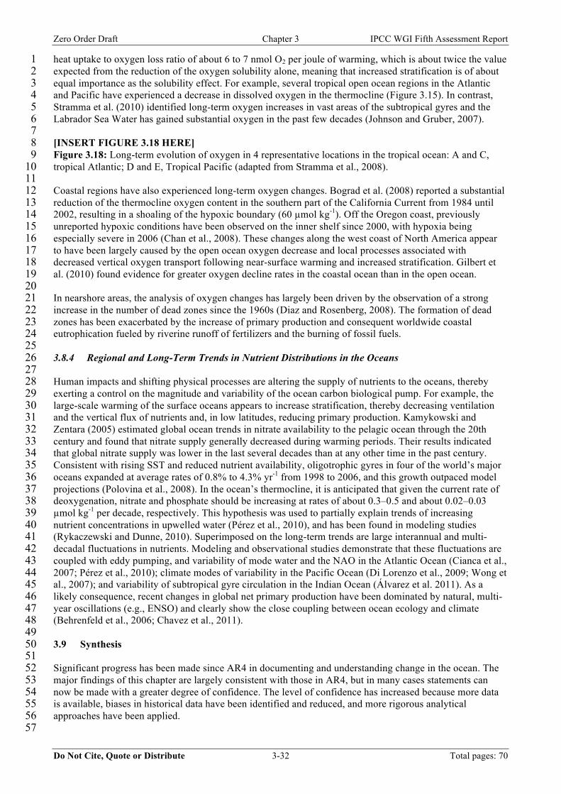
Zero Order Draft Chapter 3 IPCC WGI Fifth Assessment Report
Do Not Cite, Quote or Distribute 3-32 Total pages: 70
heat uptake to oxygen loss ratio of about 6 to 7 nmol O2 per joule of warming, which is about twice the value 1 expected from the reduction of the oxygen solubility alone, meaning that increased stratification is of about 2 equal importance as the solubility effect. For example, several tropical open ocean regions in the Atlantic 3 and Pacific have experienced a decrease in dissolved oxygen in the thermocline (Figure 3.15). In contrast, 4 Stramma et al. (2010) identified long-term oxygen increases in vast areas of the subtropical gyres and the 5 Labrador Sea Water has gained substantial oxygen in the past few decades (Johnson and Gruber, 2007). 6 7 [INSERT FIGURE 3.18 HERE] 8 Figure 3.18: Long-term evolution of oxygen in 4 representative locations in the tropical ocean: A and C, 9 tropical Atlantic; D and E, Tropical Pacific (adapted from Stramma et al., 2008). 10 11 Coastal regions have also experienced long-term oxygen changes. Bograd et al. (2008) reported a substantial 12 reduction of the thermocline oxygen content in the southern part of the California Current from 1984 until 13 2002, resulting in a shoaling of the hypoxic boundary (60 µmol kg-1). Off the Oregon coast, previously 14 unreported hypoxic conditions have been observed on the inner shelf since 2000, with hypoxia being 15 especially severe in 2006 (Chan et al., 2008). These changes along the west coast of North America appear 16 to have been largely caused by the open ocean oxygen decrease and local processes associated with 17 decreased vertical oxygen transport following near-surface warming and increased stratification. Gilbert et 18 al. (2010) found evidence for greater oxygen decline rates in the coastal ocean than in the open ocean. 19 20 In nearshore areas, the analysis of oxygen changes has largely been driven by the observation of a strong 21 increase in the number of dead zones since the 1960s (Diaz and Rosenberg, 2008). The formation of dead 22 zones has been exacerbated by the increase of primary production and consequent worldwide coastal 23 eutrophication fueled by riverine runoff of fertilizers and the burning of fossil fuels. 24 25 3.8.4 Regional and Long-Term Trends in Nutrient Distributions in the Oceans 26 27 Human impacts and shifting physical processes are altering the supply of nutrients to the oceans, thereby 28 exerting a control on the magnitude and variability of the ocean carbon biological pump. For example, the 29 large-scale warming of the surface oceans appears to increase stratification, thereby decreasing ventilation 30 and the vertical flux of nutrients and, in low latitudes, reducing primary production. Kamykowski and 31 Zentara (2005) estimated global ocean trends in nitrate availability to the pelagic ocean through the 20th 32 century and found that nitrate supply generally decreased during warming periods. Their results indicated 33 that global nitrate supply was lower in the last several decades than at any other time in the past century. 34 Consistent with rising SST and reduced nutrient availability, oligotrophic gyres in four of the world’s major 35 oceans expanded at average rates of 0.8% to 4.3% yr-1 from 1998 to 2006, and this growth outpaced model 36 projections (Polovina et al., 2008). In the ocean’s thermocline, it is anticipated that given the current rate of 37 deoxygenation, nitrate and phosphate should be increasing at rates of about 0.3–0.5 and about 0.02–0.03 38 µmol kg-1 per decade, respectively. This hypothesis was used to partially explain trends of increasing 39 nutrient concentrations in upwelled water (Pérez et al., 2010), and has been found in modeling studies 40 (Rykaczewski and Dunne, 2010). Superimposed on the long-term trends are large interannual and multi-41 decadal fluctuations in nutrients. Modeling and observational studies demonstrate that these fluctuations are 42 coupled with eddy pumping, and variability of mode water and the NAO in the Atlantic Ocean (Cianca et al., 43 2007; Pérez et al., 2010); climate modes of variability in the Pacific Ocean (Di Lorenzo et al., 2009; Wong et 44 al., 2007); and variability of subtropical gyre circulation in the Indian Ocean (Álvarez et al. 2011). As a 45 likely consequence, recent changes in global net primary production have been dominated by natural, multi-46 year oscillations (e.g., ENSO) and clearly show the close coupling between ocean ecology and climate 47 (Behrenfeld et al., 2006; Chavez et al., 2011). 48 49 3.9 Synthesis 50 51 Significant progress has been made since AR4 in documenting and understanding change in the ocean. The 52 major findings of this chapter are largely consistent with those in AR4, but in many cases statements can 53 now be made with a greater degree of confidence. The level of confidence has increased because more data 54 is available, biases in historical data have been identified and reduced, and more rigorous analytical 55 approaches have been applied. 56 57

Zero Order Draft Chapter 3 IPCC WGI Fifth Assessment Report
Do Not Cite, Quote or Distribute 3-33 Total pages: 70
It is virtually certain that the oceans have warmed since 1970. More than 93% of the extra energy stored by 1 the Earth system over the last 50 years is found in the oceans. Correction of biases in older XBT data reveals 2 a greater and more continuous rate of warming, in better agreement with climate model simulations of the 3 20th century. Warming has been largest near the sea surface, increasing the thermal stratification of the 4 upper ocean. The warming of the ocean between 1961 and 2003 caused a thermosteric rise in sea level of 5 0.5±0.1 mm yr-1, an increase of 40% over earlier assessments that were affected by instrumental biases. 6 Significant, spatially coherent changes in surface salinity have been observed over much of the global ocean. 7 The spatial pattern of change in surface salinity has acted to reinforce the mean salinity pattern, and is 8 similar to the distribution of evaporation – precipitation, consistent with an increase in intensity of the 9 hydrological cycle. Changes in salinity penetrate to depths of 2000 m in many parts of the world ocean, 10 reflecting subduction of surface salinity anomalies produced by changes in freshwater flux and by migration 11 of density surfaces caused by warming. 12 13 Observations of changes in ocean circulation have increased in number and quality since AR4, but the time 14 series are still too short to reveal significant trends given the presence of energetic variability revealed by the 15 records. Much of the variability observed in the ocean circulation can be linked to changes in wind forcing, 16 including wind changes associated with the major modes of climate variability such as NAO, SAM, ENSO, 17 and the PDO. 18 19 Three independent methods confirm that the oceans continue to absorb about 25% of anthropogenic 20 emissions of CO2. The ocean inventory of anthropogenic CO2 increased from 114 ± 22 PgC to 140 ± 25 PgC 21 between 1994 and 2008. The uptake of anthropogenic CO2 is virtually certain to have caused acidification of 22 the ocean, with pH in the surface mixed layer having decreased by between -0.0018 and -0.0005 per year. 23 Other chemical changes observed in the ocean include widespread deoxygenation of the ocean thermocline 24 at a rate of 3–5 µmol kg-1 per decade and a possible increase in nutrient concentrations. 25 26 Observed changes in the ocean are summarised in a schematic in Figure X (in preparation). Taken together, 27 the observations summarised here give very high confidence that the physical and chemical state of the 28 oceans has changed. The spatial patterns of change are consistent with changes in the surface ocean 29 (warming, changes in freshwater flux and an increase in Cant) and the subsequent propagation of anomalies 30 into the ocean interior along ventilation pathways. The consistency of the observed patterns of change with 31 known physical and chemical processes in the ocean enhances the level of confidence associated with the 32 conclusion that the ocean state has changed. 33 34 Improvements in the quality and quantity of ocean observations strengthen conclusions reached in AR4, but 35 substantial uncertainties remain. In many cases, the observational record is too short or incomplete to detect 36 trends in the presence of energetic variability on time-scales of years to decades. Recent improvements in the 37 ocean observing system, most notably the Argo profiling float array, mean that temperature and salinity are 38 now being sampled routinely in most of the global ocean above 2000 m depth for the first time. If these 39 observations are sustained, and complemented with time series, measurements of the deep ocean and 40 expanded biogeochemical sampling, the evolution of ocean climate will be able to be assessed with greater 41 confidence. 42 43 44 [START FAQ 3.1 HERE] 45 46 FAQ 3.1: Is the Ocean Warming? 47 48 Yes, the ocean is warming, and an important part of climate change. Over time scales longer than a decade 49 the average temperature of the upper ocean has increased at least since 1970, when data coverage began to 50 be adequate for estimating global averages. Observations suggest that the coldest waters at the bottom of the 51 ocean have been warming overall since around 1990. 52 53 Ocean temperature in a given location can vary largely with the march of the seasons and can also fluctuate 54 substantially from year-to-year or even decade-to-decade owing to variability in the heat exchange between 55 ocean and atmosphere as well as variations in ocean currents. But when we average over longer times and 56 larger regions, an upward trend in ocean heat content becomes increasingly apparent. 57

Zero Order Draft Chapter 3 IPCC WGI Fifth Assessment Report
Do Not Cite, Quote or Distribute 3-34 Total pages: 70
1 Archived historical ocean temperature measurements extend back for centuries, but not until around 1970 are 2 the measurements in any given year sufficient in number and sufficiently global in their spatial distribution 3 to estimate global upper ocean temperature with confidence. Until the Argo program first achieved global 4 coverage in 2004, the global average upper ocean temperature anomaly for any given year is sensitive to the 5 methodology used to estimate it. In spite of the large uncertainty, the increase of the global mean over 6 decadal time scales since 1970 is a robust result. 7 8 Temperature anomalies enter the subsurface ocean by multiple paths (FAQ3.1, Figure 1). In addition to 9 mixing from above, colder waters from high latitude regions can sink down from the surface and slide 10 equatorward under warmer waters from more tropical regions. As these sinking waters become warmer, they 11 increase temperatures in the deep ocean much more quickly than would downward mixing of surface heating 12 alone. There are a few locations — in the Northern North Atlantic and around Antarctica — where ocean 13 water is cooled enough so that it sinks to great depths, even to the ocean bottom. It spreads out from these 14 locations to fill much of the rest of the deep ocean. The temperature of these deep waters varies from decade 15 to decade in the North Atlantic, sometimes warming, sometimes cooling, depending on the prevailing winter 16 atmospheric patterns there. Around Antarctica, the bottom waters appear to have been warming relatively 17 fast since at least 1990, perhaps owing to the strengthening and poleward shift of the westerly winds around 18 the Southern Ocean over the last several decades. 19 20 [INSERT FAQ 3.1, FIGURE 1 HERE] 21 FAQ 3.1, Figure 1: Ocean warming pathways. The ocean is stratified, with the coldest water, Antarctic 22 Bottom Water (dark blue) sinking around Antarctica and spreading northward along the ocean floor into the 23 central Pacific (bottom panel, left) and western Atlantic (bottom panel, right) oceans, as well as the Indian 24 Ocean (not shown). North Atlantic Deep Water (lighter blue) sinks in the northern North Atlantic Ocean and 25 spreads south above the Antarctic Bottom Water and then around Antarctica and into the Pacific and Indian 26 Oceans. Similarly, in the upper ocean (top left panel) Intermediate Waters (cyan) sink in subpolar regions 27 and slip equatorward under Subtropical Waters (green), which in turn slip equatorward under tropical waters 28 (orange) in all three oceans. Excess heat entering at the ocean surface also mixes slowly downward (squiggly 29 red arrows). 30 31 From the ocean surface to about 60-m depth, the global average rate of ocean warming has been around 32 0.1°C per decade from 1967–2009. The global average rate of ocean warming generally gets smaller with 33 increasing depth, reducing to about 0.04°C per decade by 200 m and under 0.02°C per decade by 500 m. 34 While the deep warming rates can be small (for instance about 0.03°C per decade since the 1990s in the deep 35 and bottom waters around Antarctica), they occur over a large volume, so the deep ocean warming 36 contributes a notable fraction to the total increase in ocean heat content. To put the huge heat capacity of the 37 ocean into context, and the ocean’s overall role in climate, the estimated energy it has absorbed between 38 1970 and 2003 is about 93% of the total heat gain by the combined air, sea, land, and cryosphere that make 39 up the climate system. In other words, as the Earth is absorbing more heat than it is emitting back into space, 40 nearly all of the excess heat is entering the oceans. 41 42 Estimates of change in global average ocean temperature have improved since AR4 was published in 2007, 43 largely through reductions in systematic measurement errors. Careful comparison of less accurate 44 measurements with sparser but more accurate ones at nearby locations and times has made the historical 45 record more consistent and removed spurious variability. With the biases ameliorated, it is seen that the 46 global average ocean temperature has increased much more steadily from year to year than what was 47 reported in AR4. However, the global average warming rate may not be uniform in time: There are years 48 when it appears faster than average, and years where it seems to slow to almost nothing. 49 50 The ocean’s large mass and high heat capacity (their product is over 1000 times the atmosphere’s) mean that 51 it can store huge amounts of energy. This fact, coupled with its long time-scales for exchange of water from 52 the surface to its depths, means that the ocean has significant thermal inertia. It takes decades for near-53 surface ocean temperatures to adjust in response to climate forcing such as changes in greenhouse gas 54 concentrations. It will take centuries to millennia for deep ocean temperatures to warm in response to 55 changes occurring today. Thus, even if greenhouse gas concentrations could be held constant at their present 56 levels into the future, Earth’s surface would continue to warm for decades. Furthermore, sea level would 57

Zero Order Draft Chapter 3 IPCC WGI Fifth Assessment Report
Do Not Cite, Quote or Distribute 3-35 Total pages: 70
continue to rise for centuries to millennia as the deep oceans continued to warm and expand (even absent the 1 contributions of melting land ice). 2 3 [END FAQ 3.1 HERE] 4 5 6 [START FAQ 3.2 HERE] 7 8 FAQ 3.2: How Does Anthropogenic Ocean Acidification Relate to Climate Change? 9 10 Anthropogenic ocean acidification refers to an increase in the ocean’s hydrogen ion concentration (in other 11 words, a lowering of pH or increase in acidity) caused by human activities, including the uptake of 12 atmospheric carbon dioxide (CO2) derived from the burning of fossil fuels, land-use changes, and cement 13 production. Implicit with the pH change are the associated changes in the concentrations of the dissolved 14 carbon species (CO2(aq), H2CO3, HCO3
-, CO32-). Results from laboratory, field, and modeling studies, as well 15
as evidence from the geological record, clearly indicate that marine ecosystems are highly susceptible to the 16 increases in oceanic CO2 and the corresponding decreases in pH (Doney et al., 2009). Ocean acidification 17 describes the direction of pH change rather than the end point; that is, ocean pH is decreasing but is not 18 expected to become acidic (pH<7). 19 20 Both climate change and anthropogenic ocean acidification are caused by increasing carbon dioxide 21 concentration in the atmosphere. Rising levels of CO2, along with other greenhouse gases, indirectly alter the 22 climate system by trapping heat that perturbs the Earth’s radiation budget. Anthropogenic ocean acidification 23 is a direct consequence of rising CO2 concentrations as seawater absorbs CO2 from the atmosphere. Climate 24 change and anthropogenic ocean acidification do not act independently, as both processes affect the 25 exchange of CO2 between the atmosphere and ocean. CO2 stored in the ocean does not contribute to 26 greenhouse warming. However, the solubility of carbon dioxide in seawater decreases with increasing 27 temperature; ocean warming thus reduces the amount of CO2 the oceans can absorb from the atmosphere. 28 For example, under doubled preindustrial CO2 concentrations and a 2°C temperature increase, seawater 29 absorbs about 10% less CO2 than it would with no temperature increase (FAQ 3.2, Table 1). Temperature 30 has a much smaller effect on pH; under doubled CO2 conditions, a 2°C increase reduces the pH shift by less 31 than 1% (FAQ 3.2, Table 1). Thus, a warmer ocean is less efficient at reducing greenhouse warming in the 32 atmosphere, but still experiences ocean acidification. 33 34 35 FAQ 3.2, Table 1: Oceanic pH and carbon system parameter changes for a CO2 doubling from the preindustrial 36 atmosphere without and with a 2°C warming. 37 Parameter preindustrial
(280 ppmv) 20°C
2x preindustrial (560 ppmv) 20°C
% change relative to preindustrial
2x preindustrial (560 ppmv) 22°C
% change relative to preindustrial
pH 8.17 7.92 -3.1 7.92 -3.1 CO2* (µmol kg -1) 9.04 18.09 100.0 17.13 89.4 HCO3
- (µmol kg -1) 1727.51 1939.50 12.3 1916.78 11.0 CO3
2- (µmol kg -1) 231.68 146.02 -37.0 155.50 -32.9 DIC (µmol kg -1) 1968.23 2103.60 6.9 2089.41 6.2 38 [END FAQ 3.2 HERE] 39 40 41 [START FAQ 3.3 HERE] 42 43 FAQ 3.3: Is There Evidence for Changes in the Earth’s Water Cycle? 44 45 The Earth’s water cycle involves evaporation and precipitation of moisture at the Earth’s surface. Most of 46 the exchange of freshwater between the atmosphere and the surface takes place over the 70% of the Earth’s 47 surface that is covered by ocean. The water cycle is expected to intensify in a warmer climate, because warm 48

Zero Order Draft Chapter 3 IPCC WGI Fifth Assessment Report
Do Not Cite, Quote or Distribute 3-36 Total pages: 70
air can hold more moisture: the atmosphere can hold about 7% more water vapor for each degree C of 1 warming. 2 3 Directly observing a change in the water cycle is difficult, however, because observations of precipitation 4 and evaporation are sparse and uncertain, particularly over the ocean where most of the exchange of 5 moisture occurs. The uncertainties are so large in the individual terms that it is not possible to detect robust 6 trends from these observations. Ocean salinity, on the other hand, naturally integrates the net freshwater flux 7 resulting from the difference between precipitation and evaporation and can therefore act as a sensitive and 8 effective rain gauge. (Ocean salinity can also be affected by run-off of water from the continents and by the 9 melting and freezing of sea ice or floating glacial ice.) 10 11 The distribution of salinity at the ocean surface largely mirrors the distribution of evaporation – precipitation. 12 High salinity is observed in the subtropics, where evaporation exceeds precipitation, and low salinity is 13 observed at high latitudes and in the tropics, where there is more rainfall than evaporation. The Atlantic, the 14 saltiest ocean basin, loses more freshwater through evaporation than it gains from precipitation, while the 15 reverse is true for the Pacific. Transport of moisture as water vapor in the atmosphere connects the regions of 16 net freshwater gain or loss by the ocean. 17 18 Changes observed in ocean salinity in the last 50 years provide strong evidence that the global water cycle is 19 increasing in intensity as the Earth warms, as anticipated from the fact that warmer air can hold more 20 moisture. Changes in surface salinity have reinforced the mean salinity pattern: the evaporation-dominated 21 subtropical regions have become saltier, while the precipitation-dominated subpolar and tropical regions 22 have become fresher. The observed changes in surface salinity are statistically significant at the 99% level of 23 confidence over more than 40% of the surface of the global ocean (Durack and Wijffels, 2010). 24 25 [The rest of this FAQ requires input from other chapters on evidence for changes in the water cycle based on 26 land observations.] 27 28 [END FAQ 3.3 HERE] 29 30
31

Zero Order Draft Chapter 3 IPCC WGI Fifth Assessment Report
Do Not Cite, Quote or Distribute 3-37 Total pages: 70
References 1 Abeysirigunawardena, D. S., and I. J. Walker, 2008: Sea Level Responses to Climatic Variability and Change in 2
Northern British Columbia. Atmosphere-Ocean, 46, 277-296. 3 Álvarez et al., M., 2011: Decadal biogeochemical changes in the western Indian Ocean associated with Subantarctic 4
Mode Water. Journal of Geophysical Research, resubmitted. 5 Andersson, A., C. Klepp, K. Fennig, S. Bakan, H. Graßl, and J. Schulz, 2010: Evaluation of HOAPS-3 ocean surface 6
freshwater flux components. Journal of Applied Meteorology and Climatology, in press. 7 Andersson et al, A., 2011, in preparation. 8 Andrié, C., Y. Gouriou, B. Bourlès, J. F. Ternon, E. S. Braga, P. Morin, and C. Oudot, 2003: Variability of AABW 9
properties in the equatorial channel at 35°W. Geophys. Res. Lett., 30, 8007. 10 Antonov, J. I., S. Levitus, and T. P. Boyer, 2002: Steric sea level variations during 1957-1994: Importance of salinity. 11
Journal of Geophysical Research-Oceans, 107. 12 ——, 2005: Thermosteric sea level rise, 1955-2003. Geophysical Research Letters, 32. 13 Aoki, S., S. R. Rintoul, S. Ushio, S. Watanabe, and N. L. Bindoff, 2005: Freshening of the Adelie Land Bottom Water 14
near 140 degrees E. Geophysical Research Letters, 32. 15 Bates, N. R., 2007: Interannual variability of the oceanic CO2 sink in the subtropical gyre of the North Atlantic Ocean 16
over the last 2 decades. Journal of Geophysical Research-Oceans, 112, -. 17 Beckley, B. D., et al., 2010: Assessment of the Jason-2 Extension to the TOPEX/Poseidon, Jason-1 Sea-Surface Height 18
Time Series for Global Mean Sea Level Monitoring. Marine Geodesy, 33, 447-471. 19 Behrenfeld, M. J., et al., 2006: Climate-driven trends in contemporary ocean productivity. Nature, 444, 752-755. 20 Bersch, M., I. Yashayaev, and K. P. Koltermann, 2007: Recent changes of the thermohaline circulation in the subpolar 21
North Atlantic. Ocean Dynamics, 57, 223-235. 22 Berx, B., S. L. Hughes, B. Hansen, S. Sterhus, and T. Sherwin, 2011: Fluxes of Atlantic Water (Volume, Heat and Salt) 23
in the Faroe-Shetland Channel calculated from over a decade of Acoustic Current Profiler Data (1994-2008). in 24 prep. 25
Bindoff, N. L., and T. J. McDougall, 1994: DIAGNOSING CLIMATE-CHANGE AND OCEAN VENTILATION 26 USING HYDROGRAPHIC DATA. Journal of Physical Oceanography, 24, 1137-1152. 27
Bindoff, N. L., et al., 2007: Observations: Oceanic Climate Change and Sea Level. Climate Change 2007: The Physical 28 Science Basis. Contribution of Working Group I to the Fourth Assessment Report of the Intergovernmental 29 Panel on Climate Change, S. Solomon, et al., Eds., Cambridge University Press. 30
Bograd, S. J., C. G. Castro, E. Di Lorenzo, D. M. Palacios, H. Bailey, W. Gilly, and F. P. Chavez, 2008: Oxygen 31 declines and the shoaling of the hypoxic boundary in the California Current. Geophysical Research Letters, 35. 32
Boning, C. W., A. Dispert, M. Visbeck, S. R. Rintoul, and F. U. Schwarzkopf, 2008: The response of the Antarctic 33 Circumpolar Current to recent climate change. Nature Geoscience, 1, 864-869. 34
Boyer, T., S. Levitus, J. Antonov, R. Locarnini, A. Mishonov, H. Garcia, and S. A. Josey, 2007: Changes in freshwater 35 content in the North Atlantic Ocean 1955-2006. Geophysical Research Letters, 34. 36
Boyer, T. P., S. Levitus, J. I. Antonov, R. A. Locarnini, and H. E. Garcia, 2005: Linear trends in salinity for the World 37 Ocean, 1955-1998. Geophysical Research Letters, 32. 38
Boyer, T. P., et al., 2009: World Ocean Database 2009, 216 pp. 39 Bryden, H. L., H. R. Longworth, and S. A. Cunningham, 2005: Slowing of the Atlantic meridional overturning 40
circulation at 25 degrees N. Nature, 438, 655-657. 41 Byrne, R. H., S. Mecking, R. A. Feely, and X. W. Liu, 2010: Direct observations of basin-wide acidification of the 42
North Pacific Ocean. Geophysical Research Letters, 37. 43 Cai, W., 2006: Antarctic ozone depletion causes an intensification of the Southern Ocean super-gyre circulation. 44
Geophysical Research Letters, 33. 45 Caldeira, K., and M. E. Wickett, 2003: Anthropogenic carbon and ocean pH. Nature, 425, 365-365. 46 Carson, M., and D. E. Harrison, 2010: Regional Interdecadal Variability in Bias-Corrected Ocean Temperature Data. 47
Journal of Climate, 23, 2847-2855. 48 Carton, J. A., and A. Santorelli, 2008: Global Decadal Upper-Ocean Heat Content as Viewed in Nine Analyses. Journal 49
of Climate, 21, 6015-6035. 50 Carton, J. A., B. S. Giese, and S. A. Grodsky, 2005: Sea level rise and the warming of the oceans in the Simple Ocean 51
Data Assimilation (SODA) ocean reanalysis. Journal of Geophysical Research-Oceans, 110. 52 Cazenave, A., and R. S. Nerem, 2004: Present-day sea level change: Observations and causes. Reviews of Geophysics, 53
42. 54 Cazenave, A., A. Lombard, and W. Llovel, 2008: Present-day sea level rise: A synthesis. Comptes Rendus Geoscience, 55
340, 761-770. 56 Cazenave, A., et al., 2009: Sea level budget over 2003–2008: A re-evaluation from GRACE space gravimetry, satellite 57
altimetry and Argo. Marine Geodesy, 65, 447 - 471. 58 Cermak, J., M. Wild, R. Knutti, M. I. Mishchenko, and A. K. Heidinger, 2010: Consistency of global satellite-derived 59
aerosol and cloud data sets with recent brightening observations. Geophysical Research Letters, 37. 60 Chambers, D. P., J. Wahr, and R. S. Nerem, 2004: Preliminary observations of global ocean mass variations with 61
GRACE. Geophysical Research Letters, 31. 62

Zero Order Draft Chapter 3 IPCC WGI Fifth Assessment Report
Do Not Cite, Quote or Distribute 3-38 Total pages: 70
Chambers, D. P., J. Wahr, M. E. Tamisiea, and R. S. Nerem, 2010: Ocean mass from GRACE and glacial isostatic 1 adjustment. Journal of Geophysical Research-Solid Earth, 115. 2
Chan, F., J. A. Barth, J. Lubchenco, A. Kirincich, H. Weeks, W. T. Peterson, and B. A. Menge, 2008: Emergence of 3 anoxia in the California current large marine ecosystem. Science, 319, 920-920. 4
Chavez, F. P., M. Messié, and J. T. Pennington, 2011: Marine primary production in relation to climate variability and 5 change. Annual Review of Marine Science, 3, 227-260. 6
Church, J. A., and N. J. White, 2006: A 20th century acceleration in global sea-level rise. Geophysical Research Letters, 7 33. 8
Church, J. A., N. J. White, and J. M. Arblaster, 2005: Significant decadal-scale impact of volcanic eruptions on sea 9 level and ocean heat content. Nature, 438, 74-77. 10
Church, J. A., J. R. Hunter, K. L. McInnes, and N. J. White, 2006: Sea-level rise around the Australian coastline and the 11 changing frequency of extreme sea-level events. Australian Meteorological Magazine, 55, 253-260. 12
Church, J. A., N. J. White, R. Coleman, K. Lambeck, and J. X. Mitrovica, 2004: Estimates of the regional distribution 13 of sea level rise over the 1950-2000 period. Journal of Climate, 17, 2609-2625. 14
Cianca, A., P. Helmke, B. Mourino, M. J. Rueda, O. Llinas, and S. Neuer, 2007: Decadal analysis of hydrography and 15 in situ nutrient budgets in the western and eastern North Atlantic subtropical gyre. Journal of Geophysical 16 Research-Oceans, 112. 17
Cooley, S. R., H. L. Kite-Powell, and S. C. Doney, 2009: Ocean Acidification's Potential to Alter Global Marine 18 Ecosystem Services. Oceanography, 22, 172-181. 19
Cravatte, S., T. Delcroix, D. X. Zhang, M. McPhaden, and J. Leloup, 2009: Observed freshening and warming of the 20 western Pacific Warm Pool. Climate Dynamics, 33, 565-589. 21
Cummins, P. F., and H. J. Freeland, 2007: Variability of the North Pacific current and its bifurcation. Progress in 22 Oceanography, 75, 253-265. 23
Cunningham, S., et al., 2010: The present and future system for measuring the Atlantic meridional overturning 24 circulation and heat transport. Proceedings of OceanObs’09: Sustained Ocean Observations and Information for 25 Society (Vol. 2), Venice, Italy, European Space Agency Publication, 16. 26
Cunningham, S. A., S. G. Alderson, B. A. King, and M. A. Brandon, 2003: Transport and variability of the Antarctic 27 Circumpolar Current in Drake Passage. Journal of Geophysical Research-Oceans, 108. 28
Cunningham, S. A., et al., 2007: Temporal variability of the Atlantic meridional overturning circulation at 26.5 degrees 29 N. Science, 317, 935-938. 30
Curry, R., and C. Mauritzen, 2005: Dilution of the northern North Atlantic Ocean in recent decades. Science, 308, 31 1772-1774. 32
Curry, R., B. Dickson, and I. Yashayaev, 2003: A change in the freshwater balance of the Atlantic Ocean over the past 33 four decades. Nature, 426, 826-829. 34
D'Onofrio, E. E., M. M. E. Fiore, and J. L. Pousa, 2008: Changes in the regime of storm surges at Buenos Aires, 35 Argentina. Journal of Coastal Research, 24, 260-265. 36
Delcroix, T., S. Cravatte, and M. J. McPhaden, 2007: Decadal variations and trends in tropical Pacific sea surface 37 salinity since 1970. Journal of Geophysical Research-Oceans, 112. 38
Deng, Z. W., and Y. M. Tang, 2009: Reconstructing the Past Wind Stresses over the Tropical Pacific Ocean from 1875 39 to 1947. Journal of Applied Meteorology and Climatology, 48, 1181-1198. 40
Di Lorenzo, E., et al., 2009: Nutrient and salinity decadal variations in the central and eastern North Pacific. 41 Geophysical Research Letters, 36. 42
Diaz, R. J., and R. Rosenberg, 2008: Spreading dead zones and consequences for marine ecosystems. Science, 321, 43 926-929. 44
Dickson, B., I. Yashayaev, J. Meincke, B. Turrell, S. Dye, and J. Holfort, 2002: Rapid freshening of the deep North 45 Atlantic Ocean over the past four decades. Nature, 416, 832-837. 46
Dmitrenko, I. A., et al., 2008: Toward a warmer Arctic Ocean: Spreading of the early 21st century Atlantic Water warm 47 anomaly along the Eurasian Basin margins. Journal of Geophysical Research-Oceans, 113, 13. 48
Dodet, G., X. Bertin, and R. Taborda, 2010: Wave climate variability in the North-East Atlantic Ocean over the last six 49 decades. Ocean Modelling, 31, 120-131. 50
Dohan, K., et al., 2010: Measuring the Global Ocean Surface Circulation with Satellite and In Situ Observations. 51 Proceedings of OceanObs’09: Sustained Ocean Observations and Information for Society (Vol. 2), Venice, Italy. 52
Domingues, C. M., J. A. Church, N. J. White, P. J. Gleckler, S. E. Wijffels, P. M. Barker, and J. R. Dunn, 2008: 53 Improved estimates of upper-ocean warming and multi-decadal sea-level rise. Nature, 453, 1090-U1096. 54
Doney, S. C., V. J. Fabry, R. A. Feely, and J. A. Kleypas, 2009: Ocean Acidification: The Other CO2 Problem. Annual 55 Review of Marine Science, 1, 169-192. 56
Dore, J. E., R. Lukas, D. W. Sadler, M. J. Church, and D. M. Karl, 2009: Physical and biogeochemical modulation of 57 ocean acidification in the central North Pacific. Proceedings of the National Academy of Sciences of the United 58 States of America, 106, 12235-12240. 59
Douglass, E., D. Roemmich, and D. Stammer, 2006: Interannual variability in northeast pacific circulation. Journal of 60 Geophysical Research-Oceans, 111. 61
Ducet, N., P. Y. Le Traon, and G. Reverdin, 2000: Global high-resolution mapping of ocean circulation from 62 TOPEX/Poseidon and ERS-1 and-2. Journal of Geophysical Research-Oceans, 105, 19477-19498. 63

Zero Order Draft Chapter 3 IPCC WGI Fifth Assessment Report
Do Not Cite, Quote or Distribute 3-39 Total pages: 70
Durack, P. J., and S. E. Wijffels, 2010: Fifty-Year Trends in Global Ocean Salinities and Their Relationship to Broad-1 Scale Warming. Journal of Climate, 23, 4342-4362. 2
Egleston, E. S., C. L. Sabine, and F. M. M. Morel, 2010: Revelle revisited: Buffer factors that quantify the response of 3 ocean chemistry to changes in DIC and alkalinity. Global Biogeochemical Cycles, 24. 4
Fabry, V. J., B. A. Seibel, R. A. Feely, and J. C. Orr, 2008: Impacts of ocean acidification on marine fauna and 5 ecosystem processes. Ices Journal of Marine Science, 65, 414-432. 6
Feely, R. A., S. C. Doney, and S. R. Cooley, 2009: Ocean Acidification: Present Conditions and Future Changes in a 7 High-CO2 World. Oceanography, 22, 36-47. 8
Feely, R. A., C. L. Sabine, K. Lee, W. Berelson, J. Kleypas, V. J. Fabry, and F. J. Millero, 2004: Impact of 9 anthropogenic CO2 on the CaCO3 system in the oceans. Science, 305, 362-366. 10
Feely, R. A., T. Takahashi, R. Wanninkhof, M. J. McPhaden, C. E. Cosca, S. C. Sutherland, and M. E. Carr, 2006: 11 Decadal variability of the air-sea CO2 fluxes in the equatorial Pacific Ocean. Journal of Geophysical Research-12 Oceans, 111, -. 13
Fischer, J., M. Visbeck, R. Zantopp, and N. Nunes, 2010: Interannual to decadal variability of outflow from the 14 Labrador Sea. Geophysical Research Letters, 37. 15
Freeland, H., et al., 2010: Argo - A Decade of Progress. Proceedings of OceanObs’09: Sustained Ocean Observations 16 and Information for Society (Vol. 2), Venice, Italy. 17
Friis, K., A. Körtzinger, J. Pätsch, and D. W. R. Wallace, 2005: On the temporal increase of anthropogenic CO2 in the 18 subpolar North Atlantic. Deep-Sea Research I, 52, 681-698. 19
Fukasawa, M., H. Freeland, R. Perkin, T. Watanabe, J. Uchida, and A. Nishina, 2004: Bottom water warming in the 20 North Pacific Ocean. 825–827. 21
Fusco, G., V. Artale, Y. Cotroneo, and G. Sannino, 2008: Thermohaline variability of Mediterranean Water in the Gulf 22 of Cadiz, 1948-1999. Deep-Sea Research Part I-Oceanographic Research Papers, 55, 1624-1638. 23
Ganachaud, A., and C. Wunsch, 2003: Large-scale ocean heat and freshwater transports during the World Ocean 24 Circulation Experiment. Journal of Climate, 16, 696-705. 25
Garabato, A. C. N., L. Jullion, D. P. Stevens, K. J. Heywood, and B. A. King, 2009: Variability of Subantarctic Mode 26 Water and Antarctic Intermediate Water in the Drake Passage during the Late-Twentieth and Early-Twenty-First 27 Centuries. Journal of Climate, 22, 3661-3688. 28
Giese, B. S., G. A. Chepurin, J. A. Carton, T. P. Boyer, and H. F. Seidel, 2011: Impact of bathythermograph 29 temperature bias models on an ocean reanalysis. Journal of Climate, 24, 84-93. 30
Gilbert, D., N. N. Rabalais, R. J. Diaz, and J. Zhang, 2010: Evidence for greater oxygen decline rates in the coastal 31 ocean than in the open ocean. Biogeosciences, 7, 2283-2296. 32
Gille, S. T., 2008: Decadal-scale temperature trends in the Southern Hemisphere ocean. Journal of Climate, 21, 4749-33 4765. 34
Gladyshev, S. V., M. N. Koshlyakov, and R. Y. Tarakanov, 2008: Currents in the Drake Passage based on observations 35 in 2007. Oceanology, 48, 759-770. 36
Gonzalez-Davila, M., J. M. Santana-Casiano, M. J. Rueda, and O. Llinas, 2010: The water column distribution of 37 carbonate system variables at the ESTOC site from 1995 to 2004. Biogeosciences, 7, 3067-3081. 38
Gouretski, V., and K. P. Koltermann, 2007: How much is the ocean really warming? Geophysical Research Letters, 34, 39 5. 40
Gouretski, V., and F. Reseghetti, 2010: On depth and temperature biases in bathythermograph data: Development of a 41 new correction scheme based on analysis of a global ocean database. Deep-Sea Research Part I-Oceanographic 42 Research Papers, 57, 812-833. 43
Grigorieva, V., and S. K. Gulev, 2011: Changes in wind wave periods and steepness over global ocean from the VOS 44 data. Journal of Climate, submitted. 45
Grist, J., R. Marsh, and S. Josey, 2009: On the Relationship between the North Atlantic Meridional Overturning 46 Circulation and the Surface-Forced Overturning Streamfunction. Journal of Climate, 4989-5002. 47
Gu, G. J., R. F. Adler, G. J. Huffman, and S. Curtis, 2007: Tropical rainfall variability on interannual-to-interdecadal 48 and longer time scales derived from the GPCP monthly product. Journal of Climate, 20, 4033-4046. 49
Gulev, S., T. Jung, and E. Ruprecht, 2007: Estimation of the impact of sampling errors in the VOS observations on air-50 sea fluxes. Part II: Impact on trends and interannual variability. Journal of Climate, 20, 302-315. 51
Gulev, S., et al., 2010: Surface Energy and CO2 Fluxes in the Global Ocean-Atmosphere-Ice System. OceanObs'09: 52 Sustained Ocean Observations and Information for Society, Venice, Italy, 20 pp. 53
Gulev, S. K., and V. Grigorieva, 2006: Variability of the winter wind waves and swell in the North Atlantic and North 54 Pacific as revealed by the voluntary observing ship data. Journal of Climate, 19, 5667-5685. 55
——, 2011: Long-term variability in extreme wind waves estimated from the VOS data. Journal of Geophysical 56 Research, submitted. 57
Gulev, S. K., and K. P. Belyaev, 2011: Probability distribution characteristics for surface air-sea turbulent heat fluxes 58 over the global ocean. Journal of Climate, in revision. 59
Haigh, I., R. Nicholls, and N. Wells, 2010: Assessing changes in extreme sea levels: Application to the English 60 Channel, 1900-2006. Continental Shelf Research, 30, 1042-1055. 61
Hakkinen, S., and P. B. Rhines, 2009: Shifting surface currents in the northern North Atlantic Ocean. Journal of 62 Geophysical Research-Oceans, 114. 63

Zero Order Draft Chapter 3 IPCC WGI Fifth Assessment Report
Do Not Cite, Quote or Distribute 3-40 Total pages: 70
Hakkinen, S., A. Proshutinsky, and I. Ashik, 2008: Sea ice drift in the Arctic since the 1950s. Geophysical Research 1 Letters, 35. 2
Hansen, J., et al., 2005: Earth's energy imbalance: Confirmation and implications. Science, 308, 1431-1435. 3 Hatun, H., A. B. Sando, H. Drange, B. Hansen, and H. Valdimarsson, 2005: Influence of the Atlantic subpolar gyre on 4
the thermohaline circulation. Science, 309, 1841-1844. 5 Held, I. M., and B. J. Soden, 2006: Robust responses of the hydrological cycle to global warming. Journal of Climate, 6
19, 5686-5699. 7 Helm, K. P., N. L. Bindoff, and J. A. Church, 2010: Changes in the global hydrological-cycle inferred from ocean 8
salinity. Geophysical Research Letters, 37. 9 Hemer, M. A., 2010: Historical trends in Southern Ocean storminess: Long-term variability of extreme wave heights at 10
Cape Sorell, Tasmania. Geophysical Research Letters, 37. 11 Hemer, M. A., J. A. Church, and J. R. Hunter, 2010: Variability and trends in the directional wave climate of the 12
Southern Hemisphere. International Journal of Climatology, 30, 475-491. 13 Hill, K. L., S. R. Rintoul, R. Coleman, and K. R. Ridgway, 2008: Wind forced low frequency variability of the East 14
Australia Current. Geophysical Research Letters, 35. 15 Hinkelman, L. M., P. W. Stackhouse, B. A. Wielicki, T. P. Zhang, and S. R. Wilson, 2009: Surface insolation trends 16
from satellite and ground measurements: Comparisons and challenges. Journal of Geophysical Research-17 Atmospheres, 114. 18
Holgate, S. J., 2007: On the decadal rates of sea level change during the twentieth century. Geophysical Research 19 Letters, 34. 20
Holland, P. R., A. Jenkins, and D. M. Holland, 2008: The response of ice shelf basal melting to variations in ocean 21 temperature. Journal of Climate, 21, 2558-2572. 22
Holliday, N., et al., 2008: Reversal of the 1960s to 1990s freshening trend in the northeast North Atlantic and Nordic 23 Seas. Geophysical Research Letters, -. 24
Hood, M., et al., 2010: Ship-based Repeat Hydrography: A Strategy for a Sustained Global Program. Proceedings of 25 OceanObs’09: Sustained Ocean Observations and Information for Society (Vol. 2), Venice, Italy. 26
Hosoda, S., T. Suga, N. Shikama, and K. Mizuno, 2009: Global Surface Layer Salinity Change Detected by Argo and 27 Its Implication for Hydrological Cycle Intensification. Journal of Oceanography, 65, 579-586. 28
Ishii, M., and M. Kimoto, 2009: Reevaluation of historical ocean heat content variations with time-varying XBT and 29 MBT depth bias corrections. Journal of Oceanography, 65, 287-299. 30
Jackson, J. M., E. C. Carmack, F. A. McLaughlin, S. E. Allen, and R. G. Ingram, 2010: Identification, characterization, 31 and change of the near-surface temperature maximum in the Canada Basin, 1993-2008. Journal of Geophysical 32 Research-Oceans, 115, 16. 33
Jacobs, S., 2004: Bottom water production and its links with the thermohaline circulation. Antarctic Science, 427-437. 34 ——, 2006: Observations of change in the Southern Ocean. Philosophical Transactions of the Royal Society a-35
Mathematical Physical and Engineering Sciences, 364, 1657-1681. 36 Jacobs, S. S., and C. F. Giulivi, 2010: Large Multidecadal Salinity Trends near the Pacific-Antarctic Continental 37
Margin. Journal of Climate, 23, 4508-4524. 38 Jevrejeva, S., A. Grinsted, J. C. Moore, and S. Holgate, 2006: Nonlinear trends and multiyear cycles in sea level 39
records. Journal of Geophysical Research-Oceans, 111. 40 Jevrejeva, S., J. C. Moore, A. Grinsted, and P. L. Woodworth, 2008: Recent global sea level acceleration started over 41
200 years ago? Geophysical Research Letters, 35. 42 Johns, W. E., et al., 2011: Continuous, array-based estimates of Atlantic Ocean heat transport at 26.5 degrees N. Journal 43
of Climate, in press. 44 Johnson, G. C., 2008: Quantifying Antarctic Bottom Water and North Atlantic Deep Water volumes. Journal of 45
Geophysical Research-Oceans, 113, 13. 46 Johnson, G. C., and S. C. Doney, 2006: Recent western South Atlantic bottom water warming. Geophys. Res. Lett., 33, 47
L14614. 48 Johnson, G. C., and N. Gruber, 2007: Decadal water mass variations along 20 degrees W in the Northeastern Atlantic 49
Ocean. Progress in Oceanography, 73, 277-295. 50 Johnson, G. C., S. G. Purkey, and J. L. Bullister, 2008a: Warming and Freshening in the Abyssal Southeastern Indian 51
Ocean. Journal of Climate, 21, 5351-5363. 52 Johnson, G. C., S. G. Purkey, and J. M. Toole, 2008b: Reduced Antarctic meridional overturning circulation reaches the 53
North Atlantic Ocean. Geophysical Research Letters, 35. 54 Johnson, G. C., S. Mecking, B. M. Sloyan, and S. E. Wijffels, 2007: Recent bottom water warming in the Pacific 55
Ocean. Journal of Climate, 20, 5365-5375. 56 Josey, S. A., 2011: Air-Sea Fluxes of Heat, Freshwater and Momentum. Operational Oceanography in the 21st Century, 57
A. Schiller, and G. B. Brassington, Eds., Springer, 155-184. 58 Josey, S. A., and R. Marsh, 2005: Surface freshwater flux variability and recent freshening of the North Atlantic in the 59
eastern subpolar gyre. Journal of Geophysical Research-Oceans, 110. 60 Josey, S. A., E. C. Kent, and P. K. Taylor, 1998: The Southampton Oceanography Centre (SOC) ocean–atmosphere 61
heat, momentum, and freshwater flux atlas. 62

Zero Order Draft Chapter 3 IPCC WGI Fifth Assessment Report
Do Not Cite, Quote or Distribute 3-41 Total pages: 70
Josey, S. A., J. P. Grist, and R. Marsh, 2009: Estimates of meridional overturning circulation variability in the North 1 Atlantic from surface density flux fields. Journal of Geophysical Research-Oceans, 114. 2
Kamykowski, D., and S. J. Zentara, 2005: Changes in world ocean nitrate availability through the 20th century. Deep-3 Sea Research Part I-Oceanographic Research Papers, 52, 1719-1744. 4
Kanzow, T., U. Send, and M. McCartney, 2008: On the variability of the deep meridional transports in the tropical 5 North Atlantic. Deep-Sea Research Part I-Oceanographic Research Papers, 55, 1601-1623. 6
Kanzow, T., et al., 2009: Basinwide Integrated Volume Transports in an Eddy-Filled Ocean. Journal of Physical 7 Oceanography, 39, 3091-3110. 8
——, 2007: Observed flow compensation associated with the MOC at 26.5 degrees N in the Atlantic. Science, 317, 9 938-941. 10
——, 2010: Seasonal Variability of the Atlantic Meridional Overturning Circulation at 26.5 degrees N. Journal of 11 Climate, 23, 5678-5698. 12
Katsumata, K., and H. Yoshinari, 2010: Uncertainties in Global Mapping of Argo Drift Data at the Parking Level. 13 Journal of Oceanography, 66, 553-569. 14
Kawai, Y., T. Doi, H. Tomita, and H. Sasaki, 2008: Decadal-scale changes in meridional heat transport across 24 15 degrees N in the Pacific Ocean. Journal of Geophysical Research-Oceans, 113. 16
Kawano, T., et al., 2006: Bottom water warming along the pathway of lower circumpolar deep water in the Pacific 17 Ocean. Geophys. Res. Lett., 33, L23613. 18
Keeling, R. F., A. Kortzinger, and N. Gruber, 2010: Ocean Deoxygenation in a Warming World. Annual Review of 19 Marine Science, 2, 199-229. 20
Khatiwala, S., F. Primeau, and T. Hall, 2009: Reconstruction of the history of anthropogenic CO2 concentrations in the 21 ocean. Nature, 462, 346-U110. 22
Kieke, D., M. Rhein, L. Stramma, W. Smethie, J. Bullister, and D. LeBel, 2007: Changes in the pool of Labrador Sea 23 Water in the subpolar North Atlantic. Geophysical Research Letters, -. 24
Kohl, A., and D. Stammer, 2008: Variability of the meridional overturning in the North Atlantic from the 50-year 25 GECCO state estimation. Journal of Physical Oceanography, 38, 1913-1930. 26
Koltermann, K. P., A. V. Sokov, V. P. Tereschenkov, S. A. Dobroliubov, K. Lorbacher, and A. Sy, 1999: Decadal 27 changes in the thermohaline circulation of the North Atlantic. Deep-Sea Research Part Ii-Topical Studies in 28 Oceanography, 46, 109-138. 29
Komar, P. D., and J. C. Allan, 2008: Increasing hurricane-generated wave heights along the US East Coast and their 30 climate controls. Journal of Coastal Research, 24, 479-488. 31
Koshlyakov, M. N., Lisina, II, E. G. Morozov, and R. Y. Tarakanov, 2007: Absolute geostrophic currents in the Drake 32 Passage based on observations in 2003 and 2005. Oceanology, 47, 451-463. 33
Koshlyakov, M. N., S. V. Gladyshev, R. Y. Tarakanov, and D. A. Fedorov, 2011: Currents in the western Drake 34 Passage by the observations in January 2010. Oceanology, 51. 35
Kroeker, K. J., R. L. Kordas, R. N. Crim, and G. G. Singh, 2010: Meta-analysis reveals negative yet variable effects of 36 ocean acidification on marine organisms. Ecology Letters, 13, 1419-1434. 37
Kwok, R., G. F. Cunningham, M. Wensnahan, I. Rigor, H. J. Zwally, and D. Yi, 2009: Thinning and volume loss of the 38 Arctic Ocean sea ice cover: 2003-2008. Journal of Geophysical Research-Oceans, 114. 39
Le Quere, C., M. R. Raupach, J. G. Canadell, G. Marland, and et al., 2009: Trends in the sources and sinks of carbon 40 dioxide. Nature Geosci, 2, 831-836. 41
LeBel, D. A., et al., 2008: The formation rate of North Atlantic Deep Water and Eighteen Degree Water calculated from 42 CFC-11 inventories observed during WOCE. Deep-Sea Research Part I-Oceanographic Research Papers, 55, 43 891-910. 44
Letetrel, C., M. Marcos, B. M. Miguez, and G. Woppelmann, 2010: Sea level extremes in Marseille (NW 45 Mediterranean) during 1885-2008. Continental Shelf Research, 30, 1267-1274. 46
Leuliette, E. W., and L. Miller, 2009: Closing the sea level rise budget with altimetry, Argo, and GRACE. Geophysical 47 Research Letters, 36. 48
Leuliette, E. W., and R. Scharroo, 2010: Integrating Jason-2 into a Multiple-Altimeter Climate Data Record. Marine 49 Geodesy, 33, 504-517. 50
Levitus, S., J. Antonov, and T. Boyer, 2005: Warming of the world ocean, 1955-2003. Geophysical Research Letters, 51 32, 4. 52
Levitus, S., J. I. Antonov, T. P. Boyer, R. A. Locarnini, H. E. Garcia, and A. V. Mishonov, 2009: Global ocean heat 53 content 1955-2008 in light of recently revealed instrumentation problems. Geophysical Research Letters, 36, 5. 54
Lherminier, P., H. Mercier, C. Gourcuff, M. Alvarez, S. Bacon, and C. Kermabon, 2007: Transports across the 2002 55 Greenland-Portugal Ovide section and comparison with 1997. Journal of Geophysical Research-Oceans, -. 56
Lherminier, P., et al., 2010: The Atlantic Meridional Overturning Circulation and the subpolar gyre observed at the 57 A25-OVIDE section in June 2002 and 2004. Deep-Sea Research Part I-Oceanographic Research Papers, 57, 58 1374-1391. 59
Li, G., B. Ren, J. Zheng, and C. Yang, 2011: Trend singular value decomposition analysis and its application to the 60 global ocean 1 surface latent heat flux and SST anomalies. Journal of Climate, in press. 61
Liu, J., T. Xiao, and L. Chen, 2011: Intercomparisons of Air-Sea Heat Flux over the Southern Ocean. Journal of 62 Climate, in press. 63

Zero Order Draft Chapter 3 IPCC WGI Fifth Assessment Report
Do Not Cite, Quote or Distribute 3-42 Total pages: 70
Liu, J. P., and J. A. Curry, 2006: Variability of the tropical and subtropical ocean surface latent heat flux during 1989-1 2000. Geophysical Research Letters, 33. 2
Longworth, H. R., H. L. Bryden, and M. O. Baringer, 2011: Historical variability in Atlantic meridional baroclinic 3 transport at 26.5°N from boundary dynamic height observations. Deep Sea Research Part II: Topical Studies in 4 Oceanography, In Press, Corrected Proof. 5
Lovenduski, N. S., N. Gruber, S. C. Doney, and I. D. Lima, 2007: Enhanced CO2 outgassing in the Southern Ocean 6 from a positive phase of the Southern Annular Mode. Global Biogeochemical Cycles, 21, -. 7
Lowe, J. A., et al., 2010: Past and future changes in extreme sea levels and waves. Understanding sea-level rise and 8 variability, J. A. Church, P. L. Woodworth, T. Aarup, and W. S. Wilson, Eds., Wiley-Blackwell. 9
Lozier, M. S., and N. M. Stewart, 2008: On the temporally varying northward penetration of Mediterranean Overflow 10 Water and eastward penetration of Labrador Sea water. Journal of Physical Oceanography, 38, 2097-2103. 11
Lozier, M. S., V. Roussenov, M. S. C. Reed, and R. G. Williams, 2010: Opposing decadal changes for the North 12 Atlantic meridional overturning circulation. Nature Geoscience, 3, 728-734. 13
Lumpkin, R., and K. Speer, 2007: Global ocean meridional overturning. Journal of Physical Oceanography, 37, 2550-14 2562. 15
Lumpkin, R., K. G. Speer, and K. P. Koltermann, 2008: Transport across 48 degrees N in the Atlantic Ocean. Journal of 16 Physical Oceanography, 38, 733-752. 17
Luthi, D., et al., 2008: High-resolution carbon dioxide concentration record 650,000-800,000 years before present. 18 Nature, 453, 379-382. 19
Lyman, J. M., and G. C. Johnson, 2008: Estimating Annual Global Upper-Ocean Heat Content Anomalies despite 20 Irregular In Situ Ocean Sampling. Journal of Climate, 21, 5629-5641. 21
Lyman, J. M., et al., 2010: Robust warming of the global upper ocean. Nature, 465, 334-337. 22 Macrander, A., U. Send, H. Valdimarsson, S. Jonsson, and R. H. Kase, 2005: Interannual changes in the overflow from 23
the Nordic Seas into the Atlantic Ocean through Denmark Strait. Geophysical Research Letters, 32. 24 Manning, A. C., and R. F. Keeling, 2006: Global oceanic and land biotic carbon sinks from the Scripps atmospheric 25
oxygen flask sampling network. Tellus Series B-Chemical and Physical Meteorology, 58, 95-116. 26 Marcos, M., M. N. Tsimplis, and A. G. P. Shaw, 2009: Sea level extremes in southern Europe. Journal of Geophysical 27
Research-Oceans, 114. 28 Mariotti, A., N. Zeng, J. H. Yoon, V. Artale, A. Navarra, P. Alpert, and L. Z. X. Li, 2008: Mediterranean water cycle 29
changes: transition to drier 21st century conditions in observations and CMIP3 simulations. Environmental 30 Research Letters, 3. 31
Marsh, R., 2000: Recent variability of the North Atlantic thermohaline circulation inferred from surface heat and 32 freshwater fluxes. Journal of Climate, 13, 3239-3260. 33
Marshall, G. J., 2003: Trends in the southern annular mode from observations and reanalyses. Journal of Climate, 16, 34 4134-4143. 35
Masuda, S., et al., 2010: Simulated Rapid Warming of Abyssal North Pacific Waters. Science, 329, 319-322. 36 Matear, R. J., and B. I. McNeil, 2003: Decadal accumulation of anthropogenic CO2 in the Southern Ocean: A 37
comparison of CFC-age derived estimates to multiple-linear regression estimates. Global Biogeochemical 38 Cycles, 17, 24. 39
McPhee, M. G., A. Proshutinsky, J. H. Morison, M. Steele, and M. B. Alkire, 2009: Rapid change in freshwater content 40 of the Arctic Ocean. Geophysical Research Letters, 36. 41
Meijers, A. J. S., N. L. Bindoff, and S. R. Rintoul, 2011: Frontal movements and property fluxes; contributions to heat 42 and freshwater trends in the Southern Ocean. Journal of Geophysical Research – Oceans, submitted. 43
Meinen, C. S., M. O. Baringer, and R. F. Garcia, 2010: Florida Current transport variability: An analysis of annual and 44 longer-period signals. Deep-Sea Research Part I-Oceanographic Research Papers, 57, 835-846. 45
Menendez, M., and P. L. Woodworth, 2011: Changes in extreme high water levels based on a quasi-global tide-gauge 46 dataset. Journal of geophysical Research, submitted. 47
Menendez, M., F. J. Mendez, I. J. Losada, and N. E. Graham, 2008: Variability of extreme wave heights in the northeast 48 Pacific Ocean based on buoy measurements. Geophysical Research Letters, 35. 49
Meredith, M. P., and A. M. Hogg, 2006: Circumpolar response of Southern Ocean eddy activity to a change in the 50 Southern Annular Mode. Geophysical Research Letters, 33. 51
Meredith, M. P., P. L. Woodworth, C. W. Hughes, and V. Stepanov, 2004: Changes in the ocean transport through 52 Drake Passage during the 1980s and 1990s, forced by changes in the Southern Annular Mode. Geophysical 53 Research Letters, 31. 54
Merrifield, M. A., S. T. Merrifield, and G. T. Mitchum, 2009: An Anomalous Recent Acceleration of Global Sea Level 55 Rise. Journal of Climate, 22, 5772-5781. 56
Midorikawa, T., et al., 2010: Decreasing pH trend estimated from 25-yr time series of carbonate parameters in the 57 western North Pacific. Tellus Series B-Chemical and Physical Meteorology, 62, 649-659. 58
Mishchenko, M. I., and I. V. Geogdzhayev, 2007: Satellite remote sensing reveals regional tropospheric aerosol trends. 59 Optics Express, 15, 7423-7438. 60
Mitas, C. M., and A. Clement, 2005: Has the Hadley cell been strengthening in recent decades? Geophysical Research 61 Letters, 32. 62

Zero Order Draft Chapter 3 IPCC WGI Fifth Assessment Report
Do Not Cite, Quote or Distribute 3-43 Total pages: 70
Murata, A., Y. Kumamoto, S. Watanabe, and M. Fukasawa, 2007: Decadal increases of anthropogenic CO2 in the 1 South Pacific subtropical ocean along 32 degrees S. Journal of Geophysical Research-Oceans, 112, -. 2
Murata, A., Y. Kumamoto, K. Sasaki, S. Watanabe, and M. Fukasawa, 2008: Decadal increases of anthropogenic CO2 3 in the subtropical South Atlantic Ocean along 30 degrees S. Journal of Geophysical Research-Oceans, 113, -. 4
Murata, A., Y. Kumamoto, K.-i. Sasaki, S. Watanabe, and M. Fukasawa, 2010: Decadal increases in anthropogenic 5 CO2 along 20°S in the South Indian Ocean. J. Geophys. Res., 115, C12055. 6
Murata, A., Y. Kumamoto, K. Sasaki, ichi, S. Watanabe, and M. Fukasawa, 2009: Decadal increases of anthropogenic 7 CO2 along 149°E in the western North Pacific. J. Geophys. Res., 114, C04018. 8
Myers, P. G., and C. Donnelly, 2008: Water mass transformation and formation in the Labrador sea. Journal of Climate, 9 21, 1622-1638. 10
Nakano, T., I. Kaneko, T. Soga, H. Tsujino, T. Yasuda, H. Ishizaki, and M. Kamachi, 2007: Mid-depth freshening in 11 the North Pacific subtropical gyre observed along the JMA repeat and WOCE hydrographic sections. 12 Geophysical Research Letters, 34. 13
Nakanowatari, T., K. Ohshima, and M. Wakatsuchi, 2007: Warming and oxygen decrease of intermediate water in the 14 northwestern North Pacific, originating from the Sea of Okhotsk, 1955-2004. Geophysical Research Letters, -. 15
Nerem, R. S., D. P. Chambers, C. Choe, and G. T. Mitchum, 2010: Estimating Mean Sea Level Change from the 16 TOPEX and Jason Altimeter Missions. Marine Geodesy, 33, 435-446. 17
Olafsson, J., S. R. Olafsdottir, A. Benoit-Cattin, M. Danielsen, T. S. Arnarson, and T. Takahashi, 2009: Rate of Iceland 18 Sea acidification from time series measurements. Biogeosciences, 6, 2661-2668. 19
Olsen, A., A. M. Omar, E. Jeansson, L. G. Anderson, and R. G. J. Bellerby, 2010: Nordic seas transit time distributions 20 and anthropogenic CO2. J. Geophys. Res., 115, C05005. 21
Olsen, A., et al., 2006: Magnitude and origin of the anthropogenic CO2 increase and C-13 Suess effect in the Nordic 22 seas since 1981. Global Biogeochemical Cycles, 20, -. 23
Olsen, S. M., B. Hansen, D. Quadfasel, and S. Osterhus, 2008: Observed and modelled stability of overflow across the 24 Greenland-Scotland ridge. Nature, 455, 519-U535. 25
Orr, J. C., S. Pantoja, and H. O. Portner, 2005: Introduction to special section: The ocean in a high-CO2 world. Journal 26 of Geophysical Research-Oceans, 110. 27
Orsi, A. H., G. C. Johnson, and J. L. Bullister, 1999: Circulation, mixing, and production of Antarctic Bottom Water. 28 Progress in Oceanography, 43, 55-109. 29
Ozaki, H., H. Obata, M. Naganobu, and T. Gamo, 2009: Long-term bottom water warming in the north Ross Sea. 30 Journal of Oceanography, 65, 235-244. 31
Park, G.-H., et al., 2010a: Variability of global net sea–air CO2 fluxes over the last three decades using empirical 32 relationships. Tellus B, 62, 352-368. 33
Park, G. H., et al., 2006: Large accumulation of anthropogenic CO2 in the East (Japan) Sea and its significant impact on 34 carbonate chemistry. Global Biogeochemical Cycles, 20, -. 35
Park, J., J. Obeysekera, M. Irizarry-Ortiz, J. Barnes, and W. Park-Said, 2010b: Climate Links and Variability of 36 Extreme Sea-Level Events at Key West, Pensacola, and Mayport, Florida. Journal of Waterway Port Coastal and 37 Ocean Engineering-Asce, 136, 350-356. 38
Peltier, W. R., 2001: Global glacial isostatic adjustment and modern instrumental records of relative sea level history. 39 Sea Level Rise, B. C. Douglas, M. S. Kearney, and S. P. Leatherman, Eds., Elsevier, 65-95. 40
Peng, T.-H., R. Wanninkhof, and R. A. Feely, 2003: Increase of anthropogenic CO2 in the Pacific Ocean over the last 41 two decades. Deep-Sea Research A, 50, 3065-3082. 42
Peng, T.-H., R. Wanninkhof, J. L. Bullister, R. A. Feely, and T. Takahashi, 1998: Quantification of decadal 43 anthropogenic CO2 uptake in the ocean based on dissolved inorganic carbon measurements. Nature, 396, 560-44 563. 45
Perez, F. F., V.-R. M., E. Louarn, X. A. Padín, H. Mercier, and A. F. Ríos, 2008: Temporal variability of the 46 anthropogenicv CO2 storage in the Irminger Sea. Biogeosciences, 5, 1669-1679. 47
Pérez, F. F., M. Vázquez-Rodríguez, H. Mercier, A. Velo, P. Lherminier, and A. F. RÃos, 2010: Trends of 48 anthropogenic CO2 storage in North Atlantic water masses. Biogeosciences, 7, 1789-1807. 49
Perovich, D. K., B. Light, H. Eicken, K. F. Jones, K. Runciman, and S. V. Nghiem, 2007: Increasing solar heating of 50 the Arctic Ocean and adjacent seas, 1979-2005: Attribution and role in the ice-albedo feedback. Geophysical 51 Research Letters, 34, 5. 52
Pierce, D. W., T. P. Barnett, K. M. AchutaRao, P. J. Gleckler, J. M. Gregory, and W. M. Washington, 2006: 53 Anthropogenic warming of the oceans: Observations and model results. Journal of Climate, 19, 1873-1900. 54
Polovina, J. J., E. A. Howell, and M. Abecassis, 2008: Ocean's least productive waters are expanding. Geophysical 55 Research Letters, 35. 56
Polyakov, I. V., V. A. Alexeev, U. S. Bhatt, E. I. Polyakova, and X. D. Zhang, 2010: North Atlantic warming: patterns 57 of long-term trend and multidecadal variability. Climate Dynamics, 34, 439-457. 58
Polyakov, I. V., U. S. Bhatt, H. L. Simmons, D. Walsh, J. E. Walsh, and X. Zhang, 2005: Multidecadal variability of 59 North Atlantic temperature and salinity during the twentieth century. Journal of Climate, 18, 4562-4581. 60
Polyakov, I. V., et al., 2008: Arctic ocean freshwater changes over the past 100 years and their causes. Journal of 61 Climate, 21, 364-384. 62

Zero Order Draft Chapter 3 IPCC WGI Fifth Assessment Report
Do Not Cite, Quote or Distribute 3-44 Total pages: 70
Potemra, J. T., and N. Schneider, 2007: Interannual variations of the Indonesian throughflow. Journal of Geophysical 1 Research-Oceans, 112. 2
Proshutinsky, A., et al., 2009: Beaufort Gyre freshwater reservoir: State and variability from observations. Journal of 3 Geophysical Research-Oceans, 114. 4
Purkey, S. G., and G. C. Johnson, 2010a: Warming of Global Abyssal and Deep Southern Ocean Waters between the 5 1990s and 2000s: Contributions to Global Heat and Sea Level Rise Budgets. Journal of Climate, 23, 6336-6351. 6
——, 2010b: Warming of Global Abyssal and Deep Southern Ocean Waters Between the 1990s and 2000s: 7 Contributions to Global Heat and Sea Level Rise Budgets. Journal of Climate, 23, 6336 - 6351. 8
Qiu, B., and S. M. Chen, 2006: Decadal variability in the formation of the North Pacific Subtropical Mode Water: 9 Oceanic versus atmospheric control. Journal of Physical Oceanography, 36, 1365-1380. 10
Qiu, B., and S. C. Chen, 2010: Interannual-to-Decadal Variability in the Bifurcation of the North Equatorial Current off 11 the Philippines. Journal of Physical Oceanography, 40, 2525-2538. 12
Qiu, B., and S. Chen, 2011: Decadal southward migration of the tropical gyre in the western North Pacific Ocean, in 13 preparation. 14
Rawlins, M. A., et al., 2010: Analysis of the Arctic System for Freshwater Cycle Intensification: Observations and 15 Expectations. Journal of Climate, 23, 5715-5737. 16
Ren, L., and S. C. Riser, 2010: Observations of decadal time scale salinity changes in the subtropical thermocline of the 17 North Pacific Ocean. Deep-Sea Research Part Ii-Topical Studies in Oceanography, 57, 1161-1170. 18
Reverdin, G., 2010: North Atlantic Subpolar Gyre Surface Variability (1895-2009). Journal of Climate, 23, 4571-4584. 19 Reverdin, G., F. Durand, J. Mortensen, F. Schott, H. Valdimarsson, and W. Zenk, 2002: Recent changes in the surface 20
salinity of the North Atlantic subpolar gyre. Journal of Geophysical Research-Oceans, 107. 21 Rhein, M., et al., 2011: Deep water formation, the subpolar gyre, and the meridional overturning circulation in the 22
subpolar North Atlantic. Deep-Sea Research. 23 Ridgway, K. R., 2007: Long-term trend and decadal variability of the southward penetration of the East Australian 24
Current. Geophysical Research Letters, 34. 25 Rignot, E., J. L. Bamber, M. R. Van Den Broeke, C. Davis, Y. H. Li, W. J. Van De Berg, and E. Van Meijgaard, 2008: 26
Recent Antarctic ice mass loss from radar interferometry and regional climate modelling. Nature Geoscience, 1, 27 106-110. 28
Rintoul, S., et al., 2010: Southern Ocean Observing System (SOOS): Rationale and Strategy for Sustained Observations 29 of the Southern Ocean. Proceedings of OceanObs’09: Sustained Ocean Observations and Information for Society 30 (Vol. 2), Venice, Italy. 31
Rintoul, S. R., 2007: Rapid freshening of Antarctic Bottom Water formed in the Indian and Pacific oceans. Geophysical 32 Research Letters, 34. 33
Roemmich, D., and J. Gilson, 2009: The 2004-2008 mean and annual cycle of temperature, salinity, and steric height in 34 the global ocean from the Argo Program. Progress in Oceanography, 82, 81-100. 35
Roemmich, D., J. Gilson, R. Davis, P. Sutton, S. Wijffels, and S. Riser, 2007: Decadal spinup of the South Pacific 36 subtropical gyre. Journal of Physical Oceanography, 37, 162-173. 37
Romanou, A., W. B. Rossow, and S. H. Chou, 2006: Decorrelation scales of high-resolution turbulent fluxes at the 38 ocean surface and a method to fill in gaps in satellite data products. Journal of Climate, 19, 3378-3393. 39
Rykaczewski, R. R., and J. P. Dunne, 2010: Enhanced nutrient supply to the California Current Ecosystem with global 40 warming and increased stratification in an earth system model. Geophysical Research Letters, 37. 41
Sabine, C. L., R. A. Feely, F. Millero, A. G. Dickson, C. Langdon, S. Mecking, and D. Greeley, 2008: Decadal changes 42 in Pacific Carbon. Journal of Geophysical Research-Oceans, 113, C07021. 43
Sabine, C. L., et al., 2004: The Oceanic sink for Anthropogenic CO2. Science, 305, 367-371. 44 Santana-Casiano, J. M., M. Gonzalez-Davila, M. J. Rueda, O. Llinas, and E. F. Gonzalez-Davila, 2007: The interannual 45
variability of oceanic CO2 parameters in the northeast Atlantic subtropical gyre at the ESTOC site. Global 46 Biogeochemical Cycles, 21. 47
Sarafanov, A., A. Falina, H. Mercier, P. Lherminier, and A. Sokov, 2009: Recent changes in the Greenland-Scotland 48 overflow-derived water transport inferred from hydrographic observations in the southern Irminger Sea. 49 Geophysical Research Letters, 36, 6. 50
Sarafanov, A., A. Falina, P. Lherminier, H. Mercier, A. Sokov, and C. Gourcuff, 2010: Assessing decadal changes in 51 the Deep Western Boundary Current absolute transport southeast of Cape Farewell, Greenland, from 52 hydrography and altimetry. Journal of Geophysical Research-Oceans, 115. 53
Sasaki, W., S. I. Iwasaki, T. Matsuura, and S. Iizuka, 2005: Recent increase in summertime extreme wave heights in the 54 western North Pacific. Geophysical Research Letters, 32. 55
Schauer, U., and A. Beszczynska-Möller, 2009: Problems with estimation and interpretation of oceanic heat transport – 56 conceptual remarks for the case of Fram Strait in the Arctic Ocean. Ocean Science, 5, 487–494. 57
Schmidtko, S., and G. C. Johnson, 2011: Multi-decadal warming and shoaling of Antarctic Intermediate Water. Journal 58 of Climate, submitted. 59
Schmitt, R. W., 2008: Salinity and the Global Water Cycle. Oceanography, 21, 12-19. 60 Schneider, T., P. A. O'Gorman, and X. J. Levine, 2010: WATER VAPOR AND THE DYNAMICS OF CLIMATE 61
CHANGES. Reviews of Geophysics, 48. 62

Zero Order Draft Chapter 3 IPCC WGI Fifth Assessment Report
Do Not Cite, Quote or Distribute 3-45 Total pages: 70
Schott, F. A., L. Stramma, B. S. Giese, and R. Zantopp, 2009: Labrador Sea convection and subpolar North Atlantic 1 Deep Water export in the SODA assimilation model. Deep-Sea Research Part I-Oceanographic Research Papers, 2 56, 926-938. 3
Schuster, U., and A. J. Watson, 2007: A variable and decreasing sink for atmospheric CO2 in the North Atlantic. 4 Journal of Geophysical Research-Oceans, 112, -. 5
Semedo, A., K. Suselj, A. Rutgersson, and A. Sterl, 2011: A global view on the wind sea and swell climate and 6 variability from ERA-40. Journal of Climate, in press. 7
Shaman, J., R. M. Samelson, and E. Skyllingstad, 2010: Air-Sea Fluxes over the Gulf Stream Region: Atmospheric 8 Controls and Trends. Journal of Climate, 23, 2651-2670. 9
Shepherd, A., D. Wingham, and E. Rignot, 2004: Warm ocean is eroding West Antarctic Ice Sheet. Geophysical 10 Research Letters, 31. 11
Shiklomanov, A. I., and R. B. Lammers, 2009: Record Russian river discharge in 2007 and the limits of analysis. 12 Environmental Research Letters, 4. 13
Simmons, A., S. Uppala, D. Dee, and S. Kobayashi, 2007: ERA–Interim: New ECMWF reanalysis products from 1989 14 onwards. ECMWF Newsletter, 110, 25-35. 15
Smith, T. M., P. A. Arkin, M. R. P. Sapiano, and C. Y. Chang, 2010: Merged Statistical Analyses of Historical Monthly 16 Precipitation Anomalies Beginning 1900. Journal of Climate, 23, 5755-5770. 17
Sokolov, S., and S. R. Rintoul, 2009: Circumpolar structure and distribution of the Antarctic Circumpolar Current 18 fronts: 2. Variability and relationship to sea surface height. Journal of Geophysical Research-Oceans, 114, 15. 19
Speer, K. G., 1997: A note on average cross-isopycnal mixing in the North Atlantic ocean. Deep-Sea Research Part I-20 Oceanographic Research Papers, 44, 1981-1990. 21
Sprintall, J., S. Wijffels, T. Chereskin, and N. Bray, 2002: The JADE and WOCE I10/IR6 Throughflow sections in the 22 southeast Indian Ocean. Part 2: velocity and transports. Deep-Sea Research Part Ii-Topical Studies in 23 Oceanography, 49, 1363-1389. 24
Sprintall, J., S. E. Wijffels, R. Molcard, and I. Jaya, 2009: Direct estimates of the Indonesian Throughflow entering the 25 Indian Ocean: 2004-2006. Journal of Geophysical Research-Oceans, 114. 26
Steinacher, M., F. Joos, T. L. Frolicher, G. K. Plattner, and S. C. Doney, 2009: Imminent ocean acidification in the 27 Arctic projected with the NCAR global coupled carbon cycle-climate model. Biogeosciences, 6, 515-533. 28
Steinfeldt, R., M. Rhein, J. L. Bullister, and T. Tanhua, 2009: Inventory changes in anthropogenic carbon from 1997-29 2003 in the Atlantic Ocean between 20 degrees S and 65 degrees N. Global Biogeochemical Cycles, 23, 30 GB3010. 31
Stendardo, I., and N. Gruber, 2011: The long-term deoxygenation of the North Atlantic. Journal of Geophysical 32 Research, in preparation. 33
Sterl, A., and S. Caires, 2005: Climatology, variability and extrema of ocean waves: The web-based KNMI/ERA-40 34 wave atlas. International Journal of Climatology, 25, 963-977. 35
Stott, P. A., R. T. Sutton, and D. M. Smith, 2008: Detection and attribution of Atlantic salinity changes. Geophysical 36 Research Letters, 35. 37
Stramma, L., G. C. Johnson, J. Sprintall, and V. Mohrholz, 2008: Expanding oxygen-minimum zones in the tropical 38 oceans. Science, 320, 655-658. 39
Stramma, L., S. Schmidtko, L. A. Levin, and G. C. Johnson, 2010: Ocean oxygen minima expansions and their 40 biological impacts. Deep-Sea Research Part I-Oceanographic Research Papers, 57, 587-595. 41
Straneo, F., et al., 2010: Rapid circulation of warm subtropical waters in a major glacial fjord in East Greenland. Nature 42 Geoscience, 3, 182-186. 43
Sugimoto, S., and K. Hanawa, 2010: The Wintertime Wind Stress Curl Field in the North Atlantic and Its Relation to 44 Atmospheric Teleconnection Patterns. Journal of the Atmospheric Sciences, 67, 1687-1694. 45
Syvitski, J. P. M., et al., 2009: Sinking deltas due to human activities. Nature Geoscience, 2, 681-686. 46 Takahashi, T., et al., 2009: Climatological mean and decadal change in surface ocean pCO(2), and net sea-air CO2 flux 47
over the global oceans (vol 56, pg 554, 2009). Deep-Sea Research Part I-Oceanographic Research Papers, 56, 48 2075-2076. 49
Talley, L. D., 2008: Freshwater transport estimates and the global overturning circulation: Shallow, deep and 50 throughflow components. Progress in Oceanography, 78, 257-303. 51
Tanaka, H. L., N. Ishizaki, and A. Kitoh, 2004: Trend and interannual variability of Walker, monsoon and Hadley 52 circulations defined by velocity potential in the upper troposphere. Tellus Series a-Dynamic Meteorology and 53 Oceanography, 56, 250-269. 54
Tanhua, T., E. P. Jones, E. Jeansson, S. Jutterstrom, W. M. Smethie, D. W. R. Wallace, and L. G. Anderson, 2009: 55 Ventilation of the Arctic Ocean: Mean ages and inventories of anthropogenic CO2 and CFC-11. Journal of 56 Geophysical Research-Oceans, 114, -. 57
Thompson, K. R., N. B. Bernier, and P. Chan, 2009: Extreme sea levels, coastal flooding and climate change with a 58 focus on Atlantic Canada. Natural Hazards, 51, 139-150. 59
Timmermann, A., S. McGregor, and F. F. Jin, 2010: Wind Effects on Past and Future Regional Sea Level Trends in the 60 Southern Indo-Pacific. Journal of Climate, 23, 4429-4437. 61
Toole, J. M., R. G. Curry, T. M. Joyce, M. McCartney, and B. Peña-Molino, 2011: Transport of the North Atlantic 62 Deep Western Boundary Current about 39° N, 70° W: 2004-2008. Deep-Sea Research II, in press. 63

Zero Order Draft Chapter 3 IPCC WGI Fifth Assessment Report
Do Not Cite, Quote or Distribute 3-46 Total pages: 70
Trenberth, K. E., 2009: An imperative for climate change planning: tracking Earth's global energy. Current Opinion in 1 Environmental Sustainability, 1, 19-27. 2
Trenberth, K. E., et al., 2007: Observations: Surface and Atmospheric Climate Change. Climate Change 2007: The 3 Physical Science Basis. Contribution of Working Group I to the Fourth Assessment Report of the 4 Intergovernmental Panel on Climate Change, S. Solomon, et al., Eds., Cambridge University Press. 5
Tsimplis, M. N., and A. G. P. Shaw, 2010: Seasonal sea level extremes in the Mediterranean Sea and at the Atlantic 6 European coasts. Natural Hazards and Earth System Sciences, 10, 1457-1475. 7
Vecchi, G. A., B. J. Soden, A. T. Wittenberg, I. M. Held, A. Leetmaa, and M. J. Harrison, 2006: Weakening of tropical 8 Pacific atmospheric circulation due to anthropogenic forcing. Nature (London), 441, 73-76. 9
Velez-Belchi, P., A. Hernandez-Guerra, E. Fraile-Nuez, and V. Benitez-Barrios, 2010: Changes in Temperature and 10 Salinity Tendencies of the Upper Subtropical North Atlantic Ocean at 24.5 degrees N. Journal of Physical 11 Oceanography, 40, 2546-2555. 12
Vilibic, I., and J. Sepic, 2010: Long-term variability and trends of sea level storminess and extremes in European Seas. 13 Global and Planetary Change, 71, 1-12. 14
Wahlin, A. K., X. Yuan, G. Bjork, and C. Nohr, 2010: Inflow of Warm Circumpolar Deep Water in the Central 15 Amundsen Shelf. Journal of Physical Oceanography, 40, 1427-1434. 16
Wahr, J., M. Molenaar, and F. Bryan, 1998: Time variability of the Earth's gravity field: Hydrological and oceanic 17 effects and their possible detection using GRACE. Journal of Geophysical Research-Solid Earth, 103, 30205-18 30229. 19
Wainer, I., A. Taschetto, B. Otto-Bliesner, and E. Brady, 2004: Numerical study of the impact of greenhouse gases on 20 the South Atlantic Ocean climatology. Climatic Change, 66, 163-189. 21
Wainwright, L., G. Meyers, S. Wijffels, and L. Pigot, 2008: Change in the Indonesian Throughflow with the climatic 22 shift of 1976/77. Geophysical Research Letters, 35. 23
Wakita, M., S. Watanabe, A. Murata, N. Tsurushima, and M. Honda, 2010: Decadal change of dissolved inorganic 24 carbon in the subarctic western North Pacific Ocean. Tellus B, 62, 608-620. 25
Wang, C. Z., S. F. Dong, and E. Munoz, 2010: Seawater density variations in the North Atlantic and the Atlantic 26 meridional overturning circulation. Climate Dynamics, 34, 953-968. 27
Wang, X. L. L., and V. R. Swail, 2006: Climate change signal and uncertainty in projections of ocean wave heights. 28 Climate Dynamics, 26, 109-126. 29
Wang, X. L. L., V. R. Swail, F. W. Zwiers, X. B. Zhang, and Y. Feng, 2009: Detection of external influence on trends 30 of atmospheric storminess and northern oceans wave heights. Climate Dynamics, 32, 189-203. 31
Wanninkhof, R., W. E. Asher, D. T. Ho, C. Sweeney, and W. R. McGillis, 2009: Advances in Quantifying Air-Sea Gas 32 Exchange and Environmental Forcing. Annual Review of Marine Science, 1, 213-244. 33
Wanninkhof, R., S. C. Doney, J. L. Bullister, N. M. Levine, M. Warner, and N. Gruber, 2010: Detecting anthropogenic 34 CO2 changes in the interior Atlantic Ocean between 1989 and 2005. J. Geophys. Res., 115, C11028. 35
WASA-Group, 1998: Changing waves and storm in the Northern Atlantic? Bulletin of the American Meteorological 36 Society, 79, 741-760. 37
Watson, A. J., et al., 2009: Tracking the Variable North Atlantic Sink for Atmospheric CO2. Science, 326, 1391-1393. 38 Waugh, D. W., T. M. Hall, B. I. McNeil, R. Key, and R. J. Matear, 2006: Anthropogenic CO2 in the Oceans estimated 39
using transit-time distributions. Tellus, 58B, 376-389. 40 Wentz, F. J., L. Ricciardulli, K. Hilburn, and C. Mears, 2007: How much more rain will global warming bring? 41
Science, 317, 233-235. 42 Whitney, F. A., H. J. Freeland, and M. Robert, 2007: Persistently declining oxygen levels in the interior waters of the 43
eastern subarctic Pacific. Progress in Oceanography, 75, 179-199. 44 Wijffels, S. E., et al., 2008: Changing Expendable Bathythermograph Fall Rates and Their Impact on Estimates of 45
Thermosteric Sea Level Rise. Journal of Climate, 21, 5657-5672. 46 Wild, M., et al., 2005: From dimming to brightening: Decadal changes in solar radiation at Earth's surface. Science, 47
308, 847-850. 48 Willis, J. K., 2010: Can in situ floats and satellite altimeters detect long-term changes in Atlantic Ocean overturning? 49
Geophysical Research Letters, 37. 50 Willis, J. K., and L. L. Fu, 2008: Combining altimeter and subsurface float data to estimate the time-averaged 51
circulation in the upper ocean. Journal of Geophysical Research-Oceans, 113. 52 Willis, J. K., D. P. Chambers, and R. S. Nerem, 2008: Assessing the globally averaged sea level budget on seasonal to 53
interannual timescales. Journal of Geophysical Research-Oceans, 113. 54 Willis, J. K., D. P. Chambers, C.-Y. Kuo, and C. K. Shum, 2010: Global sea level rise: Recent Progress and challenges 55
for the decade to come. Oceanography, 23, 26 - 35. 56 Wong, A. P. S., N. L. Bindoff, and J. A. Church, 1999: Large-scale freshening of intermediate waters in the Pacific and 57
Indian oceans. Nature, 400, 440-443. 58 Wong, C. S., L. S. Xie, and W. W. Hsieh, 2007: Variations in nutrients, carbon and other hydrographic parameters 59
related to the 1976/77 and 1988/89 regime shifts in the sub-arctic Northeast Pacific. Progress in Oceanography, 60 75, 326-342. 61
Woodworth, P. L., and D. L. Blackman, 2004: Evidence for systematic changes in extreme high waters since the mid-62 1970s. Journal of Climate, 17, 1190-1197. 63

Zero Order Draft Chapter 3 IPCC WGI Fifth Assessment Report
Do Not Cite, Quote or Distribute 3-47 Total pages: 70
Wunsch, C., and P. Heimbach, 2006: Estimated decadal changes in the North Atlantic meridional overturning 1 circulation and heat flux 1993-2004. Journal of Physical Oceanography, 36, 2012-2024. 2
Xue, Y., B. Huang, Z.-Z. Hu, A. Kumar, C. Wen, D. Behringer, and S. Nadiga, 2010: An assessment of oceanic 3 variability in the NCEP climate forecast system reanalysis. Climate Dynamics, 1-29. 4
Yamamoto-Kawai, M., F. A. McLaughlin, E. C. Carmack, S. Nishino, K. Shimada, and N. Kurita, 2009: Surface 5 freshening of the Canada Basin, 2003-2007: River runoff versus sea ice meltwater. Journal of Geophysical 6 Research-Oceans, 114. 7
Yang, X. Y., R. X. Huang, and D. X. Wang, 2007: Decadal changes of wind stress over the Southern Ocean associated 8 with Antarctic ozone depletion. Journal of Climate, 20, 3395-3410. 9
Yashayaev, I., 2007a: Changing freshwater content: Insights from the subpolar North Atlantic and new oceanographic 10 challenges. Progress in Oceanography, 73, 203-209. 11
——, 2007b: Hydrographic changes in the Labrador Sea, 1960-2005. Progress in Oceanography, 73, 242-276. 12 Yashayaev, I., and J. W. Loder, 2009: Enhanced production of Labrador Sea Water in 2008. Geophysical Research 13
Letters, 36. 14 Yu, L., and R. A. Weller, 2007: Objectively analyzed air-sea flux fields for the global ice-free oceans (1981-2005). 15
Bulletin of the American Meteorological Society, 88, 527-539. 16 Yu, L. S., 2007: Global variations in oceanic evaporation (1958-2005): The role of the changing wind speed. Journal of 17
Climate, 20, 5376-5390. 18 Yu, L. S., X. Z. Jin, and R. A. Weller, 2007: Annual, seasonal, and interannual variability of air-sea heat fluxes in the 19
Indian Ocean. Journal of Climate, 20, 3190-3209. 20 Zenk, W., and E. Morozov, 2007: Decadal warming of the coldest Antarctic Bottom Water flow through the Vema 21
Channel. 22 Zhang, R., 2008: Coherent surface-subsurface fingerprint of the Atlantic meridional overturning circulation. 23
Geophysical Research Letters, -. 24 25 26

Zero Order Draft Chapter 3 IPCC WGI Fifth Assessment Report
Do Not Cite, Quote or Distribute 3-48 Total pages: 70
1 Chapter 3: Observations: Ocean 2
3 Coordinating Lead Authors: Monika Rhein (Germany), Stephen R. Rintoul (Australia) 4 5 Lead Authors: Shigeru Aoki (Japan), Edmo Campos (Brazil), Don Chambers (USA), Richard Feely (USA), 6 Sergey Gulev (Russia), Gregory C. Johnson (USA), Simon Josey (UK), Andrey Kostianoy (Russia), Cecilie 7 Mauritzen (Norway), Dean Roemmich (USA), Lynne Talley (USA), Fan Wang (China) 8 9 Contributing Authors: Michio Aoyama, Molly Baringer, Nick Bates, Timothy Boyer, Robert Byrne, Stuart 10 Cunningham, Thierry Delcroix, John Dore, Melchor González-Dávila, Nicolas Gruber, Mark Hemer, David 11 Hydes, Stanley Jacobs, Torsten Kanzow, David Karl, Alexander Kazmin, Samar Khatiwala, Joan Kleypas, 12 Kitack Lee, Calvin Mordy, Jon Olafsson, James Orr, Igor Polyakov, Bo Qiu, Anastasia Romanou, Raymond 13 Schmitt, Koji Shimada, Lothar Stramma, Toshio Suga, Taro Takahashi, Toste Tanhua, Hans von Storch, 14 Richard Wanninkhof, Susan Wijffels, Phil Woodworth, Lisan Yu 15 16 Review Editors: Howard Freeland (Canada), Yukihiro Nojiri (Japan), Ilana Wainer (Brazil) 17 18 Date of Draft: 15 April 2011 19 20 Notes: TSU Compiled Version 21 22 23
24

Zero Order Draft Chapter 3 IPCC WGI Fifth Assessment Report
Do Not Cite, Quote or Distribute 3-49 Total pages: 70
Figures 1 2
3 4 Figure 3.1: a) Zonally-averaged temperature difference (latitude versus depth, colors in °C per decade) 5 between the decades 1967–1976 and 2000–2009, with zonally averaged mean temperature over-plotted 6 (black contours in °C). b) Globally-averaged temperature anomaly (time versus depth, colors in °C). c) 7 Globally-averaged temperature difference between the ocean surface and 200-m depth (black: annual values, 8 red: 5-year running mean). All plots are constructed from the optimal interpolation analysis of Levitus et al. 9 (2009). 10
11

Zero Order Draft Chapter 3 IPCC WGI Fifth Assessment Report
Do Not Cite, Quote or Distribute 3-50 Total pages: 70
1
2 3 Figure 3.2: Observation-based estimates of annual global mean ocean heat content anomaly in ZJ (1021 J) 4 from 0 – 700 m from Domingues et al. (2008) (orange squares with one standard deviation), Ishii and 5 Kimoto (2009) (blue crosses with one standard deviation), and Levitus et al. (2009) (green circles with one 6 standard error) with linear trends fit to the 1970–2003 values for each estimate. The three curves are plotted 7 relative to their means over that time period. 8
9

Zero Order Draft Chapter 3 IPCC WGI Fifth Assessment Report
Do Not Cite, Quote or Distribute 3-51 Total pages: 70
1
2 3 Figure 3.3: Mean local heat fluxes through 4000 m implied by abyssal warming below 4000 m (thin black 4 outlines) centered on 1992–2005 (black numbers and colorbar) with 95% confidence intervals within each of 5 the 24 sampled basins (thick grey lines). The local contribution to the heat flux through 1000 m south of the 6 SAF (magenta line) implied by deep Southern Ocean warming from 1000–4000 m is also given (magenta 7 number) with its 95% confidence interval after Purkey and Johnson (2010a). 8
9

Zero Order Draft Chapter 3 IPCC WGI Fifth Assessment Report
Do Not Cite, Quote or Distribute 3-52 Total pages: 70
1
2 3 Box 3.1, Figure 1: [PLACEHOLDER FOR FIRST ORDER DRAFT: figure will be updated and the change 4 plotted relative to 1970] Plot of energy change inventory in ZJ (1021 J) within distinct components of Earth’s 5 climate system relative to 2003, and from 1970–2003 unless otherwise indicated. The combined upper and 6 deep ocean warming (dark purple) dominates; with ice melt (light purple) for glaciers and ice caps, 7 Greenland, Antarctica from 1996 on, and Arctic sea ice from 1979 on; continental warming (orange) from 8 1970 on; and atmospheric warming (red) from 1979 on all adding small relative fractions. The ocean 9 uncertainty also dominates the total uncertainty (dotted lines about the sum of all four components). 10
11

Zero Order Draft Chapter 3 IPCC WGI Fifth Assessment Report
Do Not Cite, Quote or Distribute 3-53 Total pages: 70
1
2 3 Figure 3.4: a) The 1950–2000 climatological-mean surface salinity. Contours every 0.5 pss are plotted in 4 black. b) The 50-year linear surface salinity trend [pss (50 year)-1]. Contours every 0.2 are plotted in white. 5 Regions where the resolved linear trend is not significant at the 99% confidence level are stippled in grey. c) 6 Ocean–atmosphere freshwater flux (m3 yr-1) averaged over 1980–1993 (Josey et al., 1998). Contours are 7 every 1 m3 yr-1 in black. (from Durack & Wijffels, 2010) 8
9

Zero Order Draft Chapter 3 IPCC WGI Fifth Assessment Report
Do Not Cite, Quote or Distribute 3-54 Total pages: 70
1
2 3 Figure 3.5: Estimated E-P anomalies (mm/yr) calculated from the linear salinity trend based on the 4 difference between the 1960–1989 salinity climatology (WOD05) and Argo salinity (2003–2007), assumed 5 to be representative of the upper 100 m of the ocean. The per cent change in E-P is relative to the mean 6 NCEP flux. (Hosoda et al., 2009). 7
8

Zero Order Draft Chapter 3 IPCC WGI Fifth Assessment Report
Do Not Cite, Quote or Distribute 3-55 Total pages: 70
1
2 3 Figure 3.6: Time series of globally averaged annual mean ocean evaporation (E), latent and sensible heat 4 flux from 1958 to 2010 determined from OAFlux (shaded bands show uncertainty estimates; updated from 5 Yu (2007)). 6
7

Zero Order Draft Chapter 3 IPCC WGI Fifth Assessment Report
Do Not Cite, Quote or Distribute 3-56 Total pages: 70
1
2 3 Figure 3.7: Low-pass filtered annual global averages over ocean for each of the indicated rotated empirical 4 orthogonal functions (REOFs) applied by Smith et al. (2010) for the reconstruction. The REOF(GPCP) is the 5 GPCP data filtered using the reconstruction modes. 6
7

Zero Order Draft Chapter 3 IPCC WGI Fifth Assessment Report
Do Not Cite, Quote or Distribute 3-57 Total pages: 70
1
2 3 Figure 3.8: Time series of 1-year running mean of zonal wind stress over global ocean (top) and Southern 4 Ocean (bottom) for CFSR (shading), R1 (red line), R2 (green line) and ERA40 (black line). Units are N m-2 5 (Xue et al., 2010). 6
7
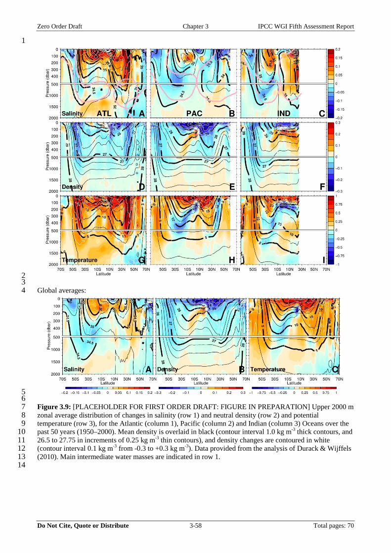
Zero Order Draft Chapter 3 IPCC WGI Fifth Assessment Report
Do Not Cite, Quote or Distribute 3-58 Total pages: 70
1
2 3 Global averages: 4
5 6 Figure 3.9: [PLACEHOLDER FOR FIRST ORDER DRAFT: FIGURE IN PREPARATION] Upper 2000 m 7 zonal average distribution of changes in salinity (row 1) and neutral density (row 2) and potential 8 temperature (row 3), for the Atlantic (column 1), Pacific (column 2) and Indian (column 3) Oceans over the 9 past 50 years (1950–2000). Mean density is overlaid in black (contour interval 1.0 kg m-3 thick contours, and 10 26.5 to 27.75 in increments of 0.25 kg m-3 thin contours), and density changes are contoured in white 11 (contour interval 0.1 kg m-3 from -0.3 to +0.3 kg m-3). Data provided from the analysis of Durack & Wijffels 12 (2010). Main intermediate water masses are indicated in row 1. 13
14

Zero Order Draft Chapter 3 IPCC WGI Fifth Assessment Report
Do Not Cite, Quote or Distribute 3-59 Total pages: 70
1
2 3 Figure 3.10: The mean SSH (cm, black contours) for the Argo era is the sum of the geostrophic pressure 4 field at 1000 m based on Argo trajectory data (Katsumata and Yoshinari, 2010) plus the relative pressure 5 field (0/1000 dbar steric height) based on Argo profile data from Roemmich and Gilson (2009). The SSH 6 difference (cm, color shading) between the Argo era (2004–2009) and the first decade of altimetry (1993–7 2002) is based on the AVISO altimetry “reference” product (Ducet et al, 2000). 8
9

Zero Order Draft Chapter 3 IPCC WGI Fifth Assessment Report
Do Not Cite, Quote or Distribute 3-60 Total pages: 70
1
2 3 Figure 3.11: [PLACEHOLDER FOR FIRST ORDER DRAFT: final figure will include time series from 4 RAPID and MOVE array] Merged time series of Atlantic MOC transport based on 3 different estimates: (i) 5 Rapid/MOCHA array at 26°N from 2004 to present, (ii) Willis (2010) estimate at 41°N based on 6 Argo+altimetry, 2002 to present, and from altimetry alone, 1993–2001, (iii) Grist et al. (2009) estimate based 7 on surface thermohaline forcing. 8
9

Zero Order Draft Chapter 3 IPCC WGI Fifth Assessment Report
Do Not Cite, Quote or Distribute 3-61 Total pages: 70
a) 1
2 3 b) 4
5 6 Figure 3.12: Global mean sea level from a) tide gauges (1870–2007), updated from Church and White 7 (2006) and Jevrejeva et al. (2006) and b) altimetry (1993–2010) updated from Nerem et al. (2010), GRACE 8 (2003–2010) updated from Chambers et al. (2010), and thermosteric (1993–2005) updated from Domingues 9 et al. (2008). The Church and White (2006) data are yearly averages, while the Jevrejeva et al. (2006) data 10 are monthly values integrated from low-pass filtered weighted-average annual trends of sea level. The 11 altimetry, GRACE, and thermosteric data have been smoothed with a 6-month running mean filter. All 12 uncertainty bars are 1-standard error. The tide gauge records are plotted relative to a mean in 1900; the 13 altimeter, thermosteric, and GRACE are plotted relative to a mean in 2003. 14
15

Zero Order Draft Chapter 3 IPCC WGI Fifth Assessment Report
Do Not Cite, Quote or Distribute 3-62 Total pages: 70
1 2 3 Figure 3.13: [PLACEHOLDER FOR FIRST ORDER DRAFT: Caption still needs to be written and Figure 4 needs to be made.] Global map of trends in SWH from one source. 5
6

Zero Order Draft Chapter 3 IPCC WGI Fifth Assessment Report
Do Not Cite, Quote or Distribute 3-63 Total pages: 70
1
2 3 Figure 3.14: Compilation of 2008 column inventories (mol m-2) of anthropogenic CO2: the global Ocean 4 excluding the marginal seas (Khatiwala et al., 2009) 140 ± 25 PgC; Arctic Ocean (Tanhua et al 2009) 2.6–5 3.4 PgC; the Nordic Seas (Olsen et al 2010) 1.0–1.5 PgC; the Mediterranean Sea (Schneider et al., 2010) 6 1.5–2.4 PgC; the East Sea (Sea of Japan) (Park et al 2006) 0.40 ± 0.06 Pg C. 7
8
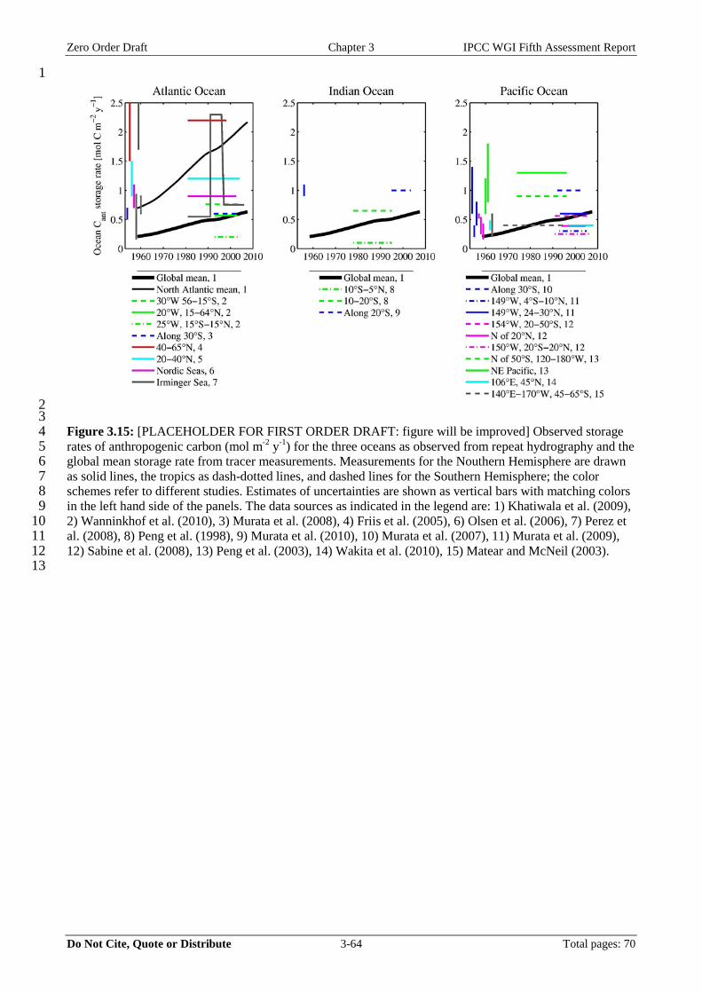
Zero Order Draft Chapter 3 IPCC WGI Fifth Assessment Report
Do Not Cite, Quote or Distribute 3-64 Total pages: 70
1
2 3 Figure 3.15: [PLACEHOLDER FOR FIRST ORDER DRAFT: figure will be improved] Observed storage 4 rates of anthropogenic carbon (mol m-2 y-1) for the three oceans as observed from repeat hydrography and the 5 global mean storage rate from tracer measurements. Measurements for the Nouthern Hemisphere are drawn 6 as solid lines, the tropics as dash-dotted lines, and dashed lines for the Southern Hemisphere; the color 7 schemes refer to different studies. Estimates of uncertainties are shown as vertical bars with matching colors 8 in the left hand side of the panels. The data sources as indicated in the legend are: 1) Khatiwala et al. (2009), 9 2) Wanninkhof et al. (2010), 3) Murata et al. (2008), 4) Friis et al. (2005), 6) Olsen et al. (2006), 7) Perez et 10 al. (2008), 8) Peng et al. (1998), 9) Murata et al. (2010), 10) Murata et al. (2007), 11) Murata et al. (2009), 11 12) Sabine et al. (2008), 13) Peng et al. (2003), 14) Wakita et al. (2010), 15) Matear and McNeil (2003). 12
13
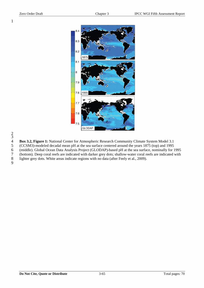
Zero Order Draft Chapter 3 IPCC WGI Fifth Assessment Report
Do Not Cite, Quote or Distribute 3-65 Total pages: 70
1
2 3 Box 3.2, Figure 1: National Center for Atmospheric Research Community Climate System Model 3.1 4 (CCSM3)-modeled decadal mean pH at the sea surface centered around the years 1875 (top) and 1995 5 (middle). Global Ocean Data Analysis Project (GLODAP)-based pH at the sea surface, nominally for 1995 6 (bottom). Deep coral reefs are indicated with darker grey dots; shallow-water coral reefs are indicated with 7 lighter grey dots. White areas indicate regions with no data (after Feely et al., 2009). 8
9

Zero Order Draft Chapter 3 IPCC WGI Fifth Assessment Report
Do Not Cite, Quote or Distribute 3-66 Total pages: 70
1
2 3 Box 3.2, Figure 2: [PLACEHOLDER FOR FIRST ORDER DRAFT: figure will be improved] Distribution 4 of: a) pH and b) CO3
2– concentration in the Pacific, Atlantic, and Indian oceans. The data are from the World 5 Ocean Circulation Experiment/Joint Global Ocean Flux Study/Ocean Atmosphere Carbon Exchange Study 6 global CO2 survey (Sabine et al., 2005). The lines show the average aragonite (solid line) and calcite (dashed 7 line) saturation CO3
2– concentration for each of these basins. The color coding shows the latitude bands for 8 the data sets (after Feely et al., 2009). 9
10

Zero Order Draft Chapter 3 IPCC WGI Fifth Assessment Report
Do Not Cite, Quote or Distribute 3-67 Total pages: 70
1
2 3 Figure 3.16: Long-term trends of surface seawater pCO2 (top), pH (middle), and carbonate ion (bottom) 4 concentration at three subtropical ocean time series in the North Atlantic and North Pacific Oceans, 5 including: (1) Bermuda Atlantic Time Series Study (BATS, 31°40′N, 64°10′W; green line) and Hydrostation 6 S (32°10′, 64°30′W) from 1983 to present (Bates, 2007); (2) Hawaii Ocean Time Series (HOT) at Station 7 ALOHA (A Long-term Oligotrophic Habitat Assessment; 22°45′N, 158°00′W; orange line) from 1988 to 8 present (Dore et al., 2009), and; (3) European Station for Time Series in the Ocean (ESTOC, 29°10′N, 9 15°30′W; blue line) from 1994 to present (González-Dávila et al., 2010). Atmospheric pCO2 (black line) 10 from Hawaii is shown in the top panel. 11
12

Zero Order Draft Chapter 3 IPCC WGI Fifth Assessment Report
Do Not Cite, Quote or Distribute 3-68 Total pages: 70
1
2 3 Figure 3.17: ΔpHant: pH change attributed to the uptake of anthropogenic carbon between 1991 and 2006 4 (from Byrne et al., 2010). 5
6

Zero Order Draft Chapter 3 IPCC WGI Fifth Assessment Report
Do Not Cite, Quote or Distribute 3-69 Total pages: 70
1 2 Figure 3.18: Long-term evolution of oxygen in 4 representative locations in the tropical ocean: A and C, 3 tropical Atlantic; D and E, Tropical Pacific (adapted from Stramma et al., 2008). 4
5

Zero Order Draft Chapter 3 IPCC WGI Fifth Assessment Report
Do Not Cite, Quote or Distribute 3-70 Total pages: 70
1
2 3 FAQ 3.1, Figure 1: Ocean warming pathways. The ocean is stratified, with the coldest water, Antarctic 4 Bottom Water (dark blue) sinking around Antarctica and spreading northward along the ocean floor into the 5 central Pacific (bottom panel, left) and western Atlantic (bottom panel, right) oceans, as well as the Indian 6 Ocean (not shown). North Atlantic Deep Water (lighter blue) sinks in the northern North Atlantic Ocean and 7 spreads south above the Antarctic Bottom Water and then around Antarctica and into the Pacific and Indian 8 Oceans. Similarly, in the upper ocean (top left panel) Intermediate Waters (cyan) sink in subpolar regions 9 and slip equatorward under Subtropical Waters (green), which in turn slip equatorward under tropical waters 10 (orange) in all three oceans. Excess heat entering at the ocean surface also mixes slowly downward (squiggly 11 red arrows). 12