chapter 3 mobile combustion - institute for global ... · 3.5.1.4 military ... table 3.4.1 default...
TRANSCRIPT

Chapter 3: Mobile Combustion
2006 IPCC Guidelines for National Greenhouse Gas Inventories 3.1
C H A P T E R 3
MOBILE COMBUSTION

Volume 2: Energy
3.2 2006 IPCC Guidelines for National Greenhouse Gas Inventories
Authors
Overview
Christina Davies Waldron (USA)
Jochen Harnisch (Germany), Oswaldo Lucon (Brazil), R. Scott Mckibbon (Canada), Sharon B. Saile (USA), Fabian Wagner (Germany), and Michael P. Walsh (USA)
Off-road transportat ion
Christina Davies Waldron (USA)
Jochen Harnisch (Germany), Oswaldo Lucon (Brazil), R. Scott McKibbon (Canada), Sharon Saile (USA), Fabian Wagner (Germany), and Michael Walsh (USA)
Railways
Christina Davies Waldron (USA)
Jochen Harnisch (Germany), Oswaldo Lucon (Brazil), R. Scott McKibbon (Canada), Sharon B. Saile (USA), Fabian Wagner (Germany), and Michael P. Walsh (USA)
Water-borne navigat ion
Lourdes Q. Maurice (USA)
Leif Hockstad (USA), Niklas Höhne (Germany), Jane Hupe (ICAO), David S. Lee (UK), and Kristin Rypdal (Norway)
Civi l aviat ion
Lourdes Q. Maurice (USA)
Leif Hockstad (USA), Niklas Höhne (Germany), Jane Hupe (ICAO), David S. Lee (UK), and Kristin Rypdal (Norway)
Contributing Authors
Road transportat ion, Off-road transportat ion and Railways
Manmohan Kapshe (India)
Water-borne navigat ion and Civi l Aviat ion
Daniel M. Allyn (USA), Maryalice Locke (USA, Stephen Lukachko (USA), and Stylianos Pesmajoglou (UNFCCC)

Chapter 3: Mobile Combustion
2006 IPCC Guidelines for National Greenhouse Gas Inventories 3.3
Contents
3 Mobile Combustion
3.1 Overview...............................................................................................................................................3.8 3.2 Road Transportation............................................................................................................................3.10
3.2.1 Methodological issues .................................................................................................................3.10 3.2.1.1 Choice of method...................................................................................................................3.10 3.2.1.2 Choice of emission factors.....................................................................................................3.16 3.2.1.3 Choice of activity data ...........................................................................................................3.25 3.2.1.4 Completeness.........................................................................................................................3.28 3.2.1.5 Developing a consistent time series .......................................................................................3.29
3.2.2 Uncertainty assessment ...............................................................................................................3.29 3.2.3 Inventory Quality Assurance/Quality Control (QA/QC).............................................................3.31 3.2.4 Reporting and Documentation.....................................................................................................3.32 3.2.5 Reporting tables and worksheets .................................................................................................3.32
3.3 Off-road Transportation ......................................................................................................................3.32 3.3.1 Methodological issues .................................................................................................................3.32
3.3.1.1 Choice of method...................................................................................................................3.32 3.3.1.2 Choice of emission factors.....................................................................................................3.35 3.3.1.3 Choice of activity data ...........................................................................................................3.36 3.3.1.4 Completeness.........................................................................................................................3.37 3.3.1.5 Developing a consistent time series .......................................................................................3.37
3.3.2 Uncertainty assessment ...............................................................................................................3.38 3.3.2.1 Activity data uncertainty........................................................................................................3.38
3.3.3 Inventory Quality Assurance/Quality Control (QA/QC).............................................................3.38 3.3.4 Reporting and Documentation.....................................................................................................3.39 3.3.5 Reporting tables and worksheets .................................................................................................3.39
3.4 Railways..............................................................................................................................................3.39 3.4.1 Methodological issues .................................................................................................................3.40
3.4.1.1 Choice of method...................................................................................................................3.40 3.4.1.2 Choice of emission factors.....................................................................................................3.42 3.4.1.3 Choice of activity data ...........................................................................................................3.44 3.4.1.4 Completeness.........................................................................................................................3.45 3.4.1.5 Developing a consistent time series .......................................................................................3.45 3.4.1.6 Uncertainty assessment..........................................................................................................3.45
3.4.2 Inventory Quality Assurance/Quality Control (QA/QC).............................................................3.46 3.4.3 Reporting and Documentation.....................................................................................................3.46 3.4.4 Reporting tables and worksheets .................................................................................................3.47
3.5 Water-borne Navigation......................................................................................................................3.47

Volume 2: Energy
3.4 2006 IPCC Guidelines for National Greenhouse Gas Inventories
3.5.1 Methodological issues .................................................................................................................3.47 3.5.1.1 Choice of method...................................................................................................................3.47 3.5.1.2 Choice of emission factors.....................................................................................................3.50 3.5.1.3 Choice of activity data ...........................................................................................................3.51 3.5.1.4 Military ..................................................................................................................................3.53 3.5.1.5 Completeness.........................................................................................................................3.53 3.5.1.6 Developing a consistent time series .......................................................................................3.53 3.5.1.7 Uncertainty assessment..........................................................................................................3.54
3.5.2 Inventory Quality Assurance/Quality Control (QA/QC).............................................................3.54 3.5.3 Reporting and Documentation.....................................................................................................3.55 3.5.4 Reporting tables and worksheets .................................................................................................3.55 3.5.5 Definitions of specialist terms .....................................................................................................3.56
3.6 Civil Aviation......................................................................................................................................3.56 3.6.1 Methodological issues .................................................................................................................3.57
3.6.1.1 Choice of method...................................................................................................................3.57 3.6.1.2 Choice of emission factors.....................................................................................................3.64 3.6.1.3 Choice of activity data ...........................................................................................................3.65 3.6.1.4 Military aviation ....................................................................................................................3.66 3.6.1.5 Completeness.........................................................................................................................3.68 3.6.1.6 Developing a consistent time series .......................................................................................3.68 3.6.1.7 Uncertainty assessment..........................................................................................................3.69
3.6.2 Inventory Quality Assurance/Quality Control (QA/QC).............................................................3.69 3.6.3 Reporting and Documentation.....................................................................................................3.73 3.6.4 Reporting tables and worksheets .................................................................................................3.73 3.6.5 Definitions of specialist terms .....................................................................................................3.74
References .....................................................................................................................................................3.74

Chapter 3: Mobile Combustion
2006 IPCC Guidelines for National Greenhouse Gas Inventories 3.5
Equations
Equation 3.2.1 CO2 from road transport ...................................................................................................3.12
Equation 3.2.2 CO2 from urea-based catalytic converters ...........................................................................3.12 Equation 3.2.3 Tier 1 emissions of CH4 and N2O........................................................................................3.13 Equation 3.2.4 Tier 2 emissions of CH4 and N2O........................................................................................3.13 Equation 3.2.5 Tier 3 emissions of CH4 and N2O........................................................................................3.15 Equation 3.2.6 Validating fuel consumption ...............................................................................................3.26 Equation 3.3.1 Tier 1 emissions estimate ....................................................................................................3.33 Equation 3.3.2 Tier 2 emissions estimate ....................................................................................................3.33 Equation 3.3.3 Tier 3 emissions estimate ....................................................................................................3.34 Equation 3.3.4 Emissions from urea-based catalytic converters..................................................................3.35 Equation 3.4.1 General method for emissions from locomotives ................................................................3.41 Equation 3.4.2 Tier 2 method for CH4 and N2O from locomotives .............................................................3.42 Equation 3.4.3 Tier 3 example of a method for CH4 and N2O from locomotives........................................3.42 Equation 3.4.4 Weighting of CH4 and N2O emission factors for specific technologies ..............................3.43 Equation 3.4.5 Estimating yard locomotive fuel consumption ....................................................................3.45 Equation 3.5.1 Water-borne navigation equation ........................................................................................3.47 Equation 3.6.1 (Aviation equation 1)...........................................................................................................3.59 Equation 3.6.2 (Aviation equation 2)...........................................................................................................3.59 Equation 3.6.3 (Aviation equation 3)...........................................................................................................3.59 Equation 3.6.4 (Aviation equation 4)...........................................................................................................3.59 Equation 3.6.5 (Aviation equation 5)...........................................................................................................3.59
Figures
Figure 3.2.1 Steps in estimating emissions from road transport ..............................................................3.11 Figure 3.2.2 Decision tree for CO2 emissions from fuel combustion in road vehicles ............................3.11 Figure 3.2.3 Decision tree for CH4 and N2O emissions from road vehicles ............................................3.14 Figure 3.3.1 Decision tree for estimating emissions from off-road vehicles ...........................................3.34 Figure 3.4.1 Decision tree for estimating CO2 emissions from railways .................................................3.40 Figure 3.4.2 Decision tree for estimating CH4 and N2O emissions from railways ..................................3.41 Figure 3.5.1 Decision tree for emissions from water-borne navigation...................................................3.49 Figure 3.6.1 Decision tree for estimating aircraft emissions (applied to each greenhouse gas)...............3.60 Figure 3.6.2 Estimating aircraft emissions with Tier 2 method ...............................................................3.62

Volume 2: Energy
3.6 2006 IPCC Guidelines for National Greenhouse Gas Inventories
Tables
Table 3.1.1 Detailed sector split for the transport sector ..........................................................................3.8
Table 3.2.1 Road transport default CO2 emission factors and uncertainty ranges..................................3.16
Table 3.2.2 Road transport N2O and CH4 default emission factors and uncertainty ranges ...................3.21
Table 3.2.3 N2O and CH4 emission factors for USA gasoline and diesel vehicles.................................3.22
Table 3.2.4 Emission factors for alternative fuel vehicles......................................................................3.23
Table 3.2.5 Emission factors for European gasoline and diesel vehicles, COPERT IV model ..............3.24
Table 3.3.1 Default emission factors for off-road mobile sources and machinery .................................3.36
Table 3.4.1 Default emission factors for the most common fuels used for rail transport .......................3.43
Table 3.4.2 Pollutant weghting factors as functions of engine design parameters for uncontrolled engines(dimensionless)...................................................................................3.43
Table 3.5.1 Source category structure ....................................................................................................3.48
Table 3.5.2 CO2 emission factors ...........................................................................................................3.50
Table 3.5.3 Default water-borne navigation CH4 and N2O emission factors..........................................3.50
Table 3.5.4 Criteria for defining international or domestic water-borne navigation (applies to each segment of a voyage calling at more than two ports) ................................3.51
Table 3.5.5 Average fuel consumption per engine type (ships >500 GRT) ...........................................3.52
Table 3.5.6 Fuel consumption factors, full power ..................................................................................3.52
Table 3.6.1 Source categories.................................................................................................................3.58
Table 3.6.2 Data requirements for different tiers....................................................................................3.58
Table 3.6.3 Correspondence between representative aircraft and other aircraft types............................3.63
Table 3.6.4 CO2 emission factors ...........................................................................................................3.64
Table 3.6.5 Non-CO2 emission factors ...................................................................................................3.64
Table 3.6.6 Criteria for defining international or domestic aviation (applies to individual legs of journeys with more than one take-off and landing) ................................................3.65
Table 3.6.7 Fuel consumption factors for military aircraft .....................................................................3.67
Table 3.6.8 Fuel consumption per flight hour for military aircraft.........................................................3.67
Table 3.6.9 LTO emission factors for typical aircraft ............................................................................3.70
Table 3.6.10 NOx emission factors for various aircraft at cruise levels....................................................3.72

Chapter 3: Mobile Combustion
2006 IPCC Guidelines for National Greenhouse Gas Inventories 3.7
Boxes
Box 3.2.1 Examples of biofuel use in road transportation ...................................................................3.18
Box 3.2.2 Refining emission factors for mobile sources in developing countries ...............................3.20
Box 3.2.3 Vehicle deterioration (scrappage) curves ............................................................................3.28
Box 3.2.4 Lubricants in mobile combustion ........................................................................................3.29
Box 3.3.1 Nonroad emission model (USEPA).....................................................................................3.37
Box 3.3.2 Canadian experience with nonroad model...........................................................................3.38
Box 3.4.1 Example of Tier 3 approach ................................................................................................3.44

Volume 2: Energy
3.8 2006 IPCC Guidelines for National Greenhouse Gas Inventories
3 MOBILE COMBUSTION
3.1 OVERVIEW Mobile sources produce direct greenhouse gas emissions of carbon dioxide (CO2), methane (CH4) and nitrous oxide (N2O) from the combustion of various fuel types, as well as several other pollutants such as carbon monoxide (CO), Non-methane Volatile Organic Compounds (NMVOCs), sulphur dioxide (SO2), particulate matter (PM) and oxides of nitrate (NOx), which cause or contribute to local or regional air pollution. This chapter covers good practice in the development of estimates for the direct greenhouse gases CO2, CH4, and N2O. For indirect greenhouse gases and precursor substances CO, NMVOCs, SO2, PM, and NOx, please refer to Volume 1 Chapter 7. This chapter does not address non-energy emissions from mobile air conditioning, which is covered by the IPPU Volume (Volume 3, Chapter 7).
Greenhouse gas emissions from mobile combustion are most easily estimated by major transport activity, i.e., road, off-road, air, railways, and water-borne navigation. The source description (Table 3.1.1) shows the diversity of mobile sources and the range of characteristics that affect emission factors. Recent work has updated and strengthened the data. Despite these advances more work is needed to fill in many gaps in knowledge of emissions from certain vehicle types and on the effects of ageing on catalytic control of road vehicle emissions. Equally, the information on the appropriate emission factors for road transport in developing countries may need further strengthening, where age of fleet, maintenance, fuel sulphur content, and patterns of use are different from those in industrialised countries.
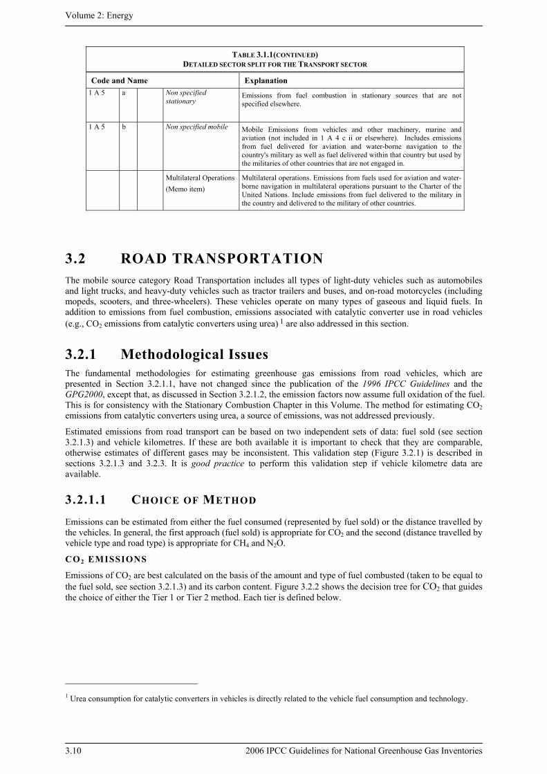
TABLE 3.1.1 DETAILED SECTOR SPLIT FOR THE TRANSPORT SECTOR
Code and Name Explanation 1 A 3 TRANSPORT Emissions from the combustion and evaporation of fuel for all transport
activity (excluding military transport), regardless of the sector, specified by sub-categories below. Emissions from fuel sold to any air or marine vessel engaged in international transport (1 A 3 a i and 1 A 3 d i) should as far as possible be excluded from the totals and subtotals in this category and should be reported separately.
1 A 3 a Civil Aviation Emissions from international and domestic civil aviation, including take-offs and landings. Comprises civil commercial use of airplanes, including: scheduled and charter traffic for passengers and freight, air taxiing, and general aviation. The international/domestic split should be determined on the basis of departure and landing locations for each flight stage and not by the nationality of the airline. Exclude use of fuel at airports for ground transport which is reported under 1 A 3 e Other Transportation. Also exclude fuel for stationary combustion at airports; report this information under the appropriate stationary combustion category.
1 A 3 a i International Aviation (International Bunkers)
Emissions from flights that depart in one country and arrive in a different country. Include take-offs and landings for these flight stages. Emissions from international military aviation can be included as a separate sub-category of international aviation provided that the same definitional distinction is applied and data are available to support the definition.
1 A 3 a ii Domestic Aviation Emissions from civil domestic passenger and freight traffic that departs and arrives in the same country (commercial, private, agriculture, etc.), including take-offs and landings for these flight stages. Note that this may include journeys of considerable length between two airports in a country (e.g. San Francisco to Honolulu). Exclude military, which should be reported under 1 A 5 b.
1 A 3 b Road Transportation All combustion and evaporative emissions arising from fuel use in road vehicles, including the use of agricultural vehicles on paved roads.
1 A 3 b i Cars Emissions from automobiles so designated in the vehicle registering country primarily for transport of persons and normally having a capacity of 12 persons or fewer.
1 A 3 b i 1 Passenger cars with 3-way catalysts
Emissions from passenger car vehicles with 3-way catalysts.
1 A 3 b i 2 Passenger cars without 3-way catalysts
Emissions from passenger car vehicles without 3-way catalysts.

Chapter 3: Mobile Combustion
2006 IPCC Guidelines for National Greenhouse Gas Inventories 3.9
TABLE 3.1.1(CONTINUED) DETAILED SECTOR SPLIT FOR THE TRANSPORT SECTOR
Code and Name Explanation 1 A 3 b ii Light duty trucks Emissions from vehicles so designated in the vehicle registering country
primarily for transportation of light-weight cargo or which are equipped with special features such as four-wheel drive for off-road operation. The gross vehicle weight normally ranges up to 3500-3900 kg or less.
1 A 3 b ii 1 Light duty trucks with 3-way catalysts
Emissions from light duty trucks with 3-way catalysts.
1 A 3 b ii 2 Light duty trucks without 3-way catalysts
Emissions from light duty trucks without 3-way catalysts.
1 A 3 b iii Heavy duty trucks and buses
Emissions from any vehicles so designated in the vehicle registering country. Normally the gross vehicle weight ranges from 3500-3900 kg or more for heavy duty trucks and the buses are rated to carry more than 12 persons.
1 A 3 b iv Motorcycles Emissions from any motor vehicle designed to travel with not more than three wheels in contact with the ground and weighing less than 680 kg.
1 A 3 b v Evaporative emissions from vehicles
Evaporative emissions from vehicles (e.g. hot soak, running losses) are included here. Emissions from loading fuel into vehicles are excluded.
1 A 3 b vi Urea-based catalysts CO2 emissions from use of urea-based additives in catalytic converters (non-combustive emissions)
1 A 3 c Railways Emissions from railway transport for both freight and passenger traffic routes.
1 A 3 d Water-borne Navigation Emissions from fuels used to propel water-borne vessels, including hovercraft and hydrofoils, but excluding fishing vessels. The international/domestic split should be determined on the basis of port of departure and port of arrival, and not by the flag or nationality of the ship.
1 A 3 d i International water-borne navigation (International bunkers)
Emissions from fuels used by vessels of all flags that are engaged in international water-borne navigation. The international navigation may take place at sea, on inland lakes and waterways and in coastal waters. Includes emissions from journeys that depart in one country and arrive in a different country. Exclude consumption by fishing vessels (see Other Sector - Fishing). Emissions from international military water-borne navigation can be included as a separate sub-category of international water-borne navigation provided that the same definitional distinction is applied and data are available to support the definition.
1 A 3 d ii Domestic water-borne Navigation
Emissions from fuels used by vessels of all flags that depart and arrive in the same country (exclude fishing, which should be reported under 1 A 4 c iii, and military, which should be reported under 1 A 5 b). Note that this may include journeys of considerable length between two ports in a country (e.g. San Francisco to Honolulu).
1 A 3 e Other Transportation Combustion emissions from all remaining transport activities including pipeline transportation, ground activities in airports and harbours, and off-road activities not otherwise reported under 1 A 4 c Agriculture or 1 A 2. Manufacturing Industries and Construction. Military transport should be reported under 1 A 5 (see 1 A 5 Non-specified).
1 A 3 e i Pipeline Transport Combustion related emissions from the operation of pump stations and maintenance of pipelines. Transport via pipelines includes transport of gases, liquids, slurry and other commodities via pipelines. Distribution of natural or manufactured gas, water or steam from the distributor to final users is excluded and should be reported in 1 A 1 c ii or 1 A 4 a.
1 A 3 e ii Off-road Combustion emissions from Other Transportation excluding Pipeline Transport.
1 A 4 c iii Fishing (mobile combustion)
Emissions from fuels combusted for inland, coastal and deep-sea fishing. Fishing should cover vessels of all flags that have refuelled in the country (include international fishing).
Volume 2: Energy
3.10 2006 IPCC Guidelines for National Greenhouse Gas Inventories
TABLE 3.1.1(CONTINUED) DETAILED SECTOR SPLIT FOR THE TRANSPORT SECTOR
Code and Name Explanation 1 A 5 a Non specified
stationary Emissions from fuel combustion in stationary sources that are not specified elsewhere.
1 A 5 b Non specified mobile Mobile Emissions from vehicles and other machinery, marine and aviation (not included in 1 A 4 c ii or elsewhere). Includes emissions from fuel delivered for aviation and water-borne navigation to the country's military as well as fuel delivered within that country but used by the militaries of other countries that are not engaged in.
Multilateral Operations (Memo item)
Multilateral operations. Emissions from fuels used for aviation and water-borne navigation in multilateral operations pursuant to the Charter of the United Nations. Include emissions from fuel delivered to the military in the country and delivered to the military of other countries.
3.2 ROAD TRANSPORTATION The mobile source category Road Transportation includes all types of light-duty vehicles such as automobiles and light trucks, and heavy-duty vehicles such as tractor trailers and buses, and on-road motorcycles (including mopeds, scooters, and three-wheelers). These vehicles operate on many types of gaseous and liquid fuels. In addition to emissions from fuel combustion, emissions associated with catalytic converter use in road vehicles (e.g., CO2 emissions from catalytic converters using urea) 1 are also addressed in this section.
3.2.1 Methodological Issues The fundamental methodologies for estimating greenhouse gas emissions from road vehicles, which are presented in Section 3.2.1.1, have not changed since the publication of the 1996 IPCC Guidelines and the GPG2000, except that, as discussed in Section 3.2.1.2, the emission factors now assume full oxidation of the fuel. This is for consistency with the Stationary Combustion Chapter in this Volume. The method for estimating CO2 emissions from catalytic converters using urea, a source of emissions, was not addressed previously.
Estimated emissions from road transport can be based on two independent sets of data: fuel sold (see section 3.2.1.3) and vehicle kilometres. If these are both available it is important to check that they are comparable, otherwise estimates of different gases may be inconsistent. This validation step (Figure 3.2.1) is described in sections 3.2.1.3 and 3.2.3. It is good practice to perform this validation step if vehicle kilometre data are available.
3.2.1.1 CHOICE OF METHOD Emissions can be estimated from either the fuel consumed (represented by fuel sold) or the distance travelled by the vehicles. In general, the first approach (fuel sold) is appropriate for CO2 and the second (distance travelled by vehicle type and road type) is appropriate for CH4 and N2O.
CO2 EMISSIONS
Emissions of CO2 are best calculated on the basis of the amount and type of fuel combusted (taken to be equal to the fuel sold, see section 3.2.1.3) and its carbon content. Figure 3.2.2 shows the decision tree for CO2 that guides the choice of either the Tier 1 or Tier 2 method. Each tier is defined below.
1 Urea consumption for catalytic converters in vehicles is directly related to the vehicle fuel consumption and technology.

Chapter 3: Mobile Combustion
2006 IPCC Guidelines for National Greenhouse Gas Inventories 3.11
Figure 3.2.1 Steps in estimating emissions from road transport
Start
Estimate CH4 and N2O.(see decision tree)
Validate fuel statistics andvehicle kilometre data and
correct if necessary.
Estimate CO2.(see decision tree)
Figure 3.2.2 Decision tree for CO2 emissions from fuel combustion in road vehicles
Start
Arecountry-specific
fuel carbon contentsavailable?
Is this a keycategory?
Use country-specificcarbon contents.
Yes
Yes
No
No
Collect country-specific carbon.
Use defaultcarbon contents.
Box 2: Tier 1
Box 1: Tier 2
Note: See Volume 1 Chapter 4, “Methodological Choice and Key Categories” (noting section 4.1.2 on limited resources) for discussion of key categories and use of decision trees.

Volume 2: Energy
3.12 2006 IPCC Guidelines for National Greenhouse Gas Inventories
The Tier 1 approach calculates CO2 emissions by multiplying estimated fuel sold with a default CO2 emission factor. The approach is represented in Equation 3.2.1.
EQUATION 3.2.1 CO2 FROM ROAD TRANSPORT
]FE[FuelEmission aa
a∑ •=
Where:
Emission = Emissions of CO2 (kg)
Fuela = fuel sold (TJ)
EFa = emission factor (kg/TJ). This is equal to the carbon content of the fuel multiplied by 44/12.
a = type of fuel (e.g. petrol, diesel, natural gas, LPG etc)
The CO2 emission factor takes account of all the carbon in the fuel including that emitted as CO2, CH4, CO, NMVOC and particulate matter2 . Any carbon in the fuel derived from biomass should be reported as an information item and not included in the sectoral or national totals to avoid double counting as the net emissions from biomass are already accounted for in the AFOLU sector (see section 3.2.1.4 Completeness).
The Tier 2 approach is the same as Tier 1 except that country-specific carbon contents of the fuel sold in road transport are used. Equation 3.2.1 still applies but the emission factor is based on the actual carbon content of fuels consumed (as represented by fuel sold) in the country during the inventory year. At Tier 2, the CO2 emission factors may be adjusted to take account of un-oxidised carbon or carbon emitted as a non-CO2 gas.
There is no Tier 3 as it is not possible to produce significantly better results for CO2 than by using the existing Tier 2. In order to reduce the uncertainties, efforts should concentrate on the carbon content and on improving the data on fuel sold. Another major uncertainty component is the use of transport fuel for non-road purposes.
CO2 EMISSIONS FROM UREA-BASED CATALYSTS
For estimating CO2 emissions from use of urea-based additives in catalytic converters (non-combustive emissions), it is good practice to use Equation 3.2.2:
EQUATION 3.2.2 CO2 FROM UREA-BASED CATALYTIC CONVERTERS
1244
6012
•••= PurityActivityEmission
Where:
Emissions = CO2 Emissions from urea-based additive in catalytic converters (Gg CO2) Activity = amount of urea-based additive consumed for use in catalytic converters (Gg) Purity = the mass fraction (= percentage divided by 100) of urea in the urea-based additive
The factor (12/60) captures the stochiometric conversion from urea (CO(NH2)2) to carbon, while factor (44/12) converts carbon to CO2. On the average, the activity level is 1 to 3 percent of diesel consumption by the vehicle. Thirty two and half percent can be taken as default purity in case country-specific values are not available (Peckham, 2003). As this is based on the properties of the materials used, there are no tiers for this source.
CH4 AND N2O EMISSIONS
Emissions of CH4 and N2O are more difficult to estimate accurately than those for CO2 because emission factors depend on vehicle technology, fuel and operating characteristics. Both distance-based activity data (e.g. vehicle-kilometres travelled) and disaggregated fuel consumption may be considerably less certain than overall fuel sold.
CH4 and N2O emissions are significantly affected by the distribution of emission controls in the fleet. Thus higher tiers use an approach taking into account populations of different vehicle types and their different pollution control technologies.
2 Research on carbon mass balances for U.S. light-duty gasoline cars and trucks indicates that “the fraction of solid
(unoxidized) carbon is negligible” USEPA (2004a). This did not address two-stroke engines or fuel types other than gasoline. Additional discussion of the 100 percent oxidation assumption is included in Section 1.4.2.1 of the Energy Volume Introduction chapter.
Chapter 3: Mobile Combustion
2006 IPCC Guidelines for National Greenhouse Gas Inventories 3.13
Although CO2 emissions from biogenic carbon are not included in national totals, the combustion of biofuels in mobile sources generates anthropogenic CH4 and N2O that should be calculated and reported in emissions estimates.
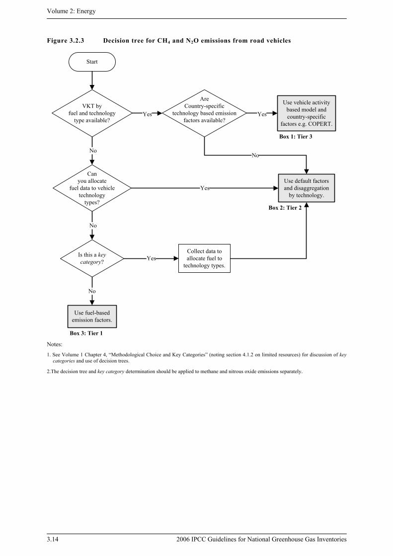
The decision tree in Figure 3.2.3 outlines choice of method for calculating emissions of CH4 and N2O. The inventory compiler should choose the method on the basis of the existence and quality of data. The tiers are defined in the corresponding equations 3.2.3 to 3.2.5, below.
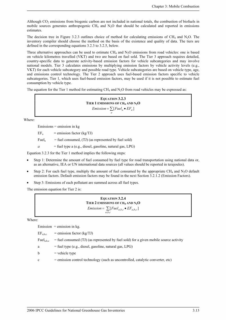
Three alternative approaches can be used to estimate CH4 and N2O emissions from road vehicles: one is based on vehicle kilometres travelled (VKT) and two are based on fuel sold. The Tier 3 approach requires detailed, country-specific data to generate activity-based emission factors for vehicle subcategories and may involve national models. Tier 3 calculates emissions by multiplying emission factors by vehicle activity levels (e.g., VKT) for each vehicle subcategory and possible road type. Vehicle subcategories are based on vehicle type, age, and emissions control technology. The Tier 2 approach uses fuel-based emission factors specific to vehicle subcategories. Tier 1, which uses fuel-based emission factors, may be used if it is not possible to estimate fuel consumption by vehicle type.
The equation for the Tier 1 method for estimating CH4 and N2O from road vehicles may be expressed as:
EQUATION 3.2.3 TIER 1 EMISSIONS OF CH4 AND N2O
∑ •=a
aa EFFuelEmission ][
Where:
Emissions = emission in kg
EFa = emission factor (kg/TJ)
Fuela = fuel consumed, (TJ) (as represented by fuel sold)
a = fuel type a (e.g., diesel, gasoline, natural gas, LPG)
Equation 3.2.3 for the Tier 1 method implies the following steps:
• Step 1: Determine the amount of fuel consumed by fuel type for road transportation using national data or, as an alternative, IEA or UN international data sources (all values should be reported in terajoules).
• Step 2: For each fuel type, multiply the amount of fuel consumed by the appropriate CH4 and N2O default emission factors. Default emission factors may be found in the next Section 3.2.1.2 (Emission Factors).
• Step 3: Emissions of each pollutant are summed across all fuel types.
The emission equation for Tier 2 is:
EQUATION 3.2.4 TIER 2 EMISSIONS OF CH4 AND N2O
][,,
,,,,∑ •=cba
cbacba EFFuelEmission
Where:
Emission = emission in kg.
EFa,b,c = emission factor (kg/TJ)
Fuela,b,c = fuel consumed (TJ) (as represented by fuel sold) for a given mobile source activity
a = fuel type (e.g., diesel, gasoline, natural gas, LPG)
b = vehicle type
c = emission control technology (such as uncontrolled, catalytic converter, etc)
Volume 2: Energy
3.14 2006 IPCC Guidelines for National Greenhouse Gas Inventories
Figure 3.2.3 Decision tree for CH4 and N2O emissions from road vehicles
Start
VKT byfuel and technology
type available?
Is this a keycategory?
Use vehicle activity based model and country-specific
factors e.g. COPERT.
Yes
Yes
No
No
Use default factors and disaggregation
by technology.
Use fuel-basedemission factors.
Box 2: Tier 2
Box 1: Tier 3
Box 3: Tier 1
Collect data to allocate fuel to
technology types.
Canyou allocate
fuel data to vehicletechnology
types?
AreCountry-specific
technology based emission factors available?
Yes
No
Yes
No
Notes:
1. See Volume 1 Chapter 4, “Methodological Choice and Key Categories” (noting section 4.1.2 on limited resources) for discussion of key categories and use of decision trees.
2.The decision tree and key category determination should be applied to methane and nitrous oxide emissions separately.

Chapter 3: Mobile Combustion
2006 IPCC Guidelines for National Greenhouse Gas Inventories 3.15
Vehicle type should follow the reporting classification 1.A.3.b (i to iv) (i.e., passenger, light-duty or heavy-duty for road vehicles, motorcycles) and preferably be further split by vehicle age (e.g., up to 3 years old, 3-8 years, older than 8 years) to enable categorization of vehicles by control technology (e.g., by inferring technology adoption as a function of policy implementation year). Where possible, fuel type should be split by sulphur content to allow for delineation of vehicle categories according to emission control system, because the emission control system operation is dependent upon the use of low sulphur fuel during the whole system lifespan3. Without considering this aspect, CH4 may be underestimated. This applies to Tiers 2 and 3.
The emission equation for Tier 3 is:
EQUATION 3.2.5 TIER 3 EMISSIONS OF CH4 AND N2O
dcbadcbadcbadcbadcba CEFanceDistEmission
,,,,,,,,,,,,,,, ][ ∑∑ +•=
Where:
Emission = emission or CH4 or N2O (kg)
EFa,b,c,d = emission factor (kg/km)
Distancea,b,c,d = distance travelled (VKT) during thermally stabilized engine operation phase for a given mobile source activity (km)
Ca,b,c,d = emissions during warm-up phase (cold start) (kg)
a = fuel type (e.g., diesel, gasoline, natural gas, LPG)
b = vehicle type
c = emission control technology (such as uncontrolled, catalytic converter, etc.)
d = operating conditions (e.g., urban or rural road type, climate, or other environmental factors)
It may not be possible to split by road type in which case this can be ignored. Often emission models such as the USEPA MOVES or MOBILE models, or the EEA’s COPERT model will be used (USEPA 2005a, USEPA 2005b, EEA 2005, respectively). These include detailed fleet models that enable a range of vehicle types and control technologies to be considered as well as fleet models to estimate VKT driven by these vehicle types. Emission models can help to ensure consistency and transparency because the calculation procedures may be fixed in software packages that may be used. It is good practice to clearly document any modifications to standardised models.
Additional emissions occur when the engines are cold, and this can be a significant contribution to total emissions from road vehicles. These should be included in Tier 3 models. Total emissions are calculated by summing emissions from the different phases, namely the thermally stabilized engine operation (hot) and the warming-up phase (cold start) – Eq 3.2.5 above. Cold starts are engine starts that occur when the engine temperature is below that at which the catalyst starts to operate (light-off threshold, roughly 300oC) or before the engine reaches its normal operation temperature for non-catalyst equipped vehicles. These have higher CH4 (and CO and HC) emissions. Research has shown that 180-240 seconds is the approximate average cold start mode duration. The cold start emission factors should therefore be applied only for this initial fraction of a vehicle’s journey (up to around 3 km) and then the running emission factors should be applied. Please refer to USEPA (2004b) and EEA (2005a) for further details. The cold start emissions can be quantified in different ways. Table 3.2.3 (USEPA 2004b) gives additional emissions per start. This is added to the running emission and so requires knowledge of the number of starts per vehicle per year4. This can be derived through knowledge of the average trip length. The European model COPERT has more complex temperature dependant corrections for the cold start (EEA 2000) for methane.
3 This especially applies to countries where fuels with different sulphur contents are sold (e.g. “metropolitan” diesel). Some
control systems (for example, diesel exhaust catalyst converters) require ultra low sulphur fuels (e.g. diesel with 50 ppm S or less) to be operational. Higher sulphur levels deteriorate such systems, increasing emissions of CH4 as well as nitrogen oxides, particulates and hydrocarbons. Deteriorated catalysts do not effectively convert nitrogen oxides to N2, which could result in changes in emission rates of N2O. This could also result from irregular misfuelling with high sulphur fuel.
4 This simple method of adding to the running emission the cold start (= number of starts • cold start factor) assumes individual trips are longer than 4 km.

Volume 2: Energy
3.16 2006 IPCC Guidelines for National Greenhouse Gas Inventories
Both Equation 3.2.4 and 3.2.5 for Tier 2 and 3 methods involves the following steps:
• Step 1: Obtain or estimate the amount of fuel consumed by fuel type for road transportation using national data (all values should be reported in terajoules; please also refer to Section 3.2.1.3.)
• Step 2: Ensure that fuel data or VKT is split into the vehicle and fuel categories required. It should be taken into consideration that, typically, emissions and distance travelled each year vary according to the age of the vehicle; the older vehicles tend to travel less but may emit more CH4 per unit of activity. Some vehicles may have been converted to operate on a different type of fuel than their original design.
• Step 3: Multiply the amount of fuel consumed (Tier 2), or the distance travelled (Tier 3) by each type of vehicle or vehicle/control technology, by the appropriate emission factor for that type. The emission factors presented in the EFDB or Tables 3.2.3 to 3.2.5 may be used as a starting point. However, the inventory compiler is encouraged to consult other data sources referenced in this chapter or locally available data before determining appropriate national emission factors for a particular subcategory. Established inspection and maintenance programmes may be a good local data source.
• Step 4: For Tier 3 approaches estimate cold start emissions.
• Step 5: Sum the emissions across all fuel and vehicle types, including for all levels of emission control, to determine total emissions from road transportation.
3.2.1.2 CHOICE OF EMISSION FACTORS Inventory compilers should choose default (Tier 1) or country-specific (Tier 2 and Tier 3) emission factors based on the application of the decision trees which consider the type and level of disaggregation of activity data available for their country.
CO2 EMISSIONS
CO2 emission factors are based on the carbon content of the fuel and should represent 100 percent oxidation of the fuel carbon. It is good practice to follow this approach using country-specific net-calorific values (NCV) and CO2 emission factor data if possible. Default NCV of fuels and CO2 emission factors (in Table 3.2.1 below) are presented in Tables 1.2 and 1.4, respectively, of the Introduction Chapter of this Volume and may be used when country-specific data are unavailable. Inventory compilers are encouraged to consult the IPCC Emission Factor Database (EFDB, see Volume 1) for applicable emission factors. It is good practice to ensure that default emission factors, if selected, are appropriate to local fuel quality and composition.
TABLE 3.2.1 ROAD TRANSPORT DEFAULT CO2 EMISSION FACTORS AND
UNCERTAINTY RANGES a
Fuel Type Default (kg/TJ)
Lower Upper
Motor Gasoline 69 300 67 500 73 000
Gas/ Diesel Oil 74 100 72 600 74 800
Liquefied Petroleum Gases 63 100 61 600 65 600
Kerosene 71 900 70 800 73 700
Lubricants b 73 300 71 900 75 200
Compressed Natural Gas 56 100 54 300 58 300
Liquefied Natural Gas 56 100 54 300 58 300 Source: Table 1.4 in the Introduction chapter of the Energy Volume. Notes: a Values represent 100 percent oxidation of fuel carbon content. b See Box 3.2.4 Lubricants in Mobile Combustion for guidance for uses of
lubricants.
At Tier 1, the emission factors should assume that 100 percent of the carbon present in fuel is oxidized during or immediately following the combustion process (for all fuel types in all vehicles) irrespective of whether the CO2
Chapter 3: Mobile Combustion
2006 IPCC Guidelines for National Greenhouse Gas Inventories 3.17
has been emitted as CO2, CH4, CO or NMVOC or as particulate matter. At higher tiers the CO2 emission factors may be adjusted to take account of un-oxidised carbon or carbon emitted as a non-CO2 gas.
CO2 EMISSIONS FROM BIOFUELS
The use of liquid and gaseous biofuels has been observed in mobile combustion applications (see Box 3.2.1). To properly address the related emissions from biofuel combusted in road transportation, biofuel-specific emission factors should be used, when activity data on biofuel use are available. CO2 emissions from the combustion of the biogenic carbon of these fuels are treated in the AFOLU sector and should be reported separately as an information item. To avoid double counting, the inventory compiler should determine the proportions of fossil versus biogenic carbon in any fuel-mix which is deemed commercially relevant and therefore to be included in the inventory.
There are a number of different options for the use of liquid and gaseous biofuels in mobile combustion (see Table 1.1 of the Introduction chapter of this Volume for biofuel definitions). Some biofuels have found widespread commercial use in some countries driven by specific policies. Biofuels can either be used as pure fuel or as additives to regular commercial fossil fuels. The latter approach usually avoids the need for engine modifications or re-certification of existing engines for new fuels.
To avoid double counting, over or under-reporting of CO2 emissions, it is important to assess the biofuel origin so as to identify and separate fossil from biogenic feedstocks5. This is because CO2 emissions from biofuels will be reported separately as an information item to avoid double counting, since it is already treated in the AFOLU Volume. The share of biogenic carbon in the fuel can be acknowledged by either refining activity data (e.g. subtracting the amount of non-fossil inputs to the combusted biofuel or biofuel blend) or emission factors (e.g. multiplying the fossil emission factor by its fraction in the combusted biofuel or biofuel blend, to obtain a new emission factor), but not both simultaneously. If national consumption of these fuels is commercially significant, the biogenic and fossil carbon streams need to be accurately accounted for thus avoiding double counting with refinery and petrochemical processes or the waste sector (recognising the possibility of double counting or omission of, for example, landfill gas or waste cooking oil as biofuel). Double counting or omission of landfill gas or waste cooking oil as biofuel should be avoided.
CH4 AND N2O
CH4 and N2O emission rates depend largely upon the combustion and emission control technology present in the vehicles; therefore default fuel-based emission factors that do not specify vehicle technology are highly uncertain. Even if national data are unavailable on vehicle distances travelled by vehicle type, inventory compilers are encouraged to use higher tiered emission factors and calculate vehicle distance travelled data based on national road transportation fuel use data and an assumed fuel economy value (see 3.2.1.3 Choice of Activity Data) for related guidance.
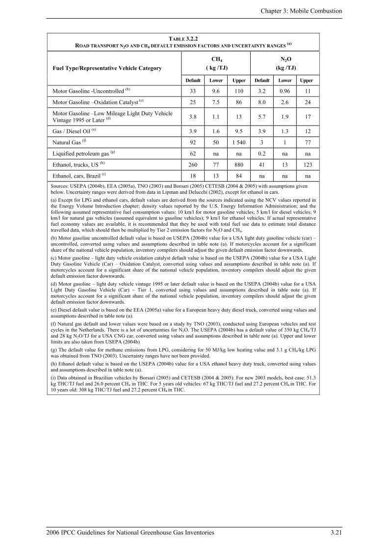
If CH4 and N2O emissions from mobile sources are not a key category, default CH4 and N2O emission factors presented in Table 3.2.2 may be used when national data are unavailable. When using these default values, inventory compilers should note the assumed fuel economy values that were used for unit conversions and the representative vehicle categories that were used as the basis of the default factors (see table notes for specific assumptions).
It is good practice to ensure that default emission factors, if selected, best represent local fuel quality/composition and combustion or emission control technology. If biofuels are included in national road transportation fuel use estimates, biofuel-specific emission factors should be used and associated CH4 and N2O emissions should be included in national totals.
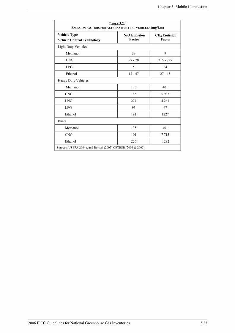
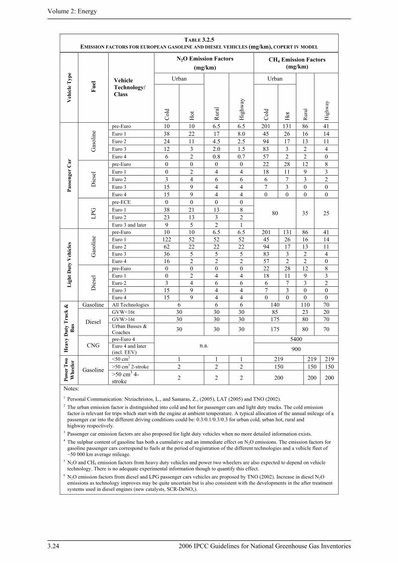
Because CH4 and N2O emission rates are largely dependent upon the combustion and emission control technology present, technology-specific emission factors should be used, if CH4 and N2O emissions from mobile sources are a key category. Tables 3.2.3 and 3.2.5 give potentially applicable Tier 2 and Tier 3 emission factors from US and European data respectively. In addition, the U.S. has developed emission factors for some alternative fuel vehicles (Table 3.2.4). The IPCC EFDB and scientific literature may also provide emission factors (or standard emission estimation models) which inventory compilers may use, if appropriate to national circumstances.
5 For example, biodiesel made from coal methanol with animal feedstocks has a non-zero fossil fuel fraction and is therefore
not fully carbon neutral. Ethanol from the fermentation of agricultural products will generally be purely biogenic (carbon neutral), except in some cases, such as fossil-fuel derived methanol. Products which have undergone further chemical transformation may contain substantial amounts of fossil carbon ranging from about 5-10 percent in the fossil methanol used for biodiesel production upwards to 46 percent in ethyl-tertiary-butyl-ether (ETBE) from fossil isobutene (ADEME/DIREM, 2002). Some processes may generate biogenic by-products such as glycol or glycerine, which may then be used elsewhere.

Volume 2: Energy
3.18 2006 IPCC Guidelines for National Greenhouse Gas Inventories
BOX 3.2.1 EXAMPLES OF BIOFUEL USE IN ROAD TRANSPORTATION
Examples of biofuel use in road transportation include:
• Ethanol is typically produced through the fermentation of sugar cane, sugar beets, grain, corn or potatoes. It may be used neat (100 percent, Brazil) or blended with gasoline in varying volumes (5-12 percent in Europe and North America, 10 percent in India, while 25 percent is common in Brazil). The biogenic portion of pure ethanol is 100 percent.
• Biodiesel is a fuel made from the trans-esterification of vegetable oils (e.g., rape, soy, mustard, sun-flower), animal fats or recycled cooking oils. It is non-toxic, biodegradable and essentially sulphur-free and can be used in any diesel engine either in its pure form (B100 or neat Biodiesel) or in a blend with petroleum diesel (B2 and B20, which contain 2 and 20 per cent biodiesel by volume). B100 may contain 10 percent fossil carbon from the methanol (made from natural gas) used in the esterification process.
• Ethyl-tertiary-butyl-ether (ETBE) is used as a high octane blending component in gasoline (e.g., in France and Spain in blends of up to 15 percent content). The most common source is the etherification of ethanol from the fermentation of sugar beets, grain and potatoes with fossil isobutene.
• Gaseous Biomass (landfill gas, sludge gas, and other biogas) produced by the anaerobic digestion of organic matter is occasionally used in some European countries (e.g. Sweden and Switzerland). Landfill and sewage gas are common sources of gaseous biomass currently.
Other potential future commercial biofuels for use in mobile combustion include those derived from lignocellulosic biomass. Lignocellulosic feedstock materials include cereal straw, woody biomass, corn stover (dried leaves and stems), or similar energy crops. A range of varying extraction and transformation processes permit the production of additional biogenic fuels (e.g., methanol,dimethyl-ether (DME), and methyl-tetrahydrofuran (MTHF)).
It is good practice to select or develop an emission factor based on all the following criteria: • Fuel type (gasoline, diesel, natural gas) considering, if possible, fuel composition (studies have shown that
decreasing fuel sulphur level may lead to significant reductions in N2O emissions6)
• Vehicle type (i.e. passenger cars, light trucks, heavy trucks, motorcycles)
• Emission control technology considering the presence and performance (e.g., as function of age) of catalytic converters (e.g., typical catalysts convert nitrogen oxides to N2, and CH4 into CO2). Díaz et al (2001) reports catalyst conversion efficiency for total hydrocarbons (THCs), of which CH4 is a component, of 92 (+/- 6) percent in a 1993-1995 fleet. Considerable deterioration of catalysts with relatively high mileage accumulation; specifically, THC levels remained steady until approximately 60 000 kilometers, then increased by 33 percent to between 60 000 to 100 000 kilometres.
• The impact of operating conditions (e.g., speed, road conditions, and driving patterns, which all affect fuel economy and vehicle systems’ performance)7.
• Consideration that any alternative fuel emission factor estimates tend to have a high degree of uncertainty, given the wide range of engine technologies and the small sample sizes associated with existing studies8.
The following section provides a method for developing CH4 emission factors from THC values. Well conducted and documented inspection and maintenance (I/M) programmes may provide a source of national data for emission factors by fuel, model, and year as well as annual mileage accumulation rates. Although some I/M programmes may only have available emission factors for new vehicles and local air pollutants, (sometimes called regulated pollutants, e.g. NOx, PM, NMVOCs, THCs), it may be possible to derive CH4 or N2O emission factors from these data. A CH4 emission factor may be calculated as the difference between emission factors for THCs and NMVOCs. In many countries, CH4 emissions from vehicles are not directly measured. They are a 6 UNFCCC (2004) 7 Lipman and Delucchi (2002) provide data and explanation of the impact of operating conditions on CH4 and N2O
emissions. 8 Some useful references on bio fuels are available in Beer et al (2000), CONCAWE (2002).

Chapter 3: Mobile Combustion
2006 IPCC Guidelines for National Greenhouse Gas Inventories 3.19
fraction of THCs, which is more commonly obtained through laboratory measurements. USEPA (1997) and Borsari (2005) and CETESB (2004 & 2005) provide conversion factors for reporting hydrocarbon emissions in different forms. Based on these sources, the following ratios of CH4 to THC may be used to develop CH4 emission factors from country-specific THC data9:
• 2-stroke gasoline: 0.9 percent,
• 4-stroke gasoline: 10-25 percent,
• diesel: 1.6 percent,
• LPG: 29.6 percent,
• natural gas vehicles: 88.0-95.2 percent,
• gasohol E22: 24.3-25.5 percent, and
• ethanol hydrated E100: 26.0-27.2 percent.
Some I/M programmes may collect data on evaporatives, which may be assumed to be equal to NMVOCs.10 Recent and ongoing research has investigated the relationship between N2O and NOx emissions. Useful data may become available from this work11.
Further refinements in the factors can be made if additional local data (e.g. on average driving speeds, climate, altitude, pollution control devices, or road conditions) are available, for example, by scaling emission factors to reflect the national circumstances by multiplying by an adjustment factor (e.g., traffic congestion or severe loading). Emission factors for both CH4 and N2O are established not just during a representative compliance driving test, but also specifically tested during running conditions and cold start conditions. Thus, data collected on the driving patterns in a country (based on the relationship of starts to running distances) can be used to adjust the emission factors for CH4 and N2O. Although ambient temperature has been shown to have impacts on local air pollutants, there is limited research on the effects of temperature on CH4 and N2O (USEPA 2004b). Please see Box 3.2.2 for information on refining emission factors for mobile sources in developing countries.
9 Gamas et. al. (1999) and Díaz, et.al (2001) report measured THC data for a range of vehicle vintage and fuel types.
10 IPCC (1997). 11 For light motor vehicles and passenger cars, ratios N2O/NOx obtained in literature range around 0.10-0.25 (Lipmann and
Delucchi, 2002 and Behrentz, 2003).

Volume 2: Energy
3.20 2006 IPCC Guidelines for National Greenhouse Gas Inventories
BOX 3.2.2 REFINING EMISSION FACTORS FOR MOBILE SOURCES IN DEVELOPING COUNTRIES
In some developing countries, the estimated emission rates per kilometre travelled may need to be altered to accommodate national circumstances, which could include:
•Technology variations - In many cases due to tampering of emission control systems, fuel adulteration, or simply vehicle age, some vehicles may be operating without a functioning catalytic converter. Consequently, N2O emissions may be low and CH4 may be high when catalytic converters are not present or operating improperly. Díaz et al (2001) provides information on THC values for Mexico City and catalytic converter efficiency as a function of age and mileage, and this also chapter provides guidance on developing CH4 factors from THC data.
▪ Engine loading - Due to traffic density or challenging topography, the number of accelerations and decelerations that a local vehicle encounters may be significantly greater than that for corresponding travel in countries where emission factors were developed. This happens when these countries have well established road and traffic control networks. Increased engine loading may correlate with higher CH4 and N2O emissions.
▪ Fuel Composition - Poor fuel quality and high or varying sulphur content may adversely affect the performance of engines and conversion efficiency of post-combustion emission control devices such as catalytic converters. For example, N2O emission rates have been shown to increase with the sulphur content in fuels (UNFCCC, 2004). The effects of sulphur content on CH4 emissions are not known. Refinery data may indicate production quantities on a national scale.
Section 3.2.2 Uncertainty Assessment provides information on how to develop uncertainty estimates for emission factors for road transportation.
Further information on emission factors for developing countries is available from Mitra et al. (2004).
Chapter 3: Mobile Combustion
2006 IPCC Guidelines for National Greenhouse Gas Inventories 3.21
TABLE 3.2.2 ROAD TRANSPORT N2O AND CH4 DEFAULT EMISSION FACTORS AND UNCERTAINTY RANGES (a)
CH4 ( kg /TJ)
N2O (kg /TJ) Fuel Type/Representative Vehicle Category
Default Lower Upper Default Lower Upper
Motor Gasoline -Uncontrolled (b) 33 9.6 110 3.2 0.96 11
Motor Gasoline –Oxidation Catalyst (c) 25 7.5 86 8.0 2.6 24
Motor Gasoline –Low Mileage Light Duty Vehicle Vintage 1995 or Later (d) 3.8 1.1 13 5.7 1.9 17
Gas / Diesel Oil (e) 3.9 1.6 9.5 3.9 1.3 12
Natural Gas (f) 92 50 1 540 3 1 77
Liquified petroleum gas (g) 62 na na 0.2 na na
Ethanol, trucks, US (h) 260 77 880 41 13 123
Ethanol, cars, Brazil (i) 18 13 84 na na na
Sources: USEPA (2004b), EEA (2005a), TNO (2003) and Borsari (2005) CETESB (2004 & 2005) with assumptions given below. Uncertainty ranges were derived from data in Lipman and Delucchi (2002), except for ethanol in cars. (a) Except for LPG and ethanol cars, default values are derived from the sources indicated using the NCV values reported in the Energy Volume Introduction chapter; density values reported by the U.S. Energy Information Administration; and the following assumed representative fuel consumption values: 10 km/l for motor gasoline vehicles; 5 km/l for diesel vehicles; 9 km/l for natural gas vehicles (assumed equivalent to gasoline vehicles); 9 km/l for ethanol vehicles. If actual representative fuel economy values are available, it is recommended that they be used with total fuel use data to estimate total distance travelled data, which should then be multiplied by Tier 2 emission factors for N2O and CH4. (b) Motor gasoline uncontrolled default value is based on USEPA (2004b) value for a USA light duty gasoline vehicle (car) – uncontrolled, converted using values and assumptions described in table note (a). If motorcycles account for a significant share of the national vehicle population, inventory compilers should adjust the given default emission factor downwards. (c) Motor gasoline – light duty vehicle oxidation catalyst default value is based on the USEPA (2004b) value for a USA Light Duty Gasoline Vehicle (Car) – Oxidation Catalyst, converted using values and assumptions described in table note (a). If motorcycles account for a significant share of the national vehicle population, inventory compilers should adjust the given default emission factor downwards. (d) Motor gasoline – light duty vehicle vintage 1995 or later default value is based on the USEPA (2004b) value for a USA Light Duty Gasoline Vehicle (Car) – Tier 1, converted using values and assumptions described in table note (a). If motorcycles account for a significant share of the national vehicle population, inventory compilers should adjust the given default emission factor downwards. (e) Diesel default value is based on the EEA (2005a) value for a European heavy duty diesel truck, converted using values and assumptions described in table note (a). (f) Natural gas default and lower values were based on a study by TNO (2003), conducted using European vehicles and test cycles in the Netherlands. There is a lot of uncertainties for N2O. The USEPA (2004b) has a default value of 350 kg CH4/TJ and 28 kg N2O/TJ for a USA CNG car, converted using values and assumptions described in table note (a). Upper and lower limits are also taken from USEPA (2004b) (g) The default value for methane emissions from LPG, considering for 50 MJ/kg low heating value and 3.1 g CH4/kg LPG was obtained from TNO (2003). Uncertainty ranges have not been provided. (h) Ethanol default value is based on the USEPA (2004b) value for a USA ethanol heavy duty truck, converted using values and assumptions described in table note (a). (i) Data obtained in Brazilian vehicles by Borsari (2005) and CETESB (2004 & 2005). For new 2003 models, best case: 51.3 kg THC/TJ fuel and 26.0 percent CH4 in THC. For 5 years old vehicles: 67 kg THC/TJ fuel and 27.2 percent CH4 in THC. For 10 years old: 308 kg THC/TJ fuel and 27.2 percent CH4 in THC.

Volume 2: Energy
3.22 2006 IPCC Guidelines for National Greenhouse Gas Inventories
TABLE 3.2.3 N2O AND CH4 EMISSION FACTORS FOR USA GASOLINE AND DIESEL VEHICLES
N2O CH4
Running (hot)
Cold Start
Running (hot)
Cold Start
Vehicle Type Emission Control Technology
mg/km mg/start mg/km mg/start
Low Emission Vehicle (LEV) 0 90 6 32
Advanced Three-Way Catalyst 9 113 7 55
Early Three-Way Catalyst 26 92 39 34
Oxidation Catalyst 20 72 82 9
Non-oxidation Catalyst 8 28 96 59
Light Duty Gasoline Vehicle (Car)
Uncontrolled 8 28 101 62
Advanced 1 0 1 -3
Moderate 1 0 1 -3 Light Duty Diesel Vehicle (Car)
Uncontrolled 1 -1 1 -3
Low Emission Vehicle (LEV) 1 59 7 46
Advanced Three-Way Catalyst 25 200 14 82
Early Three-Way Catalyst 43 153 39 72
Oxidation Catalyst 26 93 81 99
Non-oxidation catalyst 9 32 109 67
Light Duty Gasoline Truck
Uncontrolled 9 32 116 71
Advanced and moderate 1 -1 1 -4 Light Duty Diesel Truck Uncontrolled 1 -1 1 -4
Low Emission Vehicle (LEV) 1 120 14 94
Advanced Three-Way Catalyst 52 409 15 163
Early Three-Way Catalyst 88 313 121 183
Oxidation catalyst 55 194 111 215
Non-oxidation catalyst 20 70 239 147
Heavy Duty Gasoline Vehicle
Heavy Duty Gasoline Vehicle - Uncontrolled 21 74 263 162
Heavy Duty Diesel Vehicle
All -advanced, moderate, or uncontrolled 3 -2 4 -11
Non-oxidation catalyst 3 12 40 24 Motorcycles
Uncontrolled 4 15 53 33
Source: USEPA (2004b). Notes: a These data have been rounded to whole numbers. b Negative emission factors indicate that a vehicle starting cold produces fewer emissions than a vehicle starting warm or running warming. c A database of technology dependent emission factors based on European data is available in the COPERT tool at http://vergina.eng.auth.gr/mech0/lat/copert/copert.htm. d Because of the total-hydrocarbon limits in Europe, the CH4-emissions of European vehicles may be lower than the indicated values from USA (Heeb, et. al., 2003) e These “cold starts” were measured at an ambient temperature of 68ºF to 86ºF (20°C to 30°C).
Chapter 3: Mobile Combustion
2006 IPCC Guidelines for National Greenhouse Gas Inventories 3.23
TABLE 3.2.4 EMISSION FACTORS FOR ALTERNATIVE FUEL VEHICLES (mg/km)
Vehicle Type Vehicle Control Technology
N2O Emission Factor
CH4 Emission Factor
Light Duty Vehicles
Methanol 39 9
CNG 27 - 70 215 - 725
LPG 5 24
Ethanol 12 - 47 27 - 45
Heavy Duty Vehicles
Methanol 135 401
CNG 185 5 983
LNG 274 4 261
LPG 93 67
Ethanol 191 1227
Buses
Methanol 135 401
CNG 101 7 715
Ethanol 226 1 292
Sources: USEPA 2004c, and Borsari (2005) CETESB (2004 & 2005).
Volume 2: Energy
3.24 2006 IPCC Guidelines for National Greenhouse Gas Inventories
TABLE 3.2.5 EMISSION FACTORS FOR EUROPEAN GASOLINE AND DIESEL VEHICLES (mg/km), COPERT IV MODEL
N2O Emission Factors (mg/km)
CH4 Emission Factors (mg/km)
Urban Urban
Veh
icle
Typ
e
Fuel
Vehicle Technology/ Class
Col
d
Hot
Rur
al
Hig
hway
Col
d
Hot
Rur
al
Hig
hway
pre-Euro 10 10 6.5 6.5 201 131 86 41 Euro 1 38 22 17 8.0 45 26 16 14 Euro 2 24 11 4.5 2.5 94 17 13 11 Euro 3 12 3 2.0 1.5 83 3 2 4 G
asol
ine
Euro 4 6 2 0.8 0.7 57 2 2 0 pre-Euro 0 0 0 0 22 28 12 8 Euro 1 0 2 4 4 18 11 9 3 Euro 2 3 4 6 6 6 7 3 2 Euro 3 15 9 4 4 7 3 0 0 D
iese
l
Euro 4 15 9 4 4 0 0 0 0 pre-ECE 0 0 0 0 Euro 1 38 21 13 8 Euro 2 23 13 3 2
Pass
enge
r C
ar
LPG
Euro 3 and later 9 5 2 1
80 35 25
pre-Euro 10 10 6.5 6.5 201 131 86 41 Euro 1 122 52 52 52 45 26 16 14 Euro 2 62 22 22 22 94 17 13 11 Euro 3 36 5 5 5 83 3 2 4 G
asol
ine
Euro 4 16 2 2 2 57 2 2 0 pre-Euro 0 0 0 0 22 28 12 8 Euro 1 0 2 4 4 18 11 9 3 Euro 2 3 4 6 6 6 7 3 2 Euro 3 15 9 4 4 7 3 0 0
Lig
ht D
uty
Veh
icle
s
Die
sel
Euro 4 15 9 4 4 0 0 0 0 Gasoline All Technologies 6 6 6 140 110 70
GVW<16t 30 30 30 85 23 20 GVW>16t 30 30 30 175 80 70 Diesel Urban Busses & Coaches 30 30 30 175 80 70 pre-Euro 4 5400
Hea
vy D
uty
Tru
ck &
B
us
CNG Euro 4 and later (incl. EEV)
n.a. 900 <50 cm3 1 1 1 219 219 219 >50 cm3 2-stroke 2 2 2 150 150 150
Pow
er T
wo
Whe
eler
Gasoline >50 cm3 4-stroke 2 2 2 200 200 200
Notes: 1 Personal Communication: Ntziachristos, L., and Samaras, Z., (2005), LAT (2005) and TNO (2002). 2 The urban emission factor is distinguished into cold and hot for passenger cars and light duty trucks. The cold emission factor is relevant for trips which start with the engine at ambient temperature. A typical allocation of the annual mileage of a passenger car into the different driving conditions could be: 0.3/0.1/0.3/0.3 for urban cold, urban hot, rural and highway respectively. 3 Passenger car emission factors are also proposed for light duty vehicles when no more detailed information exists. 4 The sulphur content of gasoline has both a cumulative and an immediate effect on N2O emissions. The emission factors for gasoline passenger cars correspond to fuels at the period of registration of the different technologies and a vehicle fleet of ~50 000 km average mileage. 5 N2O and CH4 emission factors from heavy duty vehicles and power two wheelers are also expected to depend on vehicle technology. There is no adequate experimental information though to quantify this effect. 6 N2O emission factors from diesel and LPG passenger cars vehicles are proposed by TNO (2002). Increase in diesel N2O emissions as technology improves may be quite uncertain but is also consistent with the developments in the after treatment systems used in diesel engines (new catalysts, SCR-DeNOx).
Chapter 3: Mobile Combustion
2006 IPCC Guidelines for National Greenhouse Gas Inventories 3.25
3.2.1.3 CHOICE OF ACTIVITY DATA Activity data may be provided either by fuel consumption or by vehicle kilometres travelled VKT. Use of adequate VKT data can be used to check top-down inventories.
FUEL CONSUMPTION
Emissions from road vehicles should be attributed to the country where the fuel is sold; therefore fuel consumption data should reflect fuel that is sold within the country’s territories. Such energy data are typically available from the national statistical agency. In addition to fuel sold data collected nationally, inventory compilers should collect activity data on other fuels used in that country with minor distributions that are not part of the national statistics (i.e., fuels that are not widely consumed, including those in niche markets such as compressed natural gas or biofuels). These data are often also available from the national statistical agency or they may be accounted for under separate tax collection processes. For Tier 3 methods, the MOBILE or COPERT models may help develop activity data.
It is good practice to check the following factors (as a minimum) before using the fuel sold data:
• Does the fuel data relate to on-road only or include off-road vehicles as well? National statistics may report total transportation fuel without specifying fuel consumed by on-road and off-road activities. It is important to ensure that fuel use data for road vehicles excludes that used for off-road vehicles or machinery (see Off-Road Transportation Section 3.3). Fuels may be taxed differently based on their intended use. A Road-Taxed fuel survey may provide an indication of the quantity of fuel sold for on-road use. Typically, the on-road vehicle fleet and associated fuel sales are better documented than the off-road vehicle population and activity. This fact should be considered when developing emission estimates.
• Is agricultural fuel use included? Some of this may be stationary use while some will be for mobile sources. However, much of this will not be on-road use and should not be included here.
• Is fuel sold for transportation uses used for other purposes (e.g., as fuel for a stationary boiler), or vice versa? For example, in countries where kerosene is subsidized to lower its price for residential heating and cooking, the national statistics may allocate the associated kerosene consumption to the residential sector even though substantial amounts of kerosene may have been blended into and consumed with transportation fuels.
• How are biofuels accounted for?
• How are blended fuels reported and accounted for? Accounting for official blends (e.g. addition of 25 percent of ethanol in gasoline) in activity data is straightforward, but if fuel adulteration or tampering (e.g. spent solvents in gasoline, kerosene in diesel fuel) is prevalent in a country, appropriate adjustments should be applied to fuel data, taking care to avoid double counting.
• Are the statistics affected by fuel tourism?
• Is there significant fuel smuggling?
• How is the use of lubricants as an additive in 2-stroke fuels reported? It may be included in the road transport fuel use or may be reported separately as a lubricant (see Box 3.2.4.).
Two alternative approaches are suggested to separate non-road and on-road fuel use:
(1) For each major fuel type, estimate the fuel used by each road vehicle type from vehicle kilometres travelled data. The difference between this road vehicle total and the apparent consumption is attributed to the off-road sector; or
(2) The same fuel-specific estimate in (1) is supplemented by a similarly structured bottom-up estimate of off-road fuel use from a knowledge of the off-road equipment types and their usage. The apparent consumption in the transportation sector is then disaggregated according to each vehicle type and the off-road sector in proportion to the bottom-up estimates.
Depending on national circumstances, inventory compilers may need to adjust national statistics on road transportation fuel use to prevent under- or over-reporting emissions from road vehicles. It is good practice to adjust national fuel sales statistics to ensure that the data used just reflects on-road use. Where this adjustment is necessary it is good practice to cross-check with the other appropriate sectors to ensure that any fuel removed from on-road statistics is added to the appropriate sector, or vice versa.
As validation, and if distance travelled data are available (see below vehicle kilometres travelled), it is good practice to estimate fuel use from the distance travelled data. The first step (Equation 3.2.6) is to estimate fuel consumed by vehicle type i and fuel type j.

Volume 2: Energy
3.26 2006 IPCC Guidelines for National Greenhouse Gas Inventories
EQUATION 3.2.6 VALIDATING FUEL CONSUMPTION ∑ ••=
tji tjinConsumptiotjitanceDistjiVehiclesFuelEstimated,,
],,,,,,[
Where:
Estimated Fuel =total estimated fuel use estimated from distance travelled (VKT) data (l)
Vehiclesi,j,t = number of vehicles of type i and using fuel j on road type t
Distancei,j,t = annual kilometres travelled per vehicle of type i and using fuel j on road type t (km)
Consumptioni,j,t = average fuel consumption (l/km) by vehicles of type i and using fuel j on road type t
i = vehicle type (e.g., car, bus)
j = fuel type (e.g. motor gasoline, diesel, natural gas, LPG)
t = type of road (e.g., urban, rural)
If data are not available on the distance travelled on different road types, this equation should be simplified by removing the “t” the type of road. More detailed estimates are also possible including the additional fuel used during the cold start phase.
It is good practice to compare the fuel sold statistics used in the Tier 1 approach with the result of equation 3.2.6. It is good practice to consider any differences and determine which data is of higher quality. Except in rare cases (e.g. large quantities of fuel sold for off-road uses, extensive fuel smuggling), fuel sold statistics are likely to be more reliable. This provides an important quality check. Significant differences between the results of two approaches may indicate that one or both sets of statistics may have errors, and that there is need for further analysis. Areas of investigation to pursue when reconciling fuel sold statistics and vehicle kilometre travelled data are listed in Section 3 2.3, Inventory quality assurance/quality control (QA/QC).
Distance travelled data for vehicles by type and fuel are important underpinnings for the higher tier calculations of CH4 and N2O emissions from road transport. So it may be necessary to adjust the distance travelled data to be consistent with the fuel sold data before proceeding to estimating emissions of CH4 and N2O. This is especially important in cases where the discrepancy between the estimated fuel use (Eq 3.2.6) and the statistical fuel sold is significant compared to the uncertainties in fuel sold statistics. Inventory compilers will have to use their judgement on the best way of adjusting distance travelled data. This could be done pro rata with the same adjustment factor applied to all vehicle type and road type classes or, where some data are judged to be more accurate, different adjustments could be applied to different vehicle types and road types. An example of the latter could be where the data on vehicle travelled on major highways is believed to be reasonably well known and on the other hand rural traffic is poorly measured. In any case, the adjustments made for reasons of the choice of adjustment factor and background data as well as any other checks should be well documented and reviewed.
VEHICLE KILOMETRES TRAVELLED (VKT)
While fuel data can be used at Tier 1 for CH4 and N2O, higher tiers also need vehicle kilometres travelled (VKT) by vehicle type, fuel type and possibly road type as well.
Many countries collect, measure, or otherwise estimate VKT. Often this is done by sample surveys counting vehicle numbers passing fixed points. These surveys can be automatic or manual and count vehicle numbers by type of vehicle. There may be differences between the vehicle classification used in the counts and other data (e.g. tax classes) that also give data on vehicle numbers. In addition they are unlikely to differentiate between similar vehicle using different fuels (e.g. motor gasoline and diesel cars). Sometimes more detailed information is also collected (e.g. vehicle speeds as well as numbers) especially where more detailed traffic planning has been performed. This may only be available for a municipality rather than the whole country. From these traffic counts, transport authorities can make estimates of the total VKT travelled in a country. Alternatives ways to determine the mileage are direct surveys of vehicle owners (private and commercial) and use of administrative records for commercial vehicles, taking care to account for outdated registration records for scrapped vehicles (Box 3.2.3 provides an approach to estimate the remaining fleets).
Where VKT is estimated in a country it is good practice to use this data, especially to validate the fuel sold data (see section 3.2.1.4).

Chapter 3: Mobile Combustion
2006 IPCC Guidelines for National Greenhouse Gas Inventories 3.27
OTHER PARAMETERS.
If CH4 or N2O emissions from road transportation are a key category, it is good practice to obtain more information on parameters that influence emission factors to ensure the activity data is compatible with the applicable Tier 2 or Tier 3 emission factor. This will require more dissagregated activity data in order to implement Equation 3.2.3 or 3.2.5:
• the amount of fuel consumed (in terajoules) by fuel type (all tiers);
• for each fuel type, the amount of fuel (or VKT driven) that is consumed by each representative vehicle type (e.g., passenger, light-duty or heavy-duty for road vehicles) preferably with age categories (Tiers 2 and 3); and
• the emission control technology (e.g., three-way catalysts) (Tiers 2 and 3).
• It may also be possible to collect VKT data by type of road (e.g. urban, rural, highway)
If the distribution of fuel use by vehicle and fuel type is unknown, it may be estimated from the number of vehicles by type. If the number of vehicles by vehicle and fuel type is not known, it may be estimated from national statistics (see below).
Vehicle technology, which is usually directly linked to the model and year of vehicle, affects CH4 and N2O emissions. Therefore, for Tier 2 and Tier 3 methods, activity data should be grouped based on Original Equipment Manufacturer (OEM) emission control technologies fitted to vehicle types in the fleet. The fleet age distribution helps stratify the fleet into age and subsequently technology classes. If the distribution is not available, vehicle deterioration curves may be used to estimate vehicle lifespan and therefore the number of vehicles remaining in service based on the number introduced annually (see Box 3.2.3).
In addition, if possible, determine (through estimates or from national statistics) the total distance travelled (i.e., VKT) by each vehicle technology type (Tier 3). If VKT data are not available, they can be estimated based on fuel consumption and assumed national fuel economy values. To estimate VKT using road transport fuel use data, convert fuel data to volume units (litres) and then multiply the fuel-type total by an assumed fuel economy value representative of the national vehicle population for that fuel type (km/l).
If using the Tier 3 method and national VKT statistics are available, the fuel consumption associated with these distance-travelled figures should be calculated and aggregated by fuel for comparison with national energy balance figures. Like the Tier 2 method, for Tier 3 it is suggested to further subdivide each vehicle type into uncontrolled and key classes of emission control technology. It should be taken into consideration that typically, emissions and distance travelled each year vary according to the age of the vehicle; the older vehicles tend to travel less but may emit more CH4 and N2O per unit of activity. Some vehicles, especially in developing countries, may have been converted to operate on a different type of fuel than their original design.
To implement the Tier 2 or 3 method, activity data may be derived from a number of possible sources. Vehicle inspection and maintenance (I/M) programmes, where operating, may provide insight into annual mileage accumulation rates. National vehicle licensing records may provide fleet information (counts of vehicles per model-year per region) and may even record mileage between license renewals. Other sources for developing activity data include vehicle sales, import, and export records.
Alternatively, vehicle stocks may be estimated from the number of new vehicle imports and sales by type, fuel and model year. The populations of vehicles remaining in service may be estimated by applying scrappage or attrition curves.
Higher tier methods involving an estimate of cold start emissions require knowledge of the number of starts. This can be derived from the total distance travelled and the average trip length. Typically, this can be obtained from traffic surveys. This data is often collected for local or traffic studies for transport planning.
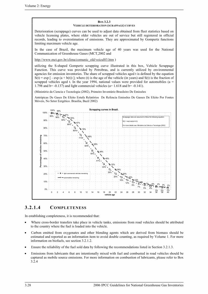
Volume 2: Energy
3.28 2006 IPCC Guidelines for National Greenhouse Gas Inventories
BOX 3.2.3 VEHICLE DETERIORATION (SCRAPPAGE) CURVES
Deterioration (scrappage) curves can be used to adjust data obtained from fleet statistics based on vehicle licensing plates, where older vehicles are out of service but still registered in official records, leading to overestimation of emissions. They are approximated by Gompertz functions limiting maximum vehicle age.
In the case of Brazil, the maximum vehicle age of 40 years was used for the National Communication of Greenhouse Gases (MCT,2002 and
http://www.mct.gov.br/clima/comunic_old/veicul03.htm )
utilizing the S-shaped Gompertz scrapping curve illustrated in this box, Vehicle Scrappage Function. This curve was provided by Petrobras, and is currently utilized by environmental agencies for emission inventories. The share of scrapped vehicles aged t is defined by the equation S(t) = exp [ - exp (a + b(t)) ]; where (t) is the age of the vehicle (in years) and S(t) is the fraction of scrapped vehicles aged t. In the year 1994, national values were provided for automobiles (a = 1.798 and b= -0.137) and light commercial vehicles (a= 1.618 and b= -0.141).
(Ministério da Ciencia e Tecnologia (2002), Primeiro Inventário Brasileiro De Emissões
Antrópicas De Gases De Efeito Estufa Relatórios De Refencia Emissões De Gasses De Efeito Por Fontes Móveis, No Setor Eergético. Brasília, Bazil 2002)
Scrapping curves in Brazil.
99% 98%94%
89%
80%
71%
60%
50%
41%
33%
26%
20%
16%12%
9%7% 5%
2%
97%93%
87%
78%
59%
49%
40%
32%
26%
20%16%
12%9%
7%
2%4%
3%
2%3%4%6%
99%100%
69%
0%
10%
20%
30%
40%
50%
60%
70%
80%
90%
100%
0 2 4 6 8 10 12 14 16 18 20 22 24 26 28 30 32 34 36 38 40vehicle age
Perc
enta
ge o
f veh
icle
s re
mai
ning
light commercial vehicles remaining
automobiles remaining
Scrappage rates are assumed to follow the following equation:
S(t) = exp(-exp(a+b·t))
For more details see: Ministério da Ciência e Tecnologia (2002)
3.2.1.4 COMPLETENESS In establishing completeness, it is recommended that:
• Where cross-border transfers take place in vehicle tanks, emissions from road vehicles should be attributed to the country where the fuel is loaded into the vehicle.
• Carbon emitted from oxygenates and other blending agents which are derived from biomass should be estimated and reported as an information item to avoid double counting, as required by Volume 1. For more information on biofuels, see section 3.2.1.2.
• Ensure the reliability of the fuel sold data by following the recommendations listed in Section 3.2.1.3.
• Emissions from lubricants that are intentionally mixed with fuel and combusted in road vehicles should be captured as mobile source emissions. For more information on combustion of lubricants, please refer to Box 3.2.4

Chapter 3: Mobile Combustion
2006 IPCC Guidelines for National Greenhouse Gas Inventories 3.29
BOX 3.2.4 LUBRICANTS IN MOBILE COMBUSTION
Lubrication of a two-stroke petrol engine is conceptually quite different from that of a four-stroke engine, as it is not possible to have a separate lubricating oil sump. A two-stroke petrol engine should be lubricated by a mixture of lubricating oil and petrol in suitable proportion according to the manufacturer's recommendations. Depending on the engine type, mixtures of 1:25, 1:33 and 1:50 are common.
In the latest generation two-stroke engines, the lubricating oil is directly injected by an accurate metering device from a separate tank into the petrol in quantities that depend on the speed and load of the engine. Older or inexpensive two-stroke engines will receive the lubricant as part of the fuel mixture. Often these mixtures are prepared by the fuel supplier and delivered to the gas station but sometimes the vehicle owner will add oil at the service station. In some countries two stroke engines have been historically very significant as recent as the 1990’s (e.g. Eastern Europe) or are still very significant (e.g. India and parts of South-East Asia).
The classification of these lubricants in energy statistics as lubricant or fuel may vary. Inventory compilers need to make sure that these lubricants are allocated to end use appropriately, accounted for properly, and that double counting or omission is avoided (compare treatment of lubricants in Volume 3 Chapter 5: Non-energy product and feedstock use of fuels). Lubricants intentionally mixed with fuel and combusted in road vehicles should be reported as energy and the associated emissions calculated using mobile source guidelines. When the chosen activity data for 2-stroke engines are based on kilometres travelled, the added lubricants should be considered in the fuel economy, as a part of the fuel blend.
3.2.1.5 DEVELOPING A CONSISTENT TIME SERIES When data collection and accounting procedures, emission estimation methodologies, or models are revised, it is good practice to recalculate the complete time series. A consistent time series with regard to initial collection of fleet technology data may require extrapolation, possibly supported by the use of proxy data. This is likely to be needed for early years. Inventory compilers should refer to the discussion in Volume 1 Chapter 5: Time Series Consistency for general guidance.
Since this chapter contains many updated emission factors, for CO2 (accounting for 100 percent fuel oxidation), CH4, and N2O, inventory compilers should ensure time series consistency. A consistent time series should consider the technological change in vehicles and their catalysts control systems. The time series should take into account the gradual phase-in among fleets, which is driven by legislation and market forces. Consistency can be maintained with accurate data on fleet distribution according to engine and control system technology, maintenance, control technology obsolescence, and fuel type. If VKT are not available for the whole time series but for a recent year, guidelines in Volume 1 Chapter 5: Time Series Consistency should be used to select a splicing method.
3.2.2 Uncertainty Assessment CO2, N2O, and CH4 contribute typically around 97, 2-3 and 1 percent of CO2-equivalent emissions from the road transportation sector, respectively. Therefore, although uncertainties in N2O and CH4 estimates are much higher, CO2 dominates the emissions from road transport. Use of locally estimated data will reduce uncertainties, particularly with bottom-up estimates.
Emission factor uncertainty For CO2, the uncertainty in the emission factor is typically less than 2 percent when national values are used (see Table 1.4 of the Introduction Chapter of this Volume). Default CO2 emission factors given in Table 3.2.1. Road Transport Default Carbon Dioxide Emission Factors have an uncertainty of 2-5 percent), due to uncertainty in the fuel composition. Use of fuel blends, e.g. involving biofuels, or adulterated fuels may increase the uncertainty in emission factors if the composition of the blend is uncertain.
The uncertainties in emission factors for CH4 and N2O are typically relatively high (especially for N2O) and are likely to be a factor of 2-3. They depend on:
• Uncertainties in fuel composition (including the possibility of fuel adulteration) and sulphur content;
Volume 2: Energy
3.30 2006 IPCC Guidelines for National Greenhouse Gas Inventories
• Uncertainties in fleet age distribution and other characterisation of the vehicle stock, including cross-border effects - the technical characteristics of vehicles from another country that take on fuel may be covered by technology models;
• Uncertainties in maintenance patterns of the vehicle stock;
• Uncertainties in combustion conditions (climate, altitude) and driving practices, such as speed, proportion of running distance to cold starts, or load factors (CH4 and N2O);
• Uncertainties in application rates of post-combustion emission control technologies (e.g. three-way catalyst);
• Uncertainties in the use of additives to minimize the aging effect of catalysts;
• Uncertainties in operating temperatures (N2O); and
• Uncertainties of test equipment and emission measurement equipment.
It is good practice to estimate uncertainty based on published studies from which the emission factors were obtained. At least the following types of uncertainties may be discussed in published sources and need to be considered in the development of national emission factors from empirical data:
• A range in the emission factor of an individual vehicle, represented as a variance of measurements, due to variable emissions in different operating conditions (e.g. speed, temperature); and
• Uncertainty in the mean of emission factors of vehicles within the same vehicle class.
In addition, the vehicle sample that was measured may have been quite limited, or even a more robust sample of measurements may not be representative of the national fleet. Test driving cycles cannot fully reflect real driving behaviour, so at least some emission factor studies now test cold start emissions separately from running emissions, so that countries may be able to create country-specific adjustments, though those adjustments will themselves require more data collection with its own uncertainties.
Another source of uncertainty may be the conversion of the emission factor into units in which the activity data are given (e.g. from kg/GJ to g/km) because this requires additional assumptions about other parameters, such as fuel economy, which have an associated uncertainty as well.
The uncertainty in the emission factor can be reduced by stratifying vehicle fleets further by technology, age and driving conditions.
Activity data uncertainty Activity data are the primary source of uncertainty in the emission estimate. Activity data are either given in energy units (e.g. TJ) or other units for different purposes such as person-/ton-kilometres, vehicle stocks, trip length distributions, fuel efficiencies, etc. Possible sources of uncertainty, which will typically be about +/-5 percent, include:
• Uncertainties in national energy surveys and data returns;
• Unrecorded cross-border transfers;
• Misclassification of fuels;
• Misclassification in vehicle stock;
• Lack of completeness (fuel not recorded in other source categories may be used for transportation purposes); and
• Uncertainty in the conversion factor from one set of activity data to another (e.g. from fuel consumption data to person-/ton-kilometres, or vice versa, see above).
Stratification of activity data may reduce uncertainty, if they can be connected to results from a top-down fuel use approach.
For estimating CH4 and N2O emissions, a different tier and hence different sets of activity data may be used. It is good practice to ensure that top-down and bottom-up approaches match, and to document and explain deviations if they do not match (see also Section 3.2.1.4 Completeness). For these gases, the emission factor uncertainty will dominate and the activity data uncertainty may be taken to be the same as for CO2.
Further guidance on uncertainty estimates for activity data can be found in Volume 1 Chapter 3: Uncertainties.
Chapter 3: Mobile Combustion
2006 IPCC Guidelines for National Greenhouse Gas Inventories 3.31
3.2.3 Inventory Quality Assurance/Quality Control (QA/QC)
It is good practice to conduct quality control checks as outlined in Volume 1 Chapter 6: Quality Assurance/Quality Control and Verification and expert review of the emission estimates. Additional quality control checks as outlined in Tier 2 procedures in the same chapter and quality assurance procedures may also be applicable, particularly if higher tier methods are used to determine emissions from this source category. Inventory compilers are encouraged to use higher tier QA/QC for source categories as identified in Volume 1 Chapter 4: Methodological Choice and Identification of Key Categories.
In addition to the guidance in the referenced chapters, specific procedures of relevance to this source category are outlined below.
Comparison of emissions using alternative approaches
For CO2 emissions, the inventory compiler should compare estimates using both the fuel statistics and vehicle kilometre travelled data. Any anomalies between the emission estimates should be investigated and explained. The results of such comparisons should be recorded for internal documentation. Revising the following assumptions could narrow a detected gap between the approaches:
Off-road/non transportation fuel uses;
Annual average vehicle mileage;
Vehicle fuel efficiency;
Vehicle breakdowns by type, technology, age, etc.;
Use of oxygenates/biofuels/other additives;
Fuel use statistics; and
Fuel sold/used.
Review of emission factors
If default emission factors are used, the inventory compiler should ensure that they are applicable and relevant to the categories. If possible, the default factors should be compared to local data to provide further indication that the factors are applicable.
For CH4 and N2O emissions, the inventory compiler should ensure that the original data source for the local factors is applicable to the category and that accuracy checks on data acquisition and calculations have been performed. Where possible, the default factors and the local factors should be compared. If the default factors were used to estimate N2O emissions, the inventory compiler should ensure that the revised emission factors in Table 3.2.3 were used in the calculation.
Activity data check
The inventory compiler should review the source of the activity data to ensure applicability and relevance to the category. Section 3.2.1.3 provides good practice for checking activity data. Where possible, the inventory compiler should compare the data to historical activity data or model outputs to detect possible anomalies. The inventory compiler should ensure the reliability of activity data regarding fuels with minor distribution; fuel used for other purposes, on- and off-road traffic, and illegal transport of fuel in or out of the country. The inventory compiler should also avoid double counting of agricultural and off-road vehicles.
External review
The inventory compiler should perform an independent, objective review of the calculations, assumptions, and documentation of the emissions inventory to assess the effectiveness of the QC programme. The peer review should be performed by expert(s) who are familiar with the source category and who understand the inventory requirements. The development of CH4 and N2O emission factors is particularly important due to the large uncertainties in the default factors.

Volume 2: Energy
3.32 2006 IPCC Guidelines for National Greenhouse Gas Inventories
3.2.4 Reporting and Documentation It is good practice to document and archive all information required to produce the national emissions inventory estimates.
It is not practical to include all documentation in the national inventory report. However, the inventory should include summaries of methods used and references to source data such that the reported emissions estimates are transparent and steps in their calculation may be retraced. This applies particularly to national models used to estimate emissions from road transport, and to work done to improve knowledge of technology-specific emission factors for nitrous oxide and methane, where the uncertainties are particularly great. This type of information, provided the documentation is clear, should be submitted for inclusion in the EFDB.
Confidentiality is not likely to be a major issue with regard to road emissions, although it is noted that in some countries the military use of fuel may be kept confidential. The composition of some additives is confidential, but this is only important if it influences greenhouse gas emissions.
Where a model such as the USEPA MOVES or MOBILE models or the EEA COPERT model is used (EPA 2005a, EPA 2005b, EEA 2005, respectively), a complete record of all input data should be kept. Also any specific assumptions that were made and modifications to the model should be documented.
3.2.5 Reporting tables and worksheets See the four pages of the worksheets (Annex 1) for the Tier I Sectoral Approach which are to be filled in for each of the source categories. The reporting tables are available in Volume 1, Chapter 8.
3.3 OFF-ROAD TRANSPORTATION The off-road category (1 A 3 e ii) in Table 3.1.1 includes vehicles and mobile machinery used within the agriculture, forestry, industry (including construction and maintenance), residential, and sectors, such as airport ground support equipment, agricultural tractors, chain saws, forklifts, snowmobiles. For a brief description of common types of off-road vehicles and equipment, and the typical engine type and power output of each, please refer to EEA 2005. Sectoral desegregations are also available at USEPA, 2005b12.
Engine types typically used in these off-road equipment include compression-ignition (diesel) engines, spark-ignition (motor gasoline), 2-stroke engines, and motor gasoline 4-stroke engines.
3.3.1 Methodological issues Emissions from off-road vehicles are estimated using the same methodologies used for mobile sources, as presented in Section 3.2. These have not changed since the publication of the 1996 IPCC Guidelines and the GPG2000, except that, as discussed in Section 3.2.1.2, the emission factors now assume full oxidation of the fuel. This is for consistency with the Stationary Combustion Chapter. Also these guidelines contain a method for estimating CO2 emissions from catalytic converters using urea, a source of emissions that was not addressed previously.
3.3.1.1 CHOICE OF METHOD There are three methodological options for estimating CO2, CH4, and N2O emissions from combustion in off-road mobile sources: Tier 1, Tier 2, and Tier 3. Figure 3.3.1: Decision tree for estimating emissions from off-road vehicles provides the criteria for choosing the appropriate method. The preferred method of determining CO2 emissions is to use fuel consumption for each fuel type on a country-specific basis. However, there may be difficulties with activity data because of the number and diversity of equipment types, locations, and usage
12 Appendix B of this reference provides Source Classification Codes (SCC) and definitions for: (a) Recreational vehicles; (b)
Construction equipment; (c) Industrial equipment; (d) Lawn and garden equipment; (e) Agricultural equipment; (f) Commercial equipment; (g) Logging; (h) GSE/underground mining/oil field equipment; (i) Recreational marine and; (j) Railway maintenance are provided in Appendix B.

Chapter 3: Mobile Combustion
2006 IPCC Guidelines for National Greenhouse Gas Inventories 3.33
patterns associated with off-road vehicles and machinery. Furthermore, statistical data on fuel consumption by off-road vehicles are not often collected and published. In this case higher tier methods will be needed for CO2 and they are necessary for non-CO2 gases because these are much more dependent on technology and operating conditions.
A single method is provided for estimating CO2 emissions from catalytic converters using urea. Many types of off-road vehicles will not have catalytic converters installed, but emission controls will probably increasingly be used for some categories of off-road vehicles, especially those operated in urban areas (e.g., airport or harbour ground support equipment) in developed countries. If catalytic converters using urea are used in off-road vehicles, the associated CO2 emissions should be estimated.
The general method for estimating greenhouse gas emissions from energy sources can be described as:
EQUATION 3.3.1 TIER 1 EMISSIONS ESTIMATE
( )∑ •=j
jj EFFuelEmissions
Where:
Emissions = Emissions (kg)
Fuelj = fuel consumed (as represented by fuel sold) (TJ)
EFj = emission factor (kg/TJ)
j = fuel type
For Tier 1, emissions are estimated using fuel-specific default emission factors as listed in Table 3.3.1, assuming that for each fuel type, the total fuel is consumed by a single off-road source category.
For Tier 2, emissions are estimated using country-specific and fuel-specific emission factors which, if available, are specific to broad type of vehicle or machinery. There is little or no advantage in going beyond Tier 2 for CO2 emissions estimates, provided reliable fuel consumption data are available.
EQUATION 3.3.2 TIER 2 EMISSIONS ESTIMATE
( )∑ •= ijij EFFuelEmissions
Where:
Emissions =emissions (kg)
Fueli,j = fuel consumed (as represented by fuel sold) (TJ)
EFi,j = emission factor (kg/TJ)
i = vehicle/equipment type
j = fuel type
For Tier 3, if data are available, the emissions can be estimated from annual hours of use and equipment-specific parameters, such as rated power, load factor, and emission factors based on power usage. For off-road vehicles, these data may not be systematically collected, published, or available in sufficient detail, and may have to be estimated using a combination of data and assumptions.
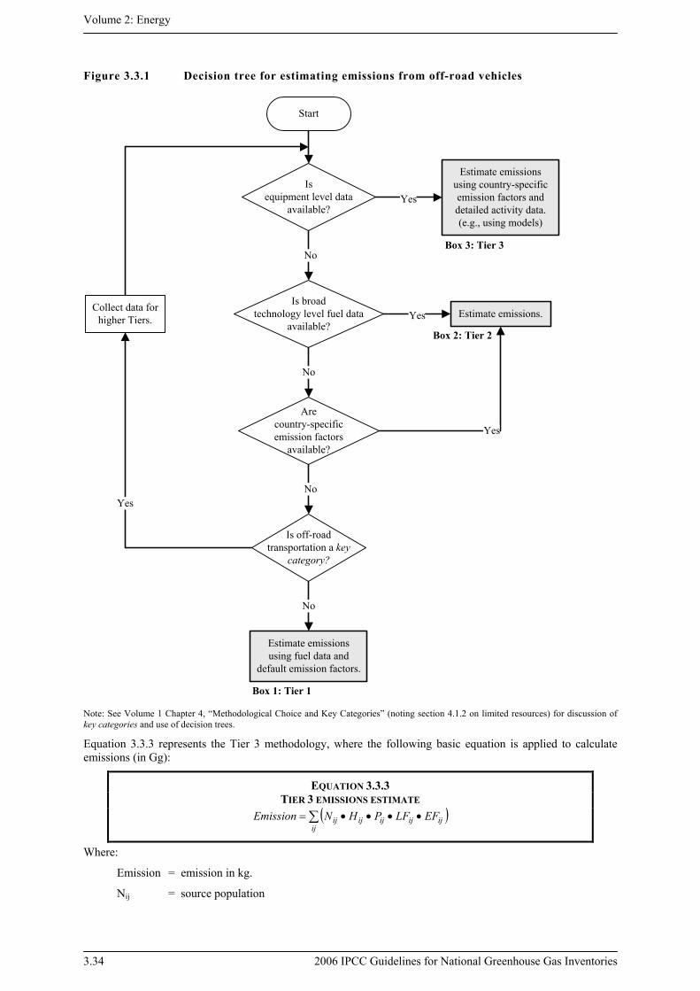
Volume 2: Energy
3.34 2006 IPCC Guidelines for National Greenhouse Gas Inventories
Figure 3.3.1 Decision tree for estimating emissions from off-road vehicles
Start
Isequipment level data
available?
Is off-roadtransportation a key
category?
Estimate emissionsusing country-specific emission factors and detailed activity data.(e.g., using models)
Yes
Yes
No
No
Estimate emissions.
Estimate emissionsusing fuel data and
default emission factors.
Box 2: Tier 2
Box 1: Tier 1
Box 3: Tier 3
Collect data for higher Tiers.
Arecountry-specificemission factors
available?
Is broadtechnology level fuel data
available?Yes
NoYes
No
Note: See Volume 1 Chapter 4, “Methodological Choice and Key Categories” (noting section 4.1.2 on limited resources) for discussion of key categories and use of decision trees.
Equation 3.3.3 represents the Tier 3 methodology, where the following basic equation is applied to calculate emissions (in Gg):
EQUATION 3.3.3 TIER 3 EMISSIONS ESTIMATE
( )∑ ••••=ij
ijijijijij EFLFPHNEmission
Where:
Emission = emission in kg.
Nij = source population

Chapter 3: Mobile Combustion
2006 IPCC Guidelines for National Greenhouse Gas Inventories 3.35
Hij = annual hours of use of vehicle i (h)
Pij = average rated power of vehicle i (kW)
LFij = typical load factor of vehicle i (fraction between 0 and 1)
EFij = average emission factor for use of fuel j in vehicle i (kg/kWh)
i = off-road vehicle type
j = fuel type
Equation 3.3.3 may be stratified by factors such as age, technological vintage or usage pattern, and this will increase the accuracy of the estimates provided self-consistent sets of parameters H, P, LF and EF are available to support the stratification, (EEA 2005). Other detailed modelling tools are available for estimating off-road emissions using Tier 3 methodology (e.g., NONROAD (USEPA 2005a) and COPERT (Ntziachristos 2000)).
For estimating CO2 emissions from use of urea-based additives in catalytic converters (non-combustive emissions), Equation 3.3.4 is used:
EQUATION 3.3.4 EMISSIONS FROM UREA-BASED CATALYTIC CONVERTERS
⎟⎠⎞
⎜⎝⎛••⎟
⎠⎞
⎜⎝⎛•=
1244
6012 FactorPurityActivityEmissions
Where:
Emission = Emission of CO2 (kg)
Activity = Mass (kg) of urea-based additive consumed for use in catalytic converters
Purity factor = Fraction of urea in the urea-based additive (if percent, divide by 100)
The factor (12/60) captures the stochiometric conversion from urea ((CO(NH2)2)) to carbon, while factor (44/12) converts carbon to CO2.
3.3.1.2 CHOICE OF EMISSION FACTORS Default CO2 emission factors assume that 100% of the fuel carbon is oxidised to CO2. This is irrespective of whether the carbon is emitted initially as CO2, CO, NMVOC or as particulate matter.
Country-specific NCV and CEF data should be used for Tiers 2 and 3. Inventory compilers may wish to consult CORINAIR 2004 or the EFDB for emission factors, noting that responsibility remains with the inventory compilers to ensure that emission factors taken from the EFDB are applicable to national circumstances.
For a Tier 3 approach example, please see Box 3.3.1 where more information on tailoring the NONROAD emissions model using country-specific data as well as the model to enhance national emission factors are given.
The default emission factors for CO2 and their uncertainty ranges, and the default emission factors for CH4 and N2O for Tier 1 are provided in Table 3.3.1. To estimate CO2 emissions, inventory compilers also have the option of using emission factors based on country-specific fuel consumption by off-road vehicles.

Volume 2: Energy
3.36 2006 IPCC Guidelines for National Greenhouse Gas Inventories
TABLE 3.3.1 DEFAULT EMISSION FACTORS FOR OFF-ROAD MOBILE SOURCES AND MACHINERY (a)
CO2 CH4(b) N2O (c)
Off-Road Source
Default (kg/TJ) Lower Upper Default
(kg/TJ) Lower Upper Default (kg/TJ) Lower Upper
Diesel Agriculture 74 100 72 600 74 800 4.15 1.67 10.4 28.6 14.3 85.8 Forestry 74 100 72 600 74 800 4.15 1.67 10.4 28.6 14.3 85.8 Industry 74 100 72 600 74 800 4.15 1.67 10.4 28.6 14.3 85.8 Household 74 100 72 600 74 800 4.15 1.67 10.4 28.6 14.3 85.8
Motor Gasoline 4-stroke Agriculture 69 300 67 500 73 000 80 32 200 2 1 6 Forestry 69 300 67 500 73 000 Industry 69 300 67 500 73 000 50 20 125 2 1 6 Household 69 300 67 500 73 000 120 48 300 2 1 6
Motor Gasoline 2-Stroke Agriculture 69 300 67 500 73 000 140 56 350 0.4 0.2 1.2 Forestry 69 300 67 500 73 000 170 68 425 0.4 0.2 1.2 Industry 69 300 67 500 73 000 130 52 325 0.4 0.2 1.2 Household 69 300 67 500 73 000 180 72 450 0.4 0.2 1.2 Source: EEA 2005. Note: CO2 emission factor values represent full carbon content. a Data provided in Table 3.3.1 are based on European off-road mobile sources and machinery. For gasoline, in case fuel consumption by sector is not discriminated, default values may be obtained according to national circumstances, e.g. prevalence of a given sector or weighting by activity b Including diurnal, soak and running losses. c In general, off-road vehicles do not have emission control catalysts installed (there may be exceptions among off-road vehicles in urban areas, such as ground support equipment used in urban airports and harbours). Properly operating catalysts convert nitrogen oxides to N2O and CH4 to CO2. However, exposure of catalysts to high-sulphur or leaded fuels, even once, causes permanent deterioration (Walsh, 2003). This effect, if applicable, should be considered when adjusting emission factors.
3.3.1.3 CHOICE OF ACTIVITY DATA Comprehensive top-down activity data on off-road vehicles are often unavailable, and where this is the case statistical surveys will be necessary to estimate the share of transport fuel used by off-road vehicles. Survey design is discussed in Chapter 2 of Vol.1 (Approaches to Data Collection). The surveys should be at the level of disaggregation indicated in Table 3.3.1 to make use of the default emission factor data, and be more detailed for the higher tiers. For the Tier 3 approach, modelling tools are available to estimate the amount of fuel consumed by each subcategory of equipment. Box 3.3.1 provides further information on using the NONROAD emissions model. This model may also be developed to incorporate country-specific modifications (see Box 3.3.2 for the Canadian experience).
Chapter 3: Mobile Combustion
2006 IPCC Guidelines for National Greenhouse Gas Inventories 3.37
BOX 3.3.1 NONROAD EMISSION MODEL (USEPA)
NONROAD 2005 is a mathematical model developed by the USEPA and may be used to estimate and forecast emissions from the non-road (off-road) transportation sectors. The model itself and all available supporting documentation are accessible on the EPA’s website (http://www.epa.gov/otaq/nonrdmdl.htm). This model estimates emissions for six exhaust gases: hydrocarbons (HC), NOX, carbon monoxide (CO), carbon dioxide (CO2), sulphur oxides (SOX), and particulate matter (PM). The user selects among five different types for reporting HC — as total hydrocarbons (THC), total organic gases (TOG), non-methane organic gases (NMOG), non-methane hydrocarbons (NMHC), and volatile organic compounds (VOC).
Generally, this model can perform a bottom-up estimation of emissions from the defined sources using equipment specific parameters such as: (i) engine populations; (ii) annual hours of use; (iii) power rating (horsepower); (iv) load factor (percent load or duty cycle), and (v) brake-specific fuel consumption (fuel consumed per horsepower-hour). The function will calculate the amount of fuel consumed by each subcategory of equipment. Subsequently, sub-sector (technology/fuel)-specific emission factors may then be applied to develop the emission estimate. The model is sensitive to the chosen parameters but may be used to apportion emissions estimates developed using a top-down approach.
It is not uncommon for the bottom-up approach using this model to deviate from a similar top-down result by a factor of 2 (100%) and therefore users are cautioned to review documentation for areas where this gap may be reduced through careful adjustment of their own inputs. Consequently, users must have some understanding of the population and fuel/technology make-up of the region being evaluated. However, reasonable adjustments can be established based upon: national manufacturing levels; importation/export records; estimated lifespan and scrappage functions. Scrappage functions attempt to define the attrition rate of equipment and may help illustrate present populations based upon historic equipment inventories (see Box 3.2.3 of Section 3.2 of this volume).
3.3.1.4 COMPLETENESS Duplication of off-road and road transport activity data should be avoided. Validation of fuel consumption should follow the principles outlined in Section 3.2.1.3. Lubricants should be accounted for based on their use in off-road vehicles. Lubricants that are mixed with motor gasoline and combusted should be included with fuel consumption data. Other uses of lubricants are covered in the Volume 3: IPPU Chapter 5).
Amounts of carbon from biomass, eg. biodiesel, oxygenates and some other blending agents should be estimated separately, and reported as an information item to avoid double counting as these emissions are already treated in the AFOLU sector.
3.3.1.5 DEVELOPING A CONSISTENT TIME SERIES It is good practice to determine activity data (e.g., fuel use) using the same method for all years. If this is not possible, data collection should overlap sufficiently in order to check for consistency in the methods employed. If it is not possible to collect activity data for the base year (e.g. 1990), it may be appropriate to extrapolate data backwards using trends in other activity data records.
Emissions of CH4 and N2O will depend on engine type and technology. Unless technology-specific emission factors have been developed, it is good practice to use the same fuel-specific set of emission factors for all years.
Mitigation activities resulting in changes in overall fuel consumption will be readily reflected in emission estimates if actual fuel activity data are collected. Mitigation options that affect emission factors, however, can only be captured by using engine-specific emission factors, or by developing control technology assumptions. Changes in emission factors over time should be well documented.
For more information on determining base year emissions and ensuring consistency in the time series, see Volume 1, Chapter 5 (Time Series Consistency).

Volume 2: Energy
3.38 2006 IPCC Guidelines for National Greenhouse Gas Inventories
BOX 3.3.2 CANADIAN EXPERIENCE WITH NONROAD MODEL
Using the model to enhance national emission factors:
NONROAD is initially populated with data native to the United States but may be customised for a given region or Party by simply adjusting the assumed input parameters to accommodate local situations. Parties may wish to designate their region as similar to one of those present in the USA to better emulate the seasonal climate. However, a designated temperature regime may also be input elsewhere. The NONROAD model is, thus, pre-loaded with local USA defaults thereby allowing their constituents to query it immediately.
Canada has begun to adjust this model by commencing national studies to better evaluate country-specific engine populations, available technologies, load factors and brake-specific fuel consumption values (BSFC) unique to the Canadian region. This new information will facilitate creation of Canada-specific input files and therefore not alter the core EPA programme algorithm but allow complete exploitation of the programmes strengths by providing more representative population and operating definitions. Through the introduction of lower uncertainty input data, the model may be used in conjunction with national fuel consumption statistics to arrive at a reasonable, disaggregated emission estimate. When operated with a similarly constructed On-Road model, for which operating parameters are better understood, a complete bottom-up, “apparent” fuel consumption estimate may be scaled to total national fuel sales. The country has used this modelling concept to help improve country-specific emission factors for the off-road consumption of fuel. The total fuel consumed is estimated by fuel type for each of the highly aggregated equipment sectors: (i) 2 cycle versus 4 cycle engines; (ii) Agriculture, Forestry, Industrial, Household and Recreational sub-sectors; (iii) gasoline versus diesel (spark vs. compression ignition). Once the model reports the total amount of fuels consumed according to this matrix, a composite emission factor is built based on the weighted averages of the contributing sub-sectors and their unique emission factors. The 2 cycle versus 4 cycle proportions will contribute to an average Off-Road gasoline EF while the Diesel EF is directly determined. Emission factors representing most GWP gases are not well researched and documented currently in North America and therefore, Canada has historically utilized applicable CORINAIR emission factors for these aggregated equipment sectors. The similarities between earlier technologies present in Europe and North America allow this utilization without introducing unreasonable uncertainty.
3.3.2 Uncertainty assessment Greenhouse gas emissions from off-road sources are typically much smaller than those from road transportation, but activities in this category are diverse and are thus typically associated with higher uncertainties because of the additional uncertainty in activity data.
The types of equipment and their operating conditions are typically more diverse than that for road transportation, and this may give rise to a larger variation in emission factors and thus to larger uncertainties. However, the uncertainty estimate is likely to be dominated by the activity data, and so it is reasonable to assume as a default that the values in section 3.2.1.2 apply. Also, emission controls, if installed, are likely to be inoperable due to catalyst failure (e.g., from exposure to high-sulphur fuel). Thus, N2O and CH4 emissions are more closely related to combustion-related factors such as fuel and engine technology than to emission control systems.
3.3.2.1 ACTIVITY DATA UNCERTAINTY Uncertainty in activity data is determined by the accuracy of the surveys or bottom-up models on which the estimates of fuel usage by off-road source and fuel type (see Table 3.3.1 for default classification) are based. This will be very case-specific, but factor of 2 uncertainties are certainly possible, unless if there is evidence to the contrary from the survey design.
3.3.3 Inventory Quality Assurance/Quality Control (QA/QC)
It is good practice to conduct quality control checks as outlined in Chapter 6 of Volume 1, and expert review of the emission estimates, plus additional checks if higher tier methods are used.

Chapter 3: Mobile Combustion
2006 IPCC Guidelines for National Greenhouse Gas Inventories 3.39
In addition to the guidance above, specific procedures of relevance to this source category are outlined below.
Review of emission factors
The inventory compiler should ensure that the original data source for national factors is applicable to each category and that accuracy checks on data acquisition and calculations have been performed. For default factors, the inventory compiler should ensure that the factors are applicable and relevant to the category. If possible, the default factors should be compared to national factors to provide further indication that the factors are applicable and reasonable.
Check of act iv ity data
The source of the activity data should be reviewed to ensure applicability and relevance to the category. Where possible, the data should be compared to historical activity data or model outputs to look for anomalies. Where surveys data have been used, the sum of on-road and off-road fuel usage should be consistent with total fuel used in the country. In addition, a completeness assessment should be conducted, as described in Section 3.3.1.4.
External review
The inventory compiler should carry out an independent, objective review of calculations, assumptions or documentation or both of the emissions inventory to assess the effectiveness of the QC programme. The peer review should be performed by expert(s) who are familiar with the source category and who understand national greenhouse gas inventory requirements.
3.3.4 Reporting and Documentation It is good practice to document and archive all information required to produce the national emissions inventory estimates as outlined in Chapter 8 of Volume 1.
It is not practical to include all documentation in the national inventory report. However, the inventory should include summaries of methods used and references to source data such that the reported emissions estimates are transparent and steps in their calculation may be retraced.
Some examples of specific documentation and reporting issues relevant to this source category are provided below.
In addition to reporting emissions, it is good practice to provide:
• Source of fuel and other data;
• Emission factors used and their associated references;
• Analysis of uncertainty or sensitivity of results or both to changes in input data and assumptions.
• Basis for survey design, where used to determine activity data
• References to models used in making the estimates
3.3.5 Reporting tables and worksheets See the four pages of the worksheets (Annex 1) for the Tier I Sectoral Approach which are to be filled in for each of the source categories. The reporting tables are available in Volume 1, Chapter 8.
3.4 RAILWAYS Railway locomotives generally are one of three types: diesel, electric, or steam. Diesel locomotives generally use diesel engines in combination with an alternator or generator to produce the electricity required to power their traction motors.
Diesel locomotives are in three broad categories – shunting or yard locomotives, railcars, and line haul locomotives. Shunting locomotives are equipped with diesel engines having a power output of about 200 to 2000 kW. Railcars are mainly used for short distance rail traction, e.g., urban/suburban traffic. They are equipped with a diesel engine having a power output of about 150 to 1000 kW. Line haul locomotives are used for long distance rail traction – both for freight and passenger. They are equipped with a diesel engine having a power output of about 400 to 4000 kW (EEA, 2005).

Volume 2: Energy
3.40 2006 IPCC Guidelines for National Greenhouse Gas Inventories
Electric locomotives are powered by electricity generated at stationary power plants as well as other sources. The corresponding emissions are covered under the Stationary Combustion Chapter of this Volume.
Steam locomotives are now generally used for very localized operations, primarily as tourist attractions and their contribution to greenhouse gas emissions is correspondingly small. However for a few countries, up to the 1990s, coal was used in a significant fraction of locomotives. For completeness, their emissions should be estimated using an approach similar to conventional steam boilers, which are covered in the Stationary Combustion Chapter.
3.4.1 Methodological issues Methodologies for estimating greenhouse gas emissions from railway vehicles (Section 3.4.1.1), have not changed fundamentally since the publication of the 1996 IPCC Guidelines and the GPG2000. However, for consistency with the Stationary Combustion Chapter, CO2 emissions are now estimated on the basis of the full carbon content of the fuel. This chapter covers good practice in the development of estimates for the direct greenhouse gases CO2, CH4 and N2O. For the precursor gases, or indirect greenhouse gases of CO, NMVOCs, SO2, PM, and NOx, please refer to the EMEP/Corinair Guidebook (EEA, 2005) for other mobile sources).
3.4.1.1 CHOICE OF METHOD There are three methodological options for estimating CO2, CH4, and N2O emissions from railways. The decision trees in Figures 3.4.1 and 3.4.2 give the criteria for choosing methodologies.
Figure 3.4.1 Decision tree for estimating CO2 emissions from railways
Start
AreCountry-specific data
on fuel carbon contents available?
Calculate emissionsusing Eq. 3.4.1.Yes
No
Calculate emissions usingEq. 3.4.1 and default
emission factors.
Box 2: Tier 1
Box 1: Tier 2
Collect country-specific data on fuel
carbon contents.
Is this akey category? Yes
No
Note: See Volume 1 Chapter 4, “Methodological Choice and Key Categories” (noting section 4.1.2 on limited resources) for discussion of key categories and use of decision trees.

Chapter 3: Mobile Combustion
2006 IPCC Guidelines for National Greenhouse Gas Inventories 3.41
Figure 3.4.2 Decision tree for estimating CH4 and N2O emissions from railways
Start
Islocomotive-specific
activity data and emissionfactor available?
Calculate emissions using detailed model and emission factors.
Yes
No
Calculate emissionsusing Eq. 3.4.1.
Box 1: Tier 1
Box 3: Tier 3
Estimate fuel consumptionby locomotive type,
and/or country- specificemission factors.
Are fuelstatistics by locomotive type
available?Yes
No
Is this akey category?
Box 2: Tier 2
Yes
No
Calculate emissionsusing Eq. 3.4.2.
Note: See Volume 1 Chapter 4, “Methodological Choice and Key Categories” (noting section 4.1.2 on limited resources) for discussion of key categories and use of decision trees.
The three tiers of estimation methodologies are variations of the same fundamental equation:
EQUATION 3.4.1 GENERAL METHOD FOR EMISSIONS FROM LOCOMOTIVES
( )∑ •=j
jj EFFuelEmissions
Where:
Emissions = emissions (kg)
Fuel j = fuel type j consumed (as represented by fuel sold) in (TJ)
EF j = emission factor for fuel type j, (kg/TJ)
j = fuel type
For Tier 1, emissions are estimated using fuel-specific default emission factors as listed in Table 3.4.1, assuming that for each fuel type the total fuel is consumed by a single locomotive type. For CO2, Tier 2 uses equation 3.4.1 again with country-specific data on the carbon content of the fuel. There is little or no advantage in going beyond Tier 2 for estimating CO2 emissions.
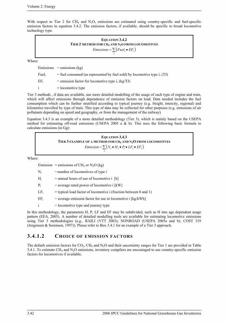
Volume 2: Energy
3.42 2006 IPCC Guidelines for National Greenhouse Gas Inventories
With respect to Tier 2 for CH4 and N2O, emissions are estimated using country-specific and fuel-specific emission factors in equation 3.4.2. The emission factors, if available, should be specific to broad locomotive technology type.
EQUATION 3.4.2 TIER 2 METHOD FOR CH4 AND N2O FROM LOCOMOTIVES
( )∑ •=i
ii EFFuelEmissions
Where:
Emissions = emissions (kg)
Fueli = fuel consumed (as represented by fuel sold) by locomotive type i, (TJ)
EFi = emission factor for locomotive type i, (kg/TJ)
i = locomotive type
Tier 3 methods , if data are available, use more detailed modelling of the usage of each type of engine and train, which will affect emissions through dependence of emission factors on load. Data needed includes the fuel consumption which can be further stratified according to typical journey (e.g. freight, intercity, regional) and kilometres travelled by type of train. This type of data may be collected for other purposes (e.g. emissions of air pollutants depending on speed and geography, or from the management of the railway).
Equation 3.4.3 is an example of a more detailed methodology (Tier 3), which is mainly based on the USEPA method for estimating off-road emissions (USEPA 2005 a & b). This uses the following basic formula to calculate emissions (in Gg):
EQUATION 3.4.3 TIER 3 EXAMPLE OF A METHOD FOR CH4 AND N2O FROM LOCOMOTIVES
( )∑ ••••=i
iiiii EFLFPHNEmission
Where:
Emission = emissions of CH4 or N2O (kg)
Ni = number of locomotives of type i
Hi = annual hours of use of locomotive i [h]
Pi = average rated power of locomotive i [kW]
LFi = typical load factor of locomotive i (fraction between 0 and 1)
EFi = average emission factor for use in locomotive i [kg/kWh]
i = locomotive type and journey type
In this methodology, the parameters H, P, LF and EF may be subdivided, such as H into age dependent usage pattern (EEA, 2005). A number of detailed modelling tools are available for estimating locomotive emissions using Tier 3 methodologies (e.g., RAILI (VTT 2003); NONROAD (USEPA 2005a and b); COST 319 (Jorgensen & Sorenson, 1997)). Please refer to Box 3.4.1 for an example of a Tier 3 approach.
3.4.1.2 CHOICE OF EMISSION FACTORS The default emission factors for CO2, CH4 and N2O and their uncertainty ranges for Tier 1 are provided in Table 3.4.1. To estimate CH4 and N2O emissions, inventory compilers are encouraged to use country-specific emission factors for locomotives if available.

Chapter 3: Mobile Combustion
2006 IPCC Guidelines for National Greenhouse Gas Inventories 3.43
TABLE 3.4.1 DEFAULT EMISSION FACTORS FOR THE MOST COMMON FUELS USED FOR RAIL TRANSPORT
Gas Diesel (kg/TJ) Sub-bituminous Coal (kg/TJ)
Default Lower Upper Default Lower Upper
CO2 74 100 72 600 74 800 96 100 72 800 100 000
CH4 1 4.15 1.67 10.4 2 0.6 6
N2O 1 28.6 14.3 85.8 1.5 0.5 5
Notes: 1 For an average fuel consumption of 0.35 litres per bhp-hr (break horse power-hour) for a 4000 HP locomotive, (0.47 litres per kWh for a 2983 kW locomotive).(Dunn, 2001). 2 The emission factors for diesel are derived from (EEA, 2005) (Table 8-1), while for coal from Table 2.2 of the Stationary Combustion chapter.
These default emission factors may, for non-CO2 gases, be modified depending on the engine design parameters in accordance with Equation 3.4.4, using pollutant weighing factors in Table 3.4.2
EQUATION 3.4.4 WEIGHTING OF CH4 AND N2O EMISSION FACTORS FOR SPECIFIC TECHNOLOGIES
dieseldefaultidieseli EFPWFEF ,, •=
Where:
EFi,diesel = engine specific emission factor for locomotive of type i (kg/TJ)
PWFi = pollutant weighing factor for locomotive of type i [dimensionless]
EFdefault,diesel = default emission factor for diesel (applies to CH4, N2O) (kg/TJ)
TABLE 3.4.2 POLLUTANT WEGHTING FACTORS AS FUNCTIONS OF ENGINE DESIGN PARAMETERS FOR UNCONTROLLED
ENGINES(DIMENSIONLESS)
Engine type CH4 N2O
Naturally Aspirated Direct Injection 0.8 1.0
Turbo-Charged Direct Injection / Inter-cooled Turbo-Charged Direct Injection 0.8 1.0
Naturally Aspirated Pre-chamber Injection 1.0 1.0
Turbo-Charged Pre-chamber Injection 0.95 1.0
Inter-cooled Turbo-Charged Pre-chamber Injection 0.9 1.0
Source: EEA 2005 (Table 8-9);
To take into account the increase in CH4 and N2O emissions with the age, the default emission factors for CH4 may be increased by 1.5 percent per year while deterioration for N2O is negligible (EEA, 2005).

Volume 2: Energy
3.44 2006 IPCC Guidelines for National Greenhouse Gas Inventories
3.4.1.3 CHOICE OF ACTIVITY DATA National level fuel consumption data are needed for estimating CO2 emissions for Tier 1 and Tier 2 approaches. For estimating CH4 and N2O emissions using Tier 2, locomotive category level data is needed. Tier 3 approaches require activity data for operations (for example gross tonne kilometre (GTK) and duty cycles) at specific line haul locomotive level. These methods also require other locomotive-specific information, such as source population (with age and power ranges), mileage per train tonnage, annual hours of use and age-dependent usage patterns, average rated horse power (with individual power distribution within given power ranges), load factor, section information (such as terrain topography and train speeds). There are alternate modelling approaches for Tier 3 estimation (VTT 2003; EEA 2005).
The railway or locomotive companies, or the relevant transport authorities may be able to provide fuel consumption data for the line haul and yard locomotives. The contribution from yard locomotives is likely to be very small for almost all countries. If the annual fuel consumption is not provided separately for yard locomotives, it may be possible to estimate fuel use if typical data on their use and daily fuel use is available according to the following equation:
BOX 3.4.1 EXAMPLE OF TIER 3 APPROACH
The 1998 EPA non-road diesel engine regulations are structured as a 3-tiered progression (USEPA, 1998). Each USEPA-tier involves a phase in (by horse power rating) over several years. USEPA-Tier 0 standards were in phase until 2001. The more stringent USEPA-Tier 1 standards took effect from 2002 to 2004, and yet more stringent USEPA-Tier 2 standards phase-in from 2005 and beyond. The main improvements are in the NOx and PM emissions over the USEPA-tiers. Use of improved diesel with lower sulphur content contributes to reduced SO2 emissions. The table below provides broad technology level emission factors for these and other locomotives above 3000 HP. Emission factors may also be provided in g/passenger-kilometer for passenger trains and g/ton-kilometer for freight trains for higher tiers if country-specific information is available (e.g., Hahn, 1989; UNECE 2002).
BROAD TECHNOLOGY LEVEL EMISSION FACTORS
Power Reported emission levels (g/kWh) Model Engine
HP kW
Brake specific diesel fuel
consumption (kg/kWh) NOx CO HC CO2
EMD SD-40 645E3B 3000 2237 0.246 15.82 2.01 0.36 440
EMD SD-60 710G3 3800 2834 0.219 13.81 2.68 0.35 391 EMD SD-70 710G3C 4000 2983 0.213 17.43 0.80 0.38 380
EMD SD-75 710G3EC 4300 3207 0.206 17.84 1.34 0.40 367
GE Dash 8 7FDL 3800 2834 0.219 16.63 6.44 0.64 391
GE Dash 9 7FDL 4400 3281 0.215 15.15 1.88 0.28 383
GE Dash 9 7FDL (Tier 0) 4400 3281 0.215 12.74 1.88 0.28 383
Evolution GEVO 12 4400 3281 NA 10.86 1.21 0.40 NA
2ТЕ116 1А-5Д49 6035 2●2250 0.214 16.05 10.70 4.07 382
2ТЕ10М 10Д100 5900 2●2200 0.226 15.82 10.62 4.07 403
ТЕП60 11Д45 2950 2200 0.236 16.05 10.62 3.84 421 ТЕП70 2А-5Д49 3420 2550 0.211 15.83 10.55 4.01 377
2М62 14Д40 3943 2●1470 0.231 13.40 9.01 3.23 412 Sources: 1 EMD and GE locomotive information based on Dunn, 2001. Lower tier CO and HC estimates for line-haul locomotives are 6.7 g/kWh and 1.3 g/kWh respectively. 2 For the TE models and 2M62, estimations are based on GSTU 1994.
Chapter 3: Mobile Combustion
2006 IPCC Guidelines for National Greenhouse Gas Inventories 3.45
EQUATION 3.4.5 ESTIMATING YARD LOCOMOTIVE FUEL CONSUMPTION
Inventory fuel consumption = Number of yard locomotives • Average fuel consumption per locomotive and day • Average number of days of operation per locomotive in the year
The number of yard locomotives can be obtained from railway companies or transport authorities. If average fuel consumption per day is unknown, a value of 863 litres per day can be used (USEPA, 2005a). The number of days of operation is usually 365. If data for the number of yard locomotives cannot be obtained, the emissions inventory can be approximated by assuming that all fuel is consumed by line haul locomotives.
If fuel consumption data are available for the jurisdiction (State or Territory) as a whole, double counting may occur when locomotives of one company fill-in the jurisdiction of another company. This can be resolved at higher Tiers by the use of operating data.
Where higher tier approaches are used, care should be taken that the fuel consumption data used for CO2 is consistent with the activity data used for CH4 and N2O.
3.4.1.4 COMPLETENESS Diesel fuel is the most common fuel type used in railways, but inventory compilers should be careful not to omit or double count the other fuels that may be used in diesel locomotives for traction purposes. These may be mixed with diesel and may include petroleum fuels (such as residual fuel, fuel oils, or other distillates), bio-diesel (e.g. oil esters from rape seed, soy bean, sunflower, Jatropha, or Karanjia oil, or recovered vegetable and animal fats), and synthetic fuels. Bio-diesel can be used in all diesel engines with slight or no modification. Blending with conventional diesel is possible. Synthetic fuels include synthetic middle distillates (SMD) and Dimethyl Ether (DME) to be produced from various carbonaceous feedstocks, including natural gas, residual fuel oil, heavy crude oils, and coal via the production of synthesis gas. The mix varies and presently it is between 2 to 5 percent bio-diesel and the remaining petroleum diesel. The emission properties of these fuels are considered to be similar to those used for the road transport sector. CO2 emissions from fuels derived from biomass should be reported as information items, and not included in the national total to avoid double counting.
Diesel locomotives may combust natural gas or coal for heating cars. Although these energy sources may be “mobile,” the methods for estimating emissions from combustion of fuels for heat are covered under the Stationary Combustion section of this Energy Volume. Inventory compilers should be careful not to omit or double count the emissions from energy used for carriage heating in railways.
Diesel locomotives also consume significant amounts of lubricant oils. The related emissions are dealt with in Chapter 5 of the IPPU volume.
There are potential overlaps with other source sectors. A lot of statistical data will not include fuel used in other activities such as stationary railway sources; off-road machinery, vehicles and track machines in railway fuel use. Their emissions should not be included here but in the relevant non-railway categories as stationary sources, off-road etc. If this is not the case and it is impossible to separate these other uses from the locomotives, then it is good practice to note this in any inventory report or emission reporting tables.
3.4.1.5 DEVELOPING A CONSISTENT TIME SERIES Emissions of CH4 and N2O will depend on engine type and technology. Unless technology-specific emission factors have been developed, it is good practice to use the same fuel-specific set of emission factors for all years.
Mitigation options that affect emission factors can only be captured by using engine-specific emission factors, or by developing control technology assumptions. These changes should be adequately documented.
For more information on determining base year emissions and ensuring consistency in the time series, see Chapter 5 of Volume 1: Time Series Consistency.
3.4.1.6 UNCERTAINTY ASSESSMENT Greenhouse gas emissions from railways are typically much smaller than those from road transportation because the amounts of fuel consumed are less, and also because operations often occur on electrified lines, in which case the emissions associated with railway energy use will be reported under power generation and will depend on the characteristics of that sector.

Volume 2: Energy
3.46 2006 IPCC Guidelines for National Greenhouse Gas Inventories
To reduce uncertainty, a comprehensive approach is needed for both emission factors and activity data, especially where bottom-up activity data are used. The use of representative locally estimated data is likely to improve accuracy although uncertainties may remain large. It is good practice to document the uncertainties both in the emission factors as well as in the activity data. Further guidance on uncertainty estimates for emission factors can be found in Chapter 3 of Volume 1: Uncertainties.
Emission factor uncertainty
Table 3.4.1 provides ranges indicating the uncertainties associated with diesel fuel. In the absence of specific information, the percentage relationship between the upper and lower limiting values and the central estimate may be used to derive default uncertainty ranges associated with emission factors for additives.
Activity data uncertainty
The uncertainty in top-down activity data (fuel use) is likely to be of the order 5 percent. The uncertainty in disaggregated data for bottom-up estimates (usage or fuel use by type of train) is unlikely to be less than 10 percent and could be several times higher, depending on the quality of the underlying statistical surveys. Bottom-up estimates are however necessary for estimating non-CO2 gases at higher tiers. These higher tier calculations could also yield CO2 estimates, but these will probably be more uncertain than Tier 1 or 2. Thus the way forward where railways are a key category is to use the top-down estimate for CO2 with country-specific fuel carbon contents, and higher tier estimates for the other gases. A bottom-up CO2 estimate can then be used for QA/QC cross-checks.
Further guidance on uncertainty estimates for activity data can be found in Chapter 3 of Volume 1: Uncertainties.
3.4.2 Inventory Quality Assurance/Quality Control (QA/QC)
It is good practice to conduct quality control checks as outlined in Chapter 6 of Volume 1: Quality Assurance/ Quality Control and Verification.
Additional quality control checks as outlined in Tier 2 procedures in Chapter 6 of Volume 1 may also be applicable, particularly if higher tier methods are used to determine emissions from this source category. Inventory compilers are encouraged to use higher tier QA/QC for key categories as identified in Chapter 4 of Volume 1: Methodological Choice and Identification of Key Categories. In addition to the above guidance, specific procedures of relevance to this source category are outlined below.
Review of emission factors
The inventory compiler should ensure that the original data source for national factors is applicable to each category and that accuracy checks on data acquisition and calculations have been performed. For the IPCC default factors, the inventory compiler should ensure that the factors are applicable and relevant to the category. If possible, the IPCC default factors should be compared to national factors to provide further indication that the factors are applicable and reasonable.
Check of activity data
The source of the activity data should be reviewed to ensure applicability and relevance to the category. Where possible, the data should be compared to historical activity data or model outputs to look for anomalies. Data could be checked with productivity indicators such as fuel per unit of distance railway performance (freight and passenger kilometres) compared with other countries and compared across different years.
3.4.3 Reporting and Documentation It is good practice to document and archive all information required to produce the national emissions inventory estimates as outlined in Chapter 8 of Volume 1: Reporting Guidance and Tables.
In addition to reporting emissions, it is good practice to provide:
• the way in which detailed information needed for bottom-up estimates has been obtained, and what uncertainties are to be estimated;
• how any bottom-up method of fuel use has been reconciled with top-down fuel use statistics.
• emission factors used and their associated references, especially for additives
• the way in which any biofuel components have been identified.

Chapter 3: Mobile Combustion
2006 IPCC Guidelines for National Greenhouse Gas Inventories 3.47
The possible inclusion of fuels used for non-locomotive uses (see section 3.4.1.2 above).
3.4.4 Reporting tables and worksheets See the four pages of the worksheets (Annex 1) for the Tier I Sectoral Approach which are to be filled in for each of the source categories. The reporting tables are available in Volume 1, Section 8.
3.5 WATER-BORNE NAVIGATION This source category covers all water-borne transport from recreational craft to large ocean-going cargo ships that are driven primarily by large, slow and medium speed diesel engines and occasionally by steam or gas turbines. It includes hovercraft and hydrofoils. Water-borne navigation causes emissions of carbon dioxide (CO2), methane (CH4) and nitrous oxide (N2O), as well as carbon monoxide (CO), non-methane volatile organic compounds (NMVOCs), sulphur dioxide (SO2), particulate matter (PM) and oxides of nitrogen (NOx).
Section 3.5.5 contains definitions of specialist terms that may be useful to an inventory compiler.
3.5.1 Methodological issues This section deals with the direct greenhouse gases CO2, CH4, and N2O. The source category is set out in detail in Table 3.5.1. The methods discussed can be used also to estimate emissions from military water-borne navigation (see section 3.5.1.4). For the purpose of the emissions inventory, a distinction is made between domestic and international water-borne navigation. Any fugitive emissions from the transport of fossil fuels (e.g., by tanker) should be estimated and reported under the category “Fugitive emissions” as set out in Chapter 4 of this Volume.
3.5.1.1 CHOICE OF METHOD Two methodological tiers for estimating emissions of CO2, CH4, and N2O from water-borne navigation are presented. Both tiers apply emission factors to fuel consumption activity data. The decision tree shown in Figure 3.5.1 helps in making a choice between the two tiers. Emissions are estimated separately for domestic and international water-borne navigation.
Tier 1
The Tier 1 method is the simplest and can be applied with either default values or country-specific information. The fuel consumption data and emission factors in the Tier 1 method are fuel-type-specific and should be applied to the corresponding activity data (e.g. gas/diesel oil used for navigation). The calculation is based on the amount of fuel combusted and on emission factors for CO2, CH4, and N2O. The calculation is shown in Equation 3.5.1 and emission factors are provided in Table 3.5.2 and Table 3.5.3
EQUATION 3.5.1 WATER-BORNE NAVIGATION EQUATION
)( abab FactorEmissionConsumedFuelEmissions •= ∑
Where:
a = fuel type (diesel, gasoline, LPG, bunker, etc.)
b = water-borne navigation type (i.e., ship or boat, and possibly engine type.) (Only at Tier 2 is the fuel used differentiated by type of vessel so b can be ignored at Tier 1)
Tier 2
The Tier 2 method also uses fuel consumption by fuel type, but requires country-specific emission factors with greater specificity in the classification of modes (e.g. ocean-going ships and boats), fuel type (e.g. fuel oil), and even engine type (e.g. diesel) (Equation 3.5.1). In applying Tier 2, the inventory compilers should note that the EMEP/Corinair emission inventory guidebook (EEA, 2005) offers a detailed methodology for estimating ship emissions based on engine and ship type and ship movement data. The ship movement methodology can be used when detailed ship movement data and technical information on the ships are both available and can be used to differentiate emissions between domestic and international water-borne navigation.

Volume 2: Energy
3.48 2006 IPCC Guidelines for National Greenhouse Gas Inventories
TABLE 3.5.1 SOURCE CATEGORY STRUCTURE
Source category Coverage
1 A 3 d Water-borne Navigation
Emissions from fuels used to propel water-borne vessels, including hovercraft and hydrofoils, but excluding fishing vessels. The international/domestic split should be determined on the basis of port of departure and port of arrival, and not by the flag or nationality of the ship.
1 A 3 d i International Water-borne Navigation (International bunkers)
Emissions from fuels used by vessels of all flags that are engaged in international water-borne navigation. The international navigation may take place at sea, on inland lakes and waterways and in coastal waters. Includes emissions from journeys that depart in one country and arrive in a different country. Exclude consumption by fishing vessels (see Other Sector - Fishing). Emissions from international military water-borne navigation can be included as a separate sub-category of international water-borne navigation provided that the same definitional distinction is applied and data are available to support the definition.
1 A 3 d ii Domestic Water-borne Navigation
Emissions from fuels used by vessels of all flags that depart and arrive in the same country (exclude fishing, which should be reported under 1 A 4 c iii, and military, which should be reported under 1 A 5 b). Note that this may include journeys of considerable length between two ports in a country (e.g. San Francisco to Honolulu).
1 A 4 c iii Fishing (mobile combustion)
Emissions from fuels combusted for inland, coastal and deep-sea fishing. Fishing should cover vessels of all flags that have refuelled in the country (include international fishing).
1 A 5 b Mobile (water-borne navigation component)
All remaining water-borne mobile emissions from fuel combustion that are not specified elsewhere. Includes military water-borne navigation military emissions from fuel delivered to the country’s military not otherwise included separately in 1 A3 d i as well as fuel delivered within that country but used by the militaries of external countries that are not engaged in multilateral operations.
Multilateral operations (water-borne navigation component)
Emissions from fuels used for water-borne navigation in multilateral operations pursuant to the Charter of the United Nations. Include emissions from fuel delivered to the military in the country and delivered to the military of other countries.

Chapter 3: Mobile Combustion
2006 IPCC Guidelines for National Greenhouse Gas Inventories 3.49
Figure 3.5.1 Decision tree for emissions from water-borne navigation
Start
Are fuelconsumption data availableby fuel type for water-borne
navigation?
Estimate emissionsusing Tier 2 with
country-specific carbon content factors and
engine-specificCH4 and N2O
emission factors.
No
Yes
Estimate CO2 emissions using IPCC default carbon contents;
estimate CH4 and N2O emissionsusing IPCC default emission factors.
Box 3
Box 1
Develop statistics basedon other information
or proxy data.
Have thedata been differentiatedbetween international
and domestic?No
Yes
Arenational carbon
content dataavailable?
Box 2
Yes
No
Use Tier 2 for CO2 withcountry-specific carbon
contents and a Tier 1 for CH4and N2O with IPCC default
emission factors.
Arefuel-use data and
CH4 and N2O emission factors by engine type
available?
Is thisa key sourcecategory?
Collect data or estimateusing proxy data.
Yes
No
No
Initiate datacollection.
Yes
Note: See Volume 1 Chapter 4, “Methodological Choice and Key Categories” (noting section 4.1.2 on limited resources) for discussion of key categories and use of decision trees.
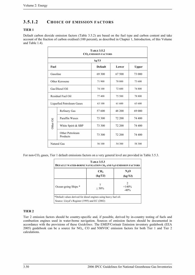
Volume 2: Energy
3.50 2006 IPCC Guidelines for National Greenhouse Gas Inventories
3.5.1.2 CHOICE OF EMISSION FACTORS
TIER 1
Default carbon dioxide emission factors (Table 3.5.2) are based on the fuel type and carbon content and take account of the fraction of carbon oxidised (100 percent), as described in Chapter 1, Introduction, of this Volume and Table 1.4).
TABLE 3.5.2 CO2 EMISSION FACTORS
kg/TJ
Fuel Default Lower Upper
Gasoline 69 300 67 500 73 000
Other Kerosene 71 900 70 800 73 600
Gas/Diesel Oil 74 100 72 600 74 800
Residual Fuel Oil 77 400 75 500 78 800
Liquefied Petroleum Gases 63 100 61 600 65 600
Refinery Gas 57 600 48 200 69 000
Paraffin Waxes 73 300 72 200 74 400
White Spirit & SBP 73 300 72 200 74 400
Oth
er O
il
Other Petroleum Products 73 300 72 200 74 400
Natural Gas 56 100 54 300 58 300
For non-CO2 gases, Tier 1 default emissions factors on a very general level are provided in Table 3.5.3.
TABLE 3.5.3 DEFAULT WATER-BORNE NAVIGATION CH4 AND N2O EMISSION FACTORS
CH4 (kg/TJ)
N2O
(kg/TJ)
Ocean-going Ships * 7 + 50%
2 +140% -40%
*Default values derived for diesel engines using heavy fuel oil. Source: Lloyd’s Register (1995) and EC (2002)
TIER 2
Tier 2 emission factors should be country-specific and, if possible, derived by in-country testing of fuels and combustion engines used in water-borne navigation. Sources of emission factors should be documented in accordance with the provisions of these Guidelines. The EMEP/Corinair Emission inventory guidebook (EEA 2005) guidebook can be a source for NOx, CO and NMVOC emission factors for both Tier 1 and Tier 2 calculations.

Chapter 3: Mobile Combustion
2006 IPCC Guidelines for National Greenhouse Gas Inventories 3.51
3.5.1.3 CHOICE OF ACTIVITY DATA Data on fuel consumption by fuel type and engine type (for N2O and CH4) are required to estimate emissions from water-borne navigation. In addition, in the current reporting procedures, emissions from domestic water-borne navigation are reported separately from international water-borne navigation which requires disaggregating the activity data to this level. For consistency, it is good practice to use similar definitions of domestic and international activities for aviation and water-borne navigation. These definitions are presented in Table 3.5.4 and are independent of the nationality or flag of the carrier. In some cases, the national energy statistics may not provide data consistent with this definition. It is good practice that countries separate the activity data consistent with this definition. In most countries, tax and custom dues are levied on bunkers for domestic consumption, and bunkers for international consumption are free of such dues. In the absence of more direct sources of data, information about domestic taxes may be used to distinguish between domestic and international fuel consumption. In any case, a country must clearly define the methodologies and assumptions used13.
TABLE 3.5.4 CRITERIA FOR DEFINING INTERNATIONAL OR DOMESTIC WATER-BORNE NAVIGATION (APPLIES TO EACH
SEGMENT OF A VOYAGE CALLING AT MORE THAN TWO PORTS) *
Journey type between two ports Domestic International
Departs and arrives in same country Yes No
Departs from one country and arrives in another No Yes * Most shipping movement data are collected on the basis of individual trip segments (from one departure to
the next arrival) and do not distinguish between different types of intermediate stop (as called for in GPG 2000). Basing the distinction on individual segment data is therefore simpler and is likely to reduce uncertainties. It is very unlikely that this change would make a significant change to the emission estimates. This does not change the way in which emissions from international journeys are reported as an information item and not included in national totals.
Fuel use data may be obtained using several approaches. The most feasible approach will depend on the national circumstances, but some of the options provide more accurate results than others. Several likely sources of actual fuel or proxy data are listed below, in order of typically decreasing reliability:
• National energy statistics from energy or statistical agencies;
• International Energy Agency (IEA) statistical information;
• Surveys of shipping companies (including ferry and freight);
• Surveys of fuel suppliers (e.g. quantity of fuels delivered to port facilities);
• Surveys of individual port and marine authorities;
• Surveys of fishing companies;
• Equipment counts, especially for small gasoline powered fishing and pleasure craft;
• Import/export records;
• Ship movement data and standard passenger and freight ferry schedules;
• Passenger counts and cargo tonnage data;
• International Maritime Organisation (IMO), engine manufacturers, or Jane's Military Ships Database;
• Ship movement data derived from Lloyds Register data
It may be necessary to combine and compare these data sources to get full coverage of shipping activities.
Marine diesel engines are the main power unit used within the marine industry for both propulsion and auxiliary power generation. Some vessels are powered by steam plants (EEA 2005). Water-borne navigation should also account for the fuel that may be used in auxiliary engines powering for example refrigeration plants and cargo 13
It is good practice to clearly state the reasoning and justification if any country opts to use the GPG2000 definitions.

Volume 2: Energy
3.52 2006 IPCC Guidelines for National Greenhouse Gas Inventories
pumps, and in boilers aboard vessels. Many steam powered oil tankers are still in operation, which consume more fuel per day when discharging their cargo in a port to operate the pumps than they do in deep sea steaming. Table 3.5.5 presents the average percentage of fuel consumed by both the main engines and auxiliary engines of the total fuel consumed by water-borne navigation vessel types. This allows the inventory compiler to apply the appropriate emissions factors, if available, as these factors may differ between main engines and auxiliary engines. Table 3.5.6 provides fuel consumption factors for various water-borne navigation vessel types, if the ship fleet by tonnage and category is collected.
TABLE 3.5.5 AVERAGE FUEL CONSUMPTION PER ENGINE TYPE (SHIPS >500 GRT)
Ship Type Main Engine Consumption
(%)
Avg. Number of Aux. Engines Per Vessel
Aux. Engine Consumption
(%)
Bulk Carriers 98% 1.5 2%
Combination Carriers 99% 1.5 1%
Container Vessels 99% 2 1%
Dry Cargo Vessels 95% 1.5 5%
Offshore Vessels 98% 1 2%
Ferries/Passenger Vessels 98% 2 2%
Reefer Vessels 97% 2 3%
RoRo Vessels 99% 1.5 1%
Tankers 99% 1.5 1%
Miscellaneous Vessels 98% 1 2%
Totals 98% 2%
Source: Fairplay Database of Ships, 2004. GRT = Gross Registered Tonnage
TABLE 3.5.6 FUEL CONSUMPTION FACTORS, FULL POWER
Ship type Average Consumption
(tonne/day)
Consumption at full power(tonne/day) as a function of gross tonnage(GRT)
Bulk Carriers
Solid Bulk 33.8 20.186 + 0.00049*GRT
Liquid Bulk 41.8 14.685 + 0.00079*GRT
General Cargo 21.3 9.8197 + 0.00143*GRT
Container 65.9 8.0552 + 0.00235*GRT
Passenger/Ro-Ro/Cargo 32.3 12.834 + 0.00156*GRT
Passenger 70.2 16.904 + 0.00198*GRT
High Speed Ferry 80.4 39.483 + 0.00972*GRT
Inland Cargo 21.3 9.8197 + 0.00143*GRT
Sail Ships 3.4 0.4268 +0.00100*GRT
Tugs 14.4 5.6511 +0.01048*GRT
Fishing 5.5 1.9387 +0.00448*GRT
Other Ships 26.4 9.7126 +0.00091*GRT
All Ships 32.8 16.263 + 0. 001*GRT
Source: Techne (1997)
Chapter 3: Mobile Combustion
2006 IPCC Guidelines for National Greenhouse Gas Inventories 3.53
In addition, although gases from cargo boil-off (primarily LNG or VOC recovery) may be used as fuels on ships, the amounts are usually not large in comparison to the total fuel consumed. Due to the small contribution, it is not required to account for this in the inventory.
3.5.1.4 MILITARY The 2006 IPCC Guidelines do not provide a distinct method for calculating military water-borne emissions. Emissions from military water-borne fuel use can be estimated using the equation 3.5.1 and the same calculation approach is recommended for non-military shipping. Due to the special characteristics of the operations, situations, and technologies (e.g., .aircraft carriers, very large auxiliary power plants, and unusual engine types) associated with military water-borne navigation, a more detailed method of data analysis is encouraged when data are available. Inventory compilers should therefore consult military experts to determine the most appropriate emission factors for the country’s military water-borne navigation.
Due to confidentiality issues (see completeness and reporting), many inventory compilers may have difficulty obtaining data for the quantity of military fuel use. Military activity is defined here as those activities using fuel purchased by or supplied to military authorities in the country. It is good practice to apply the rules defining civilian domestic and international operations in water-borne navigation to military operations when the data necessary to apply those rules are comparable and available. Data on military fuel use should be obtained from government military institutions or fuel suppliers. If data on fuel split are unavailable, all the fuel sold for military activities should be treated as domestic.
Emissions resulting from multilateral operations pursuant to the Charter of the United Nations should not be included in national totals, but reported separately; other emissions related to operations shall be included in the national emissions totals of one or more Parties involved. The national calculations should take into account fuel delivered to the country’s military, as well as fuel delivered within that country but used by the military of other countries. Other emissions related to operations (e.g., off-road ground support equipment) should be included in the national emissions totals in the appropriate source category.
3.5.1.5 COMPLETENESS For water-borne navigation emissions, the methods are based on total fuel use. Since countries generally have effective accounting systems to measure total fuel consumption. The largest area of possible incomplete coverage of this source category is likely to be associated with misallocation of navigation emissions in another source category. For instance, for small watercraft powered by gasoline engines, it may be difficult to obtain complete fuel use records and some of the emissions may be reported as industrial (when industrial companies use small watercraft), other off-road mobile or stationary power production. Estimates of water-borne emissions should include not only fuel for marine shipping, but also for passenger vessels, ferries, recreational watercraft, other inland watercraft, and other gasoline-fuelled watercraft. Misallocation will not affect completeness of the total national CO2 emissions inventory. It will affect completeness of the total non-CO2 emissions inventory, because non-CO2 emission factors differ between source categories.
Fugitive emissions from transport of fossil fuels should be estimated and reported under the category “Fugitive emissions”. Most fugitive emissions occur during loading and unloading and are therefore accounted under that category. Emissions during travel are considered insignificant.
Completeness may also be an issue where military data are confidential, unless military fuel use is aggregated with another source category.
There are additional challenges in distinguishing between domestic and international emissions. As each country's data sources are unique for this category, it is not possible to formulate a general rule regarding how to make an assignment in the absence of clear data. It is good practice to specify clearly the assumptions made so that the issue of completeness can be evaluated.
3.5.1.6 DEVELOPING A CONSISTENT TIME SERIES It is good practice to determine fuel use using the same method for all years. If this is not possible, data collection should overlap sufficiently in order to check for consistency in the methods employed.
Emissions of CH4 and N2O will depend on engine type and technology. Unless technology-specific emission factors have been developed, it is good practice to use the same fuel-specific set of emission factors for all years.
Mitigation activities resulting in changes in overall fuel consumption will be readily reflected in emission estimates if actual fuel activity data are collected. Mitigation options that affect emission factors, however, can

Volume 2: Energy
3.54 2006 IPCC Guidelines for National Greenhouse Gas Inventories
only be captured by using engine-specific emission factors, or by developing control technology assumptions. Changes in emission factors over time should be well documented.
Marine diesel oil and heavy fuel oil are the fuels used primarily for large sources within water-borne navigation. As the carbon contents of these fuels may vary over the time series, the source of CO2 emission factors should be explicitly stated, as well as the dates the fuels were tested.
3.5.1.7 UNCERTAINTY ASSESSMENT
Emission factors According to expert judgment, CO2 emission factors for fuels are generally well determined as they are primarily dependent on the carbon content of the fuel (EPA, 2004). For example, the default uncertainty value for diesel fuel is about ± -1.5 percent and for residual fuel oil ± -3 percent. The uncertainty for non-CO2 emissions, however, is much greater. The uncertainty of the CH4 emission factor may range as high as 50 percent. The uncertainty of the N2O emission factor may range from about 40 percent below to about 140 percent above the default value (Watterson, 2004).
Activity data Much of the uncertainty in water-borne navigation emission estimates is related to the difficulty of distinguishing between domestic and international fuel consumption. With complete survey data, the uncertainty may be low (say ± -5 percent), while for estimations or incomplete surveys the uncertainties may be considerable (say ± -50 percent). The uncertainty will vary widely from country to country and is difficult to generalise. Global data sets may be helpful in this area, and it is expected that reporting will improve for this category in the future.
3.5.2 Inventory Quality Assurance/Quality Control (QA/QC)
It is good practice to conduct quality control checks. Specific procedures of relevance to this source category are outlined below.
Comparison of emissions using alternative approaches
If possible, the inventory compiler should compare estimates determined for water-borne navigation using both Tier 1 and Tier 2 approaches. The inventory compiler should investigate and explain any anomaly between the emission estimates. The results of such comparisons should be recorded.
Review of emission factors
The inventory compiler should ensure that the original data source for national factors is applicable to each category and that accuracy checks on data acquisition and calculations have been performed. If national emission factors are available, they should be used, provided that they are well documented. For the default factors, the inventory compiler should ensure that the factors are applicable and relevant to the category.
If emissions from military use were developed using data other than default factors, the inventory compiler should check the accuracy of the calculations and the applicability and relevance of the data.
Check of activity data
The source of the activity data should be reviewed to ensure applicability and relevance to the category. Where possible, the data should be compared to historical activity data or model outputs to look for anomalies. Data could be checked with productivity indicators such as fuel per unit of water-borne navigation traffic performance compared with other countries. The European Environmental Agency provides a useful dataset, http://air-climate.eionet.eu.int/databases/TRENDS/TRENDS_EU15_data_Sep03.xls, which presents emissions and passenger/freight volume for each transportation mode for Europe. The information for shipping is very detailed. Examples of such indicators include: for ships with less than 3000 GT are from 0.09 to 0.16 kg CO2/tonne-km; for larger ships between 0.04 and 0.14; and for passenger ferries, the factors range from 0.1-0.5 kg/passenger-km.
External review
The inventory compiler should perform an independent, objective review of calculations, assumptions or documentation of the emissions inventory to assess the effectiveness of the QC programme. The peer review should be performed by expert(s) (e.g. transport authorities, shipping companies, and military staff) who are familiar with the source category and who understand inventory requirements.

Chapter 3: Mobile Combustion
2006 IPCC Guidelines for National Greenhouse Gas Inventories 3.55
3.5.3 Reporting and Documentation Emissions related to water-borne navigation are reported in different categories depending on their nature. For good practice, the categories to use are:
• Domestic water-borne navigation;
• International water-borne navigation (international bunkers);
• Fishing (mobile combustion);
• Mobile (Military [water-borne navigation])
• Non-specified Mobile (Vehicles and Other Machinery)
Emissions from international water-borne navigation are reported separately from domestic, and not included in the national total.
Emissions related to commercial fishing are not reported under water-borne navigation. These emissions are to be reported under the Agriculture/Forestry/Fishing category in the Energy Sector. By definition, all fuel supplied to commercial fishing activities in the reporting country is considered domestic, and there is no international bunker fuel category for commercial fishing, regardless of where the fishing occurs.
Military water-borne emissions should be clearly specified to improve the transparency of national greenhouse gas inventories. (see section 3.5.1.4).
In addition to reporting emissions, it is good practice to provide:
• Source of fuel and other data;
• Method used to separate domestic and international navigation;
• Emission factors used and their associated references;
• Analysis of uncertainty or sensitivity of results or both to changes in input data and assumptions.
3.5.4 Reporting tables and worksheets The four pages of the worksheets (Annex 1) for the Tier I Sectoral Approach should be filled in for each of the source categories in Table 3.5.1. The reporting tables are available in Volume 1, Chapter 8.

Volume 2: Energy
3.56 2006 IPCC Guidelines for National Greenhouse Gas Inventories
3.5.5 Definitions of specialist terms DEFINITIONS
Bulk Carriers – Ships used to transport large amounts of non-containerized cargoes such as oil, lumber, grain, ore, chemicals, etc. Identifiable by the hatches raised above deck level, which cover the large cargo holds.
Combination Carriers – Ships used to transport, in bulk, oil or, alternatively, solid cargoes.
Container Vessels – Ships used to transport large, rectangular metal boxes, usually containing manufactured goods.
Dry Cargo Vessels – Ships used to transport cargo that is not liquid and normally does not require temperature control.
Ferries/Passenger Vessels – Ships used to perform short journeys for a mix of passengers, cars and commercial vehicles. Most of these ships are Ro-Ro (roll on - roll off) ferries, where vehicles can drive straight on and off. Passenger vessels can also include vacation cruise ships.
Offshore Vessels – Term for ships engaging in a variety of support operations to larger ships. Can include offshore supply vessels, anchor handling vessels, tugboats, liftboats (i.e., deck barges), crew boats, dive support vessels, and seismic vessels.
Reefer Vessels – Ships with refrigerated cargo holds in which perishables and other temperature-controlled cargoes are bulk loaded.
Ro-Ro Vessels – Ships with roll-on/roll-off cargo spaces or special category spaces, which allows wheeled vehicles to be loaded and discharged without cranes.
Tankers – Ships used to transport crude oil, chemicals and petroleum products. Tankers can appear similar to bulk carriers, but the deck is flush and covered by oil pipelines and vents.
3.6 CIVIL AVIATION Emissions from aviation come from the combustion of jet fuel (jet kerosene and jet gasoline) and aviation gasoline14. Aircraft engine emissions are roughly composed of about 70 percent CO2, a little less than 30 percent H2O, and less than 1 percent each of NOx, CO, SOx, NMVOC, particulates, and other trace components including hazardous air pollutants. Little or no N2O emissions occur from modern gas turbines (IPCC, 1999). Methane (CH4) may be emitted by gas turbines during idle and by older technology engines, but recent data suggest that little or no CH4 is emitted by modern engines.
Emissions depend on the number and type of aircraft operations; the types and efficiency of the aircraft engines; the fuel used; the length of flight; the power setting; the time spent at each stage of flight; and, to a lesser degree, the altitude at which exhaust gases are emitted.
For the purpose of these guidelines, operations of aircraft are divided into (1) Landing/Take-Off (LTO) cycle and (2) Cruise. Generally, about 10 percent of aircraft emissions of all types, except hydrocarbons and CO, are produced during airport ground level operations and during the LTO cycle15. The bulk of aircraft emissions (90 percent) occur at higher altitudes. For hydrocarbons and CO, the split is closer to 30 percent local emissions and 70 percent at higher altitudes, (FAA, 2004a).
Section 3.6.5 contains definitions of specialist terms that may be useful to an inventory compiler.
14 A fuel used only in small piston engine aircraft, and which generally represents less than 1 percent of fuel used in aviation. 15 LTO cycle is defined in ICAO, 1993. If countries have more specific data on times in mode these can be used to refine
computations in higher tier methods.
Chapter 3: Mobile Combustion
2006 IPCC Guidelines for National Greenhouse Gas Inventories 3.57
3.6.1 Methodological issues This source category includes emissions from all civil commercial use of airplanes, including civil and general aviation (e.g. agricultural airplanes, private jets or helicopters). Methods discussed in this section can also be used to estimate emissions from military aviation, but emissions should be reported under category 1A 5 ’Other‘ or the Memo Item “Multilateral Operations.”
For the purpose of the emissions inventory, a distinction is made between domestic and international aviation, and it is good practice to report under the source categories listed in Table 3.6.1.
All emissions from fuels used for international aviation (bunkers) and multilateral operations pursuant to the Charter of UN are to be excluded from national totals, and reported separately as memo items.
3.6.1.1 CHOICE OF METHOD
Three methodological tiers for estimating emissions of CO2, CH4 and N2O from aviation are presented. Tier 1 and Tier 2 methods use fuel consumption data. Tier 1 is purely fuel based, while Tier 2 method is based on the number of landing/take-off cycles (LTOs) and fuel use. Tier 3 uses movement16 data for individual flights.
All tiers distinguish between domestic and international flights. However, energy statistics used in Tier 1 often do not accurately distinguish between domestic and international fuel use or between individual source categories, as defined in Table 3.6.1. Tiers 2 and 3 provide more accurate methodologies to make these distinctions.
The choice of methodology depends on the type of fuel, the data available, and the relative importance of aircraft emissions. For aviation gasoline, though country-specific emission factors may be available, the numbers of LTOs are generally not available. Therefore, Tier 1 and its default emission factors would probably be used for aviation gasoline. All tiers can be used for operations using jet fuel, as relevant emission factors are available for jet fuel. Table 3.6.2 summarizes the data requirements for the different tiers:
The decision tree shown in Figure 3.6.1 should help to select the appropriate method. The resource demand for the various tiers depends in part on the number of air traffic movements. Tier 1 should not be resource intensive. Tier 2, based on individual aircraft, and Tier 3A, based on Origin and Destination (OD) pairs, would use incrementally more resources. Tier 3B, which requires sophisticated modelling, requires the most resources.
Given the current limited knowledge of CH4 and N2O emission factors, more detailed methods will not significantly reduce uncertainties for CH4 and N2O emissions. However, if aviation is a key category, then it is recommended that Tier 2 or Tier 3 approaches are used, because higher tiers give better differentiation between domestic and international aviation, and will facilitate estimating the effects of changes in technologies (and therefore emission factors) in the future.
The estimates for the cruise phase become more accurate when using Tier 3A methodology or Tier 3B models. Moreover because Tier 3 methods use flight movement data instead of fuel use, they provide a more accurate separation between domestic and international flights. Data may be available from the operators of Tier 3 models (such as SAGE, (Kim, 2005a and b; Malwitz, 2005) and AERO2K (Eyers, 2004). Other methods for differentiating national and international fuel use such as considering LTOs, passenger-kilometer data, a percentage split based on flight timetables (e.g., OAG data, ICAO statistics for tonne-kilometres performed by countries) are shortcuts. The methods may be used if no other methods or data are available.
16 Movement data refers to, at a minimum, information on the origin and destination, aircraft type, and date of individual
flights.

Volume 2: Energy
3.58 2006 IPCC Guidelines for National Greenhouse Gas Inventories
TABLE 3.6.1 SOURCE CATEGORIES
Source category Coverage
1 A 3 a Civil Aviation Emissions from international and domestic civil aviation, including take-offs and landings. Comprises civil commercial use of airplanes, including: scheduled and charter traffic for passengers and freight, air taxiing, and general aviation. The international/domestic split should be determined on the basis of departure and landing locations for each flight stage and not by the nationality of the airline. Exclude use of fuel at airports for ground transport which is reported under 1 A 3 e Other Transportation. Also exclude fuel for stationary combustion at airports; report this information under the appropriate stationary combustion category.
1 A 3 a i International aviation (International Bunkers)
Emissions from flights that depart in one country and arrive in a different country. Include take-offs and landings for these flight stages. Emissions from international military aviation can be included as a separate sub-category of international aviation provided that the same definitional distinction is applied and data are available to support the definition.
1 A 3 a ii Domestic Aviation
Emissions from civil domestic passenger and freight traffic that departs and arrives in the same country (commercial, private, agriculture, etc.), including take-offs and landings for these flight stages. Note that this may include journeys of considerable length between two airports in a country (e.g. San Francisco to Honolulu). Exclude military, which should be reported under 1 A 5 b.
1 A 5 b Mobile (aviation component)
All remaining aviation mobile emissions from fuel combustion that are not specified elsewhere. Include emissions from fuel delivered to the country’s military not otherwise included separately in 1 A3 a i as well as fuel delivered within that country but used by the militaries of other countries that are not engaged in multilateral operations.
1.A.5 c Multilateral Operations (aviation component)
Emissions from fuels used for aviation in multilateral operations pursuant to the Charter of the United Nations. Include emissions from fuel delivered to the military in the country and delivered to the military of other countries.
TABLE 3.6.2 DATA REQUIREMENTS FOR DIFFERENT TIERS
Data, both Domestic and International Tier 1 Tier 2 Tier 3A Tier 3B
Aviation gasoline consumption X
Jet Fuel consumption X X
Total LTO
LTO by aircraft type X
Origin and Destination (OD) by aircraft type X
Full flight movements with aircraft and engine data X
Other reasons for choosing to use a higher tier include estimation of emissions jointly with other pollutants (e.g. NOx) and harmonisation of methods with other inventories. In Tier 2 (and higher) the emissions for the LTO and cruise phases are estimated separately, in order to harmonise with methods that were developed for air pollution programmes that cover only emissions below 914 meters (3000 feet). There may be significant discrepancies between the results of a bottom-up approach and a top-down fuel-based approach for aircraft. An example is presented in Daggett et al. (1999).
TIER 1 METHOD
The Tier 1 method is based on an aggregate quantity of fuel consumption data for aviation (LTO and cruise) multiplied by average emission factors. The methane emission factors have been averaged over all flying phases based on the assumption that 10 percent of the fuel is used in the LTO phase of the flight. Emissions are calculated according to Equation 3.6.1:
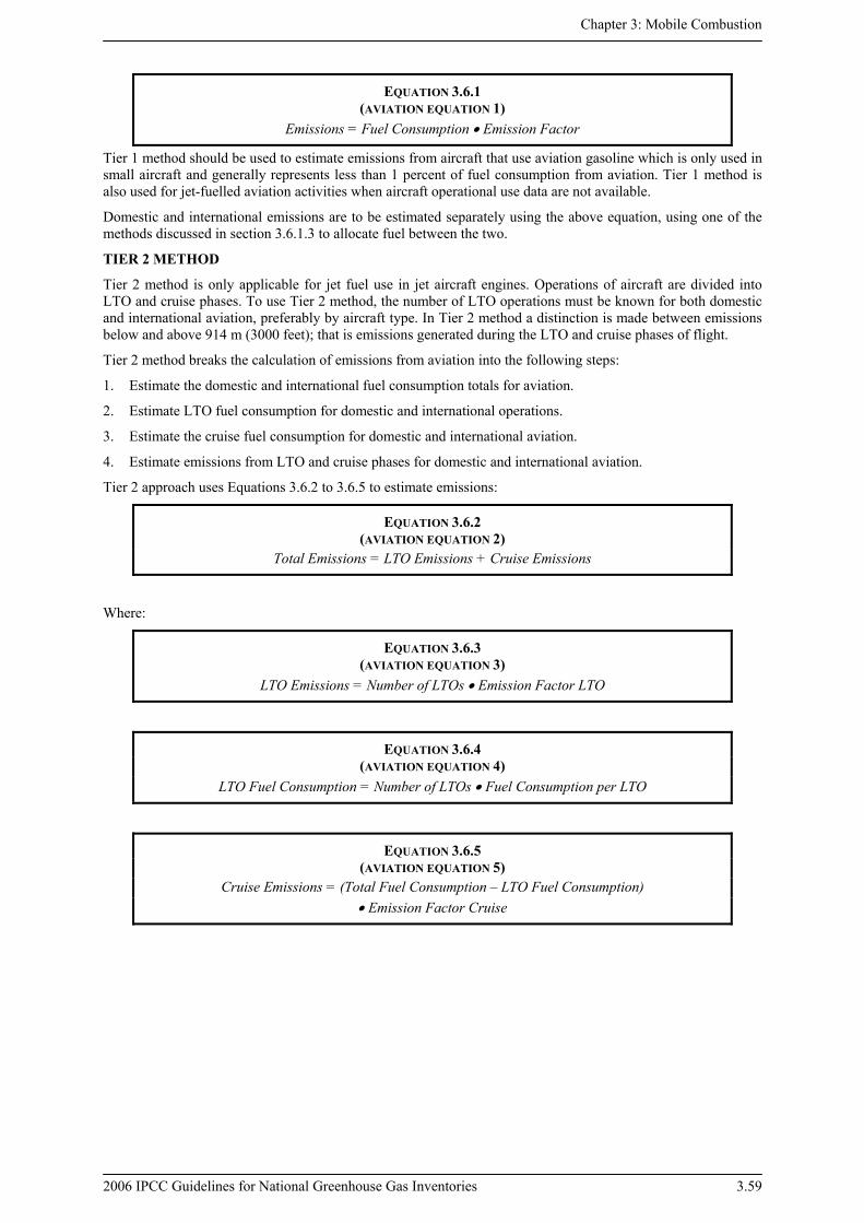
Chapter 3: Mobile Combustion
2006 IPCC Guidelines for National Greenhouse Gas Inventories 3.59
EQUATION 3.6.1 (AVIATION EQUATION 1)
Emissions = Fuel Consumption • Emission Factor
Tier 1 method should be used to estimate emissions from aircraft that use aviation gasoline which is only used in small aircraft and generally represents less than 1 percent of fuel consumption from aviation. Tier 1 method is also used for jet-fuelled aviation activities when aircraft operational use data are not available.
Domestic and international emissions are to be estimated separately using the above equation, using one of the methods discussed in section 3.6.1.3 to allocate fuel between the two.
TIER 2 METHOD
Tier 2 method is only applicable for jet fuel use in jet aircraft engines. Operations of aircraft are divided into LTO and cruise phases. To use Tier 2 method, the number of LTO operations must be known for both domestic and international aviation, preferably by aircraft type. In Tier 2 method a distinction is made between emissions below and above 914 m (3000 feet); that is emissions generated during the LTO and cruise phases of flight.
Tier 2 method breaks the calculation of emissions from aviation into the following steps:
1. Estimate the domestic and international fuel consumption totals for aviation.
2. Estimate LTO fuel consumption for domestic and international operations.
3. Estimate the cruise fuel consumption for domestic and international aviation.
4. Estimate emissions from LTO and cruise phases for domestic and international aviation.
Tier 2 approach uses Equations 3.6.2 to 3.6.5 to estimate emissions:
EQUATION 3.6.2 (AVIATION EQUATION 2)
Total Emissions = LTO Emissions + Cruise Emissions
Where:
EQUATION 3.6.3 (AVIATION EQUATION 3)
LTO Emissions = Number of LTOs • Emission Factor LTO
EQUATION 3.6.4 (AVIATION EQUATION 4)
LTO Fuel Consumption = Number of LTOs • Fuel Consumption per LTO
EQUATION 3.6.5 (AVIATION EQUATION 5)
Cruise Emissions = (Total Fuel Consumption – LTO Fuel Consumption) • Emission Factor Cruise
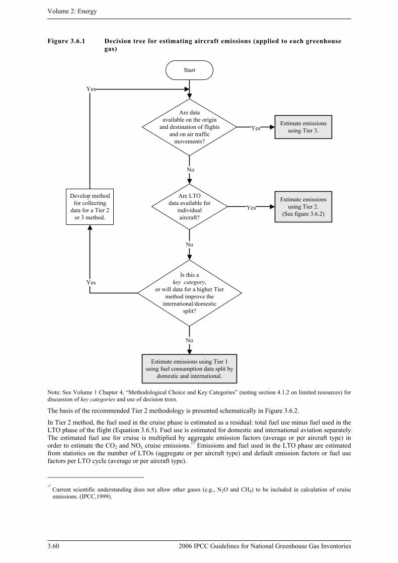
Volume 2: Energy
3.60 2006 IPCC Guidelines for National Greenhouse Gas Inventories
Figure 3.6.1 Decision tree for estimating aircraft emissions (applied to each greenhouse gas)
Start
Are dataavailable on the origin
and destination of flightsand on air traffic
movements?
Estimate emissionsusing Tier 3.Yes
No
Estimate emissions using Tier 1using fuel consumption data split by
domestic and international.
Are LTOdata available for
individualaircraft?
Yes
No
Is this akey category,
or will data for a higher Tier method improve the
international/domesticsplit?
No
Estimate emissionsusing Tier 2.
(See figure 3.6.2)
Develop method for collecting
data for a Tier 2or 3 method.
Yes
Yes
Note: See Volume 1 Chapter 4, “Methodological Choice and Key Categories” (noting section 4.1.2 on limited resources) for discussion of key categories and use of decision trees.
The basis of the recommended Tier 2 methodology is presented schematically in Figure 3.6.2.
In Tier 2 method, the fuel used in the cruise phase is estimated as a residual: total fuel use minus fuel used in the LTO phase of the flight (Equation 3.6.5). Fuel use is estimated for domestic and international aviation separately. The estimated fuel use for cruise is multiplied by aggregate emission factors (average or per aircraft type) in order to estimate the CO2 and NOx cruise emissions.17 Emissions and fuel used in the LTO phase are estimated from statistics on the number of LTOs (aggregate or per aircraft type) and default emission factors or fuel use factors per LTO cycle (average or per aircraft type).
17
Current scientific understanding does not allow other gases (e.g., N2O and CH4) to be included in calculation of cruise emissions. (IPCC,1999).

Chapter 3: Mobile Combustion
2006 IPCC Guidelines for National Greenhouse Gas Inventories 3.61
Tier 2 method considers activity data at the level of individual aircraft types and therefore needs data on the number of domestic LTOs by aircraft type and international LTOs by aircraft type. The estimate should include all aircraft types frequently used for domestic and international aviation. Table 3.6.3 provides a way of mapping actual aircraft to representative aircraft types in the database. Cruise emission factors for emissions other than NOx are not provided in Tier 2 method; either national emission factors or the tier default emission factors must be used to estimate these cruise emissions.
TIER 3 METHODS
Tier 3 methods are based on actual flight movement data, either: for Tier 3A origin and destination (OD) data or for Tier 3B full flight trajectory information. National Tier 3 approaches can be used if they are well documented and have been reviewed following the guidance provided in Volume 1, Chapter 6 (QA/QC). To facilitate data review, countries that use Tier 3 methodology could separately report emissions for Commercial Scheduled Aviation and Other Jet Fuelled Activities.
Tier 3A takes into account cruise emissions for different flight distances. Details on the origin (departure) and destination (arrival) airports and aircraft type are needed to use Tier 3A, for both domestic and international flights. In Tier 3A, inventories are modelled using average fuel consumption and emissions data for the LTO phase and various cruise phase lengths, for an array of representative aircraft categories.
The data used in Tier 3A methodology takes into account that the amount of emissions generated varies between phases of flight. The methodology also takes into account that fuel burn is related to flight distance, while recognizing that fuel burn can be comparably higher on relatively short distances than on longer routes. This is because aircraft use a higher amount of fuel per distance for the LTO cycle compared to the cruise phase.
The EMEP/CORINAIR Emission inventory guidebook (EEA 2002) provides an example of Tier 3A method for calculating emissions from aircraft. The EMEP/CORINAIR Emission inventory guidebook is continually being refined and is published electronically via the European Environment Agency Internet web site. EMEP/CORINAIR provides tables with emissions per flight distance.
(Note that there are three EMEP/CORINAIR methods for calculating aircraft emissions; but, only the Detailed CORINAIR Methodology equates to Tier 3A.)
Tier 3B methodology is distinguished from Tier 3A by the calculation of fuel burnt and emissions throughout the full trajectory of each flight segment using aircraft and engine-specific aerodynamic performance information. To use Tier 3B, sophisticated computer models are required to address all the equipment, performance and trajectory variables and calculations for all flights in a given year. Models used for Tier 3B level can generally specify output in terms of aircraft, engine, airport, region, and global totals, as well as by latitude, longitude, altitude and time, for fuel burn and emissions of CO, hydrocarbons (HC), CO2, H2O, NOx, and SOx. To be used in preparing annual inventory submissions, Tier 3B model must calculate aircraft emissions from input data that take into account air-traffic changes, aircraft equipment changes, or any input-variable scenario. The components of Tier 3B models ideally are incorporated so that they can be readily updated, so that the models are dynamic and can remain current with evolving data and methodologies. Examples of models include the System for assessing Aviation’s Global Emissions (SAGE), by the United States Federal Aviation Administration (Kim, 2005 a and b; Malwitz, 2005), and AERO2k, (Eyers, 2004), by the European Commission.
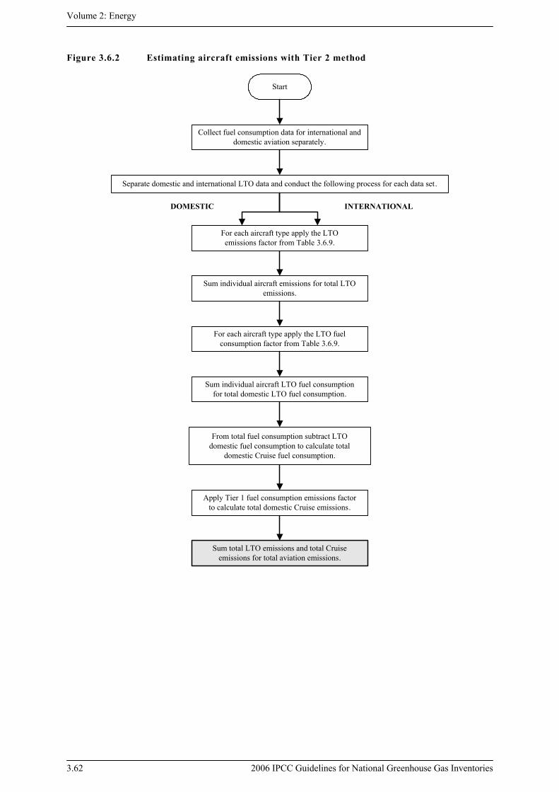
Volume 2: Energy
3.62 2006 IPCC Guidelines for National Greenhouse Gas Inventories
Figure 3.6.2 Estimating aircraft emissions with Tier 2 method
Start
Sum total LTO emissions and total Cruiseemissions for total aviation emissions.
Apply Tier 1 fuel consumption emissions factorto calculate total domestic Cruise emissions.
From total fuel consumption subtract LTOdomestic fuel consumption to calculate total
domestic Cruise fuel consumption.
Sum individual aircraft LTO fuel consumptionfor total domestic LTO fuel consumption.
For each aircraft type apply the LTO fuelconsumption factor from Table 3.6.9.
Sum individual aircraft emissions for total LTOemissions.
For each aircraft type apply the LTOemissions factor from Table 3.6.9.
Separate domestic and international LTO data and conduct the following process for each data set.
Collect fuel consumption data for international anddomestic aviation separately.
INTERNATIONALDOMESTIC
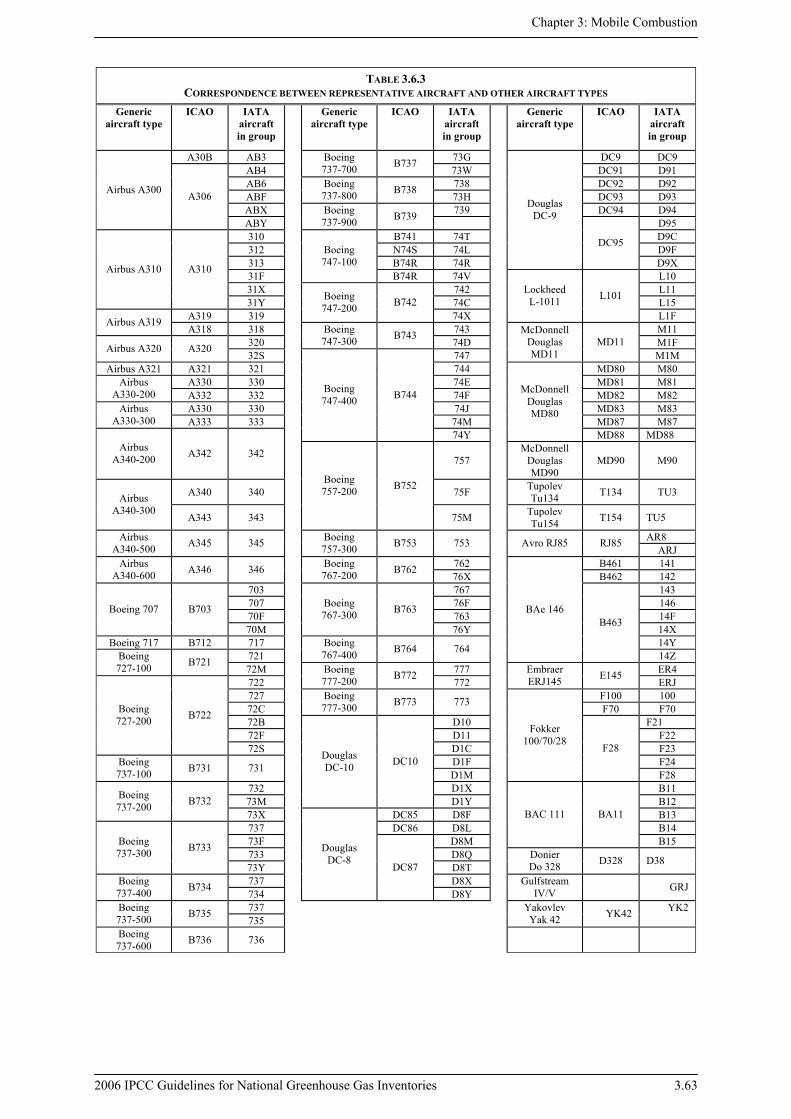
Chapter 3: Mobile Combustion
2006 IPCC Guidelines for National Greenhouse Gas Inventories 3.63
TABLE 3.6.3 CORRESPONDENCE BETWEEN REPRESENTATIVE AIRCRAFT AND OTHER AIRCRAFT TYPES
Generic aircraft type
ICAO IATA aircraft in group
Generic aircraft type
ICAO IATA aircraft in group
Generic aircraft type
ICAO IATA aircraft in group
A30B AB3 73G DC9 DC9 AB4
Boeing 737-700 B737
73W DC91 D91 AB6 738 DC92 D92 ABF
Boeing 737-800 B738
73H DC93 D93 ABX 739 DC94 D94
Airbus A300 A306
ABY Boeing 737-900 B739
D95 310 B741 74T D9C 312 N74S 74L D9F 313 B74R 74R
Douglas DC-9
DC95
D9X 31F
Boeing 747-100
B74R 74V L10 31X 742 L11
Airbus A310 A310
31Y 74C L15 A319 319
Boeing 747-200 B742
74X
Lockheed L-1011 L101
L1F Airbus A319 A318 318 743 M11
320 Boeing 747-300 B743
74D M1F Airbus A320 A320 32S 747
McDonnell Douglas MD11
MD11 M1M
Airbus A321 A321 321 744 MD80 M80 A330 330 74E MD81 M81 Airbus
A330-200 A332 332 74F MD82 M82 A330 330 74J MD83 M83 Airbus
A330-300 A333 333 74M MD87 M87
Boeing 747-400 B744
74Y
McDonnell Douglas MD80
MD88 MD88 Airbus
A340-200 A342 342 757
McDonnell Douglas MD90
MD90 M90
A340 340 75F Tupolev Tu134 T134 TU3 Airbus
A340-300 A343 343
Boeing 757-200 B752
75M Tupolev Tu154 T154 TU5
AR8 Airbus A340-500 A345 345 Boeing
757-300 B753 753 Avro RJ85 RJ85 ARJ
762 B461 141 Airbus A340-600 A346 346 Boeing
767-200 B762 76X B462 142
703 767 143 707 76F 146 70F 763 14F
Boeing 707 B703
70M
Boeing 767-300 B763
76Y 14X Boeing 717 B712 717 14Y
721 Boeing 767-400 B764 764
BAe 146 B463
14Z Boeing 727-100 B721
72M 777 ER4 722
Boeing 777-200 B772
772 Embraer ERJ145 E145
ERJ 727 F100 100 72C
Boeing 777-300 B773 773
F70 F70 72B D10 F21 72F D11 F22
Boeing 727-200 B722
72S D1C F23 D1F F24 Boeing
737-100 B731 731 D1M
Fokker 100/70/28
F28
F28 732 D1X B11 73M
Douglas DC-10 DC10
D1Y B12 Boeing 737-200 B732
73X DC85 D8F B13 737 DC86 D8L B14 73F D8M
BAC 111 BA11
B15 733 D8Q
Boeing 737-300 B733
73Y D8T Donier Do 328 D328 D38
737 D8X Boeing 737-400 B734
734
Douglas DC-8
DC87
D8Y Gulfstream
IV/V GRJ
737 Boeing 737-500 B735
735 Yakovlev
Yak 42 YK42 YK2
Boeing 737-600 B736 736

Volume 2: Energy
3.64 2006 IPCC Guidelines for National Greenhouse Gas Inventories
3.6.1.2 CHOICE OF EMISSION FACTORS
TIER 1
Carbon dioxide emission factors are based on the fuel type and carbon content. National emission factors for CO2 should not deviate much from the default values because the quality of jet fuel is well defined. It is good practice to use the default CO2 emission factors in Table 3.6.4 for Tier 1 (see Chapter 1, Introduction, of this Volume and Table 1.4). National carbon content could be used if available. CO2 should be estimated on the basis of the full carbon content of the fuel.
TABLE 3.6.4 CO2 EMISSION FACTORS
Fuel Default (kg/TJ) Lower Upper
Aviation Gasoline 70 000 67 500 73 000
Jet Kerosene 71 500 69 800 74 400
Default values for CH4 and N2O from aircraft are given in Table 3.6.5. Different types of aircraft/engine combinations have specific emission factors and these factors may also vary according to distance flown. Tier 1 assumes that all aircraft have the same emission factors for CH4 and N2O based on the rate of fuel consumption. This assumption has been made because more disaggregated emission factors are not available at this level of aggregation.
TABLE 3.6.5 NON-CO2 EMISSION FACTORS
Fuel
CH4 Default
(Uncontrolled) Factors (in kg/TJ)
N2O Default (Uncontrolled) Factors (in kg/TJ)
NOx Default (Uncontrolled) Factors (in kg/TJ)
All fuels 0.5a
(-57%/+100%)b2
(-70%/+150%) b250
+25% c a In the cruise mode CH4 emissions are assumed to be negligible (Wiesen et al., 1994). For LTO cycles only
(i.e., below an altitude of 914 metres (3000 ft.)) the emission factor is 5 kg/TJ (10% of total VOC factor) (Olivier, 1991). Since globally about 10% of the total fuel is consumed in LTO cycles (Olivier, 1995), the resulting fleet averaged factor is 0.5 kg/TJ. b IPCC, 1999. c Expert Judgement.
Emission factors for other gases (CO and NMVOC) and sulphur content which were included in the 1996 IPCC Guidelines can be found in the EFDB.
TIER 2
For Tier 2 method, it is good practice to use emission factors from Table 3.6.9 (or updates reflected in the EFDB) for the LTO emissions. For cruise calculations only NOx emissions can be computed directly based on specific emission factors (Table 3.6.10) and N2O can be computed indirectly from NOx emissions 18 . CO2 cruise emissions are calculated using Tier 1 CO2 emission factors (Table 3.6.4). The CH4 emissions are negligible and are assumed to be zero unless new information becomes available. Note that there is limited information on the emission factors for CH4 and N2O from aircraft, and the default values provided in Table 3.6.5 are similar to values found in the literature.
TIER 3
Tier 3A emission factors may be found in the EMEP/CORINAIR emission inventory guidebook, while Tier 3B uses emissions factors contained within the models necessary to employ this methodology. Inventory compilers should check that these emission factors are in fact appropriate.
18 Countries vary on the method to be used to convert NOx emissions to N2O

Chapter 3: Mobile Combustion
2006 IPCC Guidelines for National Greenhouse Gas Inventories 3.65
3.6.1.3 CHOICE OF ACTIVITY DATA Since emissions from domestic aviation are reported separately from international aviation, it is necessary to disaggregate activity data between domestic and international components. For this purpose, the following definitions should be applied irrespective of the nationality of the carrier (Table 3.6.6). For consistency, it is good practice to use similar definitions of domestic and international activities for aviation and water-borne navigation. In some cases, the national energy statistics may not provide data consistent with this definition. It is good practice that countries separate the activity data consistent with this definition. In any case, a country must clearly define the methodologies and assumptions used.
TABLE 3.6.6 CRITERIA FOR DEFINING INTERNATIONAL OR DOMESTIC AVIATION (APPLIES TO INDIVIDUAL LEGS OF
JOURNEYS WITH MORE THAN ONE TAKE-OFF AND LANDING)
Journey type between two airports Domestic International
Departs and arrives in same country Yes No
Departs from one country and arrives in another No Yes
Based on past experience compiling aviation emissions inventories, difficulties have been identified regarding the international/domestic split, in particular obtaining the information on passenger and freight drop-off and pick up at stops in the same country that was required by the 1996 IPCC Guidelines/GPG2000 (Summary report of ICAO/UNFCCC Expert Meeting April 2004). Most flight data are collected on the basis of individual flight segments (from one take-off to the next landing) and do not distinguish between different types of intermediate stops (as called for in GPG2000). Basing the distinction on flight segment data (origin/destination) is therefore simpler and is likely to reduce uncertainties. It is very unlikely that this change would make a significant change to the emission estimates.19 This does not change the way in which emissions from international flights are reported as a memo item and not included in national totals.
Improvements in technology and optimization of airline operating practices have significantly reduced the need for intermediate technical stops. An intermediate technical stop would also not change the definition of a flight as being domestic or international. For example if explicit data is available, countries may define as international flight segments that depart one country with a destination in another country and make an intermediate technical stop. A technical stop is solely for the purpose of refuelling or solving a technical difficulty and not for the purpose of passenger or cargo exchange.
If national energy statistics do not already provide data consistent with this definition, countries should then estimate the split between domestic and international fuel consumption according to the definition, using the approaches set out below.
Top-down data can be obtained from taxation authorities in cases where fuel sold for domestic use is subject to taxation, but that for international use is not taxed. Airports or fuel suppliers may have data on delivery of aviation kerosene and aviation gasoline to domestic and to international flights. In most countries tax and custom dues are levied on fuels for domestic consumption, and fuels for international consumption (bunkers) are free of such dues. In the absence of more direct sources of data, information about domestic taxes may be used to distinguish between domestic and international fuel consumption.
Bottom-up data can be obtained from surveys of airline companies for fuel used on domestic and international flights, or estimates from aircraft movement data and standard tables of fuel consumed or both. Fuel consumption factors for aircraft (fuel used per LTO and per nautical mile cruised) can be used for estimates and may be obtained from the airline companies.
Examples of sources for bottom-up data, including aircraft movement, are:
• Statistical offices or transport ministries as a part of national statistics;
• Airport records;
• ATC (Air Traffic Control) records, for example EUROCONTROL statistics;
19 It is good practice to clearly state the reasoning and justification if any country opts to use the GPG2000 definitions.
Volume 2: Energy
3.66 2006 IPCC Guidelines for National Greenhouse Gas Inventories
• Air carrier schedules published monthly by OAG which contains worldwide timetable passenger and freight aircraft movements as well as regular scheduled departures of charter operators. It does not contain ad-hoc charter aircraft movements;
Some of these sources do not cover all flights (e.g. charter flights may be excluded). On the other hand, airline timetable data may include duplicate flights due to codeshares between airlines or duplicate flight numbers. Methods have been developed to detect and remove these duplicates. (Baughcum et al., 1996; Sutkus et al., 2001).
The aircraft types listed in Table 3.6.9, LTO Emission Factors were defined based on the assumptions listed below. Aircraft were divided into four major groups to reflect and note the distinct data source for each group:
Large Commercial Aircraft: This includes aircraft that reflect the 2004 operating fleet and some aircraft types for back compatibility, identified by minor model. It was felt that this method would most accurately reflect operational fleet emissions. To minimize table size, some aircraft minor models were grouped when LTO emissions factors were similar. The Large Commercial Aircraft group LTO emissions factors data source is the ICAO Engine Exhaust Emissions Data Bank (ICAO, 2004a).
Regional Jets: This group includes aircraft that are representative of the 2004 operating Regional Jet (RJ) fleet. Representative RJ aircraft were selected based on providing an appropriate range of RJ aircraft with LTO emissions factors available. The RJ group LTO emissions factors data source is the ICAO Engine Exhaust Emissions Data Bank (ICAO, 2004a).
Low Thrust Jets: In some countries, aircraft in the low thrust category (engines with thrust below 26.7 kN) make up a non-trivial number of movements and therefore should be included in inventories. However, aircraft engines in this group are not required to satisfy ICAO engine emissions standards, thus LTO emissions factors data are not included in the ICAO Engine Exhaust Emissions Data Bank and difficult to provide. Therefore, there is one representative aircraft with typical emissions for aircraft in this group. The Low Thrust Jets group LTO emissions factors data source is the FAA’s Emissions and Dispersion Modelling System (EDMS) (FAA 2004b).
Turboprops: This group includes aircraft that are representative of the 2004 Turboprop fleet, which can be represented by three typical aircraft size based on engine shaft horsepower. The Turboprop group LTO emissions factors data source is the Swedish Aeronautical Institute (FOI) LTO Emissions Database. Similar data could be obtained from other sources (e.g. EEA, 2002). The equivalent data for turboprop and piston engine aircraft need to be obtained from other sources. The relationship between actual aircraft and representative aircraft are provided in the Table 3.6.3.
Aircraft Fleet data may be obtained from various sources. ICAO collects fleet data through two of its statistics sub-programmes: the fleet of commercial air carriers, reported by States for their commercial air carriers, and civil aircraft on register, reported by States for the civil aircraft on their register at 31 December (ICAO 2004b).
Some ICAO States do not participate in this data collection, in part because of the difficulty to split the fleet into commercial and non-commercial entities. Because of this, ICAO also makes use of other external sources. One of these sources is the International Register of Civil Aircraft, 2004, published by the Bureau Veritas (France), the CAA (UK) and ENAC (Italy) in cooperation with ICAO. This database contains the information from the civil aircraft registers of some 45 States (including the United States) covering over 450 000 aircraft.
In addition to the above, there are commercial databases of which ICAO also makes use. None of them cover the whole fleet as they have limitations in scope and aircraft size. Among these one can find the BACK Aviation Solutions Fleet Data (fixed wing aircraft over 30 seats), AirClaims CASE database (fixed wing jet and turboprop commercial aircraft), BUCHAir, publishers of the JP Airline Fleet (covers both fixed and rotary wing aircraft). Other companies such as AvSoft may also have relevant information. Further information may be obtained from these companies’ websites.
3.6.1.4 MILITARY AVIATION Military activity is defined here as those activities using fuel purchased by or supplied to the military authorities of the country. Emissions from aviation fuel use can be estimated using equation 3.6.1 and the same calculations approach recommended for civilian aviation. Some types of military transport aircraft and helicopters have fuel and emissions characteristics similar to civil types. Therefore default emission factors for civil aircraft should be used for military aviation unless better data are available. Alternatively, fuel use may be estimated from the hours in operation. Default fuel consumption factors for military aircraft are given in Tables 3.6.7 and 3.6.8. For fuel use factors see Section 3.6.1.3 ‘Choice of activity data’.

Chapter 3: Mobile Combustion
2006 IPCC Guidelines for National Greenhouse Gas Inventories 3.67
TABLE 3.6.7 FUEL CONSUMPTION FACTORS FOR MILITARY AIRCRAFT
Group Sub- group Representative type Fuel flow(kg/hour)
Combat Fast Jet – High Thrust Fast Jet – Low Thrust
F16 Tiger F-5E
3 283
2 100
Trainer Jet trainers Turboprop trainers
Hawk PC-7
720
120
Tanker/transport Large tanker/ transport
Small Transport
C-130 ATP
2 225
499
Other MPAs Maritime Patrol C-130 2 225
Sources: Tables 3.1 and 3.2 of Gardner et. al 1998 USEPA, 2005)
TABLE 3.6.8 FUEL CONSUMPTION PER FLIGHT HOUR FOR MILITARY AIRCRAFT
AIRCRAFT TYPE Aircraft Description
FUEL USE (LITRES PER
HOUR)
A-10A Twin engine light bomber 2 331
B-1B Four engine long-range strategic bomber. Used by USA only 13 959
B-52H Eight engine long-range strategic bomber. Used by USA only. 12 833
C-12J Twin turboprop light transport. Beech King Air variant. 398
C-130E Four turboprop transport. Used by many countries. 2 956
C-141B Four engine long-range transport. Used by USA only 7 849
C-5B Four engine long-range heavy transport. Used by USA only 13 473
C-9C Twin engine transport. Military variant of DC-9. 3 745
E-4B Four engine transport. Military variant of Boeing 747. 17 339
F-15D Twin engine fighter. 5 825
F-15E Twin engine fighter-bomber 6 951
F-16C Single engine fighter. Used by many countries. 3 252
KC-10A Three engine tanker. Military variant of DC-10 10 002
KC-135E Four engine tanker. Military variant of Boeing 707. 7 134
KC-135R Four engine tanker with newer engines. Boeing 707 variant. 6 064
T-37B Twin engine jet trainer. 694
T-38A Twin engine jet trainer. Similar to F-5. 262
Military aircraft (transport planes, helicopters and fighters) may not have a civilian analogue, so a more detailed method of data analysis is encouraged where data are available. Inventory compilers should consult military experts to determine the most appropriate emission factors for the country’s military aviation.
Due to confidentiality issues (see completeness and reporting), many inventory compilers may have difficulty obtaining data for the quantity of fuel used by the military. Military activity is defined here as those activities using fuel purchased by or supplied to the military authorities in the country. Countries can apply the rules defining civilian, national and international aviation operations to military operations when the data necessary to apply those rules are comparable and available. In this case, the international military emissions may be reported under International Aviation (International Bunkers), but must then be shown separately. Data on military fuel

Volume 2: Energy
3.68 2006 IPCC Guidelines for National Greenhouse Gas Inventories
use should be obtained from government military institutions or fuel suppliers. If data on fuel split are unavailable, all the fuel sold for military activities should be treated as domestic.
Emissions resulting from multilateral operations pursuant to the Charter of the United Nations should not be included in national totals; other emissions related to operations shall be included in the national emissions totals of one or more Parties involved. The national calculations should take into account fuel delivered to the country’s military, as well as fuel delivered within that country but used by the military of other countries. Other emissions related to operations (e.g., off-road ground support equipment) shall be included in the national emissions totals in the appropriate source category.
These data should be used with care as national circumstances may vary from those assumed in this table. In particular, distances travelled and fuel consumption may be affected by national route structures, airport congestion and air traffic control practices.
3.6.1.5 COMPLETENESS Regardless of method, it is important to account for all fuel used for aviation in the country. The methods are based on total fuel use, and should completely cover CO2 emissions. However, the allocation between LTO and cruise will not be complete for Tier 2 method if the LTO statistics are not complete. Also, Tier 2 method focuses on passenger and freight carrying scheduled and charter flights, and thus not all aviation. In addition, Tier 2 method does not automatically include non-scheduled flights and general aviation such as agricultural airplanes, private jets or helicopters, which should be added if the quantity of fuel is significant. Completeness may also be an issue where military data are confidential; in this situation it is good practice to aggregate military fuel use with another source category.
Other aviation-related activities that generate emissions include: fuelling and fuel handling in general, maintenance of aircraft engines and fuel jettisoning to avoid accidents. Also, in the wintertime, anti-ice and de-ice treatment of wings and aircraft is a source of emissions at airport complexes. Many of the materials used in these treatments flow off the wings when planes are idling, taxiing, and taking off, and then evaporate. These emissions are, however, very minor and specific methods to estimate them are not included.
There are additional challenges in distinguishing between domestic and international emissions. As each country’s data sources are unique for this category, it is not possible to formulate a general rule regarding how to make an assignment in the absence of clear data. It is good practice to specify clearly the assumptions made so that the issue of completeness can be evaluated.
3.6.1.6 DEVELOPING A CONSISTENT TIME SERIES Volume 1 Chapter 5: Time Series Consistency and Recalculation of the 2006 IPCC Guidelines provides more information on how to develop emission estimates in cases where the same data sets or methods cannot be used during every year of the time series. If activity data are unavailable for the base year (e.g. 1990) an option may be to extrapolate data to this year by using changes in freight and passenger kilometres, total fuel used or supplied, or the number of LTOs (aircraft movements).
Emissions trends of CH4 and NOx (and by inference N2O) will depend on aircraft engine technology and the change in composition of a country's fleet. This change in fleet composition may have to be accounted for in the future, and this is best accomplished using Tier 2 and Tier 3B methods based on individual aircraft types for 1990 and subsequent years. If fleet composition is not changing, the same set of emission factors should be used for all years.
Every method should be able to reflect accurately the results of mitigation options that lead to changes in fuel use. However, only Tier 2 and 3B methods, based on individual aircraft, can capture the effect of mitigation options that result in lower emission factors.
Tier 2 has been revised to account for NOx emissions in the climb phase, which are substantially different from those in cruise, and the differences in the amount of NOx calculated during that phase could be in the range of approximately 15 to 20 percent, due to the thrust/power required in that phase, and its relation with the higher production of NOx. Special care should be taken to develop a consistent time series if Tier 2 is used.

Chapter 3: Mobile Combustion
2006 IPCC Guidelines for National Greenhouse Gas Inventories 3.69
3.6.1.7 UNCERTAINTY ASSESSMENT
EMISSION FACTORS
The CO2 emission factors should be within a range of ±5 percent, as they are dependent only on the carbon content of the fuel and fraction oxidised. However, considerable uncertainty is inherent in the computation of CO2 based on the uncertainties in activity data discussed below. For Tier 1, the uncertainty of the CH4 emission factor may range between -57 and +100 percent. The uncertainty of the N2O emission factor may range between -70 and +150 percent Moreover, CH4 and N2O emission factors vary with technology and using a single emission factor for aviation in general is a considerable simplification.
Information to assist in computing uncertainties associated with LTO emission factors found in Table 3.6.9 can be found in Lister and Norman, 2003; and ICAO, 1993. Information to assist in computing the uncertainties associated with cruise emission factors found in Table 3.6.10 data can be found in: Baughcum et al, 1996. Sutkus, et al, 2001; Eyers et al, 2004; Kim, 2005 a and b; Malwitz, 2005. If resources are not available to compute uncertainties, uncertainty bands can be used as defined as default factors in Section 3.6.1.2.
Special attention should be taken with the cruise NOx emission factors for Tier 2 found in Table 3.6.10. These emission factors, have been updated from the 1996 Guidelines to reflect the fact that climb phase emissions are substantially different from those in cruise. The calculation of the NOx emission factors is based on two sets of data, one from 1 km to 9 km, and the second from 9 km to 13 km., and the differences in the amount of NOx calculated during that phase could be in the range of approximately 15 to 20 percent, due to the thrust/power required in that phase, and its relation with the higher production of NOx. If Tier 2 is used, care should be taken to report a consistent time series (see Section 3.6.1.6 and Volume 1, Chapter 5).
ACTIVITY DATA
The uncertainty in the reporting will be strongly influenced by the accuracy of the data collected on domestic aviation separately from international aviation. With complete survey data, the uncertainty may be very low (less than 5 percent) while for estimates or incomplete surveys the uncertainties may become large, perhaps a factor of two for the domestic share. The uncertainty ranges cited represent an informal polling of experts aiming to approximate the 95 percent confidence interval around the central estimate. The uncertainty will vary widely from country to country and is difficult to generalise. The use of global data sets, supported by radar, may be helpful in this area, and it is expected that reporting will improve for this category in the future.
3.6.2 Inventory Quality Assurance/Quality Control (QA/QC)
It is good practice to conduct quality control checks as outlined in Chapter 6 of Volume 1 (Quality Assurance/ Quality Control and Verification), Tier 1 General Inventory Level QC Procedures. It is good practice to conduct expert review of the emission estimates when using Tier 2 or 3 methods. Additional quality control checks as outlined in Tier 2 procedures in the same chapter and quality assurance procedures may also be applicable, particularly if higher tier methods are used to determine emissions from this source category. Inventory compilers are encouraged to use higher tier QA/QC for key categories as identified in Chapter 4 of Volume I.
Specific procedures relevant to this source category are outlined below.
Comparison of emissions using alternative approaches
If higher tier approaches are used, the inventory compiler should compare inventories to estimates with lower tiers. Any anomaly between the emission estimates should be investigated and explained. The results of such comparisons should be recorded for internal documentation.
Review of Emission factors
If national factors are used rather than the default values, directly reference the QC review associated with the publication of the emission factors, and include this review in the QA/QC documentation to ensure that the procedures are consistent with good practice. If possible, the inventory compiler should compare the IPCC default values to national factors to provide further indication that the factors are applicable. If emissions from military use were developed using data other than the default factors, the accuracy of the calculations and the applicability and relevance of the data should be checked.

Volume 2: Energy
3.70 2006 IPCC Guidelines for National Greenhouse Gas Inventories
TABLE 3.6.9 LTO EMISSION FACTORS FOR TYPICAL AIRCRAFT
LTO emissions factors (kg/LTO/) (12)
AIRCRAFT CO2
(11) CH4(7) N2O(9) NOX CO NMVOC(8) SO2
(10)
LTO FUEL CONSUMPTION
(Kg/LTO)
A300 5450 0.12 0.2 25.86 14.80 1.12 1.72 1720
A310 4760 0.63 0.2 19.46 28.30 5.67 1.51 1510
A319 2310 0.06 0.1 8.73 6.35 0.54 0.73 730
A320 2440 0.06 0.1 9.01 6.19 0.51 0.77 770
A321 3020 0.14 0.1 16.72 7.55 1.27 0.96 960
A330-200/300 7050 0.13 0.2 35.57 16.20 1.15 2.23 2230
A340-200 5890 0.42 0.2 28.31 26.19 3.78 1.86 1860
A340-300 6380 0.39 0.2 34.81 25.23 3.51 2.02 2020
A340-500/600 10660 0.01 0.3 64.45 15.31 0.13 3.37 3370
707 5890 9.75 0.2 10.96 92.37 87.71 1.86 1860
717 2140 0.01 0.1 6.68 6.78 0.05 0.68 680
727-100 3970 0.69 0.1 9.23 24.44 6.25 1.26 1260
727-200 4610 0.81 0.1 11.97 27.16 7.32 1.46 1460
737-100/200 2740 0.45 0.1 6.74 16.04 4.06 0.87 870
737-300/400/500 2480 0.08 0.1 7.19 13.03 0.75 0.78 780
737-600 2280 0.10 0.1 7.66 8.65 0.91 0.72 720
737-700 2460 0.09 0.1 9.12 8.00 0.78 0.78 780
737-800/900 2780 0.07 0.1 12.30 7.07 0.65 0.88 880
747-100 10140 4.84 0.3 49.17 114.59 43.59 3.21 3210
747-200 11370 1.82 0.4 49.52 79.78 16.41 3.60 3600
747-300 11080 0.27 0.4 65.00 17.84 2.46 3.51 3510
747-400 10240 0.22 0.3 42.88 26.72 2.02 3.24 3240
757-200 4320 0.02 0.1 23.43 8.08 0.20 1.37 1370
757-300 4630 0.01 0.1 17.85 11.62 0.10 1.46 1460
767-200 4620 0.33 0.1 23.76 14.80 2.99 1.46 1460
767-300 5610 0.12 0.2 28.19 14.47 1.07 1.77 1780
767-400 5520 0.10 0.2 24.80 12.37 0.88 1.75 1750
777-200/300 8100 0.07 0.3 52.81 12.76 0.59 2.56 2560
DC-10 7290 0.24 0.2 35.65 20.59 2.13 2.31 2310
DC-8-50/60/70 5360 0.15 0.2 15.62 26.31 1.36 1.70 1700
DC-9 2650 0.46 0.1 6.16 16.29 4.17 0.84 840
Larg
e C
omm
erci
al A
ircra
ft (1
) (2)
L-1011 7300 7.40 0.2 31.64 103.33 66.56 2.31 2310

Chapter 3: Mobile Combustion
2006 IPCC Guidelines for National Greenhouse Gas Inventories 3.71
TABLE 3.6.9 (CONTINUED)
LTO EMISSION FACTORS FOR TYPICAL AIRCRAFT
LTO emissions factors (kg/LTO/) (12)
AIRCRAFT CO2
(11) CH4(7) N2O(9) NOX CO NMVOC(8) SO2
(10)
LTO FUEL CONSUMPTION
(KG/LTO)
MD-11 7290 0.24 0.2 35.65 20.59 2.13 2.31 2310
MD-80 3180 0.19 0.1 11.97 6.46 1.69 1.01 1010
MD-90 2760 0.01 0.1 10.76 5.53 0.06 0.87 870
TU-134 2930 1.80 0.1 8.68 27.98 16.19 0.93 930
TU-154-M 5960 1.32 0.2 12.00 82.88 11.85 1.89 1890
TU-154-B 7030 11.90 0.2 14.33 143.05 107.13 2.22 2230
RJ-RJ85 1910 0.13 0.1 4.34 11.21 1.21 0.60 600
BAE 146 1800 0.14 0.1 4.07 11.18 1.27 0.57 570
CRJ-100ER 1060 0.06 0.03 2.27 6.70 0.56 0.33 330
ERJ-145 990 0.06 0.03 2.69 6.18 0.50 0.31 310
Fokker 100/70/28 2390 0.14 0.1 5.75 13.84 1.29 0.76 760
BAC111 2520 0.15 0.1 7.40 13.07 1.36 0.80 800
Dornier 328 Jet 870 0.06 0.03 2.99 5.35 0.52 0.27 280
Gulfstream IV 2160 0.14 0.1 5.63 8.88 1.23 0.68 680
Gulfstream V 1890 0.03 0.1 5.58 8.42 0.28 0.60 600
Reg
iona
l Jet
s
Yak-42M 2880 0.25 0.1 10.66 10.22 2.27 0.91 910
Jets
(3
) (F
n Cessna 525/560 1070 0.33 0.03 0.74 34.07 3.01 0.34 340
Beech King Air (5) 230 0.06 0.01 0.30 2.97 0.58 0.07 70
DHC8-100 (6) 640 0.00 0.02 1.51 2.24 0.00 0.20 200
Turb
opro
ps4)
ATR72-500 (7) 620 0.03 0.02 1.82 2.33 0.26 0.20 200
Notes: (1) ICAO Engine Exhaust Emissions Data Bank (ICAO, 2004) based on average measured data. Emissions factors apply to LTO
(Landing and Take off) only. (2) Engine types for each aircraft were selected on a consistent basis of the engine with the most LTOs. This approach, for some engine
types, may underestimate (or overestimate) fleet emissions which are not directly related to fuel consumption (eg NOx, CO, HC). (2) Emissions and Dispersion Modelling System (EDMS) (FAA 2004b) (4) FOI (The Swedish Defence Research Agency) Turboprop LTO Emissions database (5) Representative of Turboprop aircraft with shaft horsepower of up to 1000 shp/engine (6) Representative of Turboprop aircraft with shaft horsepower of 1000 to 2000 shp/engine (7) Representative of Turboprop aircraft with shaft horsepower of more than 2000 shp/engine (8) Assuming 10% of total VOC emissions in LTO cycles are methane emissions (Olivier, 1991) (as in the 1996 IPCC Guidelines). (9) Estimates based on Tier I default values (EF ID 11053) (as in the 1996 IPCC Guidelines). (10) The sulphur content of the fuel is assumed to be 0.05% (as in the 1996 IPCC Guidelines). (11) CO2 for each aircraft based on 3.16 kg CO2 produced for each kg fuel used, then rounded to the nearest 10 kg. (12) Information regarding the uncertainties associated with this data can be found in: Lister and Norman, 2003; ICAO, 1993. Table prepared in 2005 updates will be available in the Emission Factor Data Base.

Volume 2: Energy
3.72 2006 IPCC Guidelines for National Greenhouse Gas Inventories
TABLE 3.6.10 NOX EMISSION FACTORS FOR VARIOUS AIRCRAFT AT CRUISE LEVELS
Aircraft NOx Emission Factor (g/kg) (1) (5) A300 14.8 A310 12.2 A319 11.6 A320 12.9 A321 16.1
A330-200/300 13.8 A340-200 14.5 A340-300 14.6
A340-500/600 13.0 (2) 707 5.9 717 11.5 (3)
727-100 8.7 727-200 9.5
737-100/200 8.7 737-300/400/500 11.0
737-600 12.8 737-700 12.4
737-800/900 14.0 747-100 15.5 747-200 12.8 747-300 15.2 747-400 12.4 757-200 11.8 757-300 9.8 (3) 767-200 13.3 767-300 14.3 767-400 13.7 (3)
777-200/300 14.1 DC-10 13.9
DC-8-50/60/70 10.8 DC-9 9.1
L-1011 15.7 MD-11 13.2 MD-80 12.4 MD-90 14.2 TU-134 8.5
TU-154-M 9.1
Larg
e C
omm
erci
al A
ircra
ft
TU-154-B 9.1 RJ-RJ85 15.6 BAE 146 8.4
CRJ-100ER 8.0 ERJ-145 7.9
Fokker 100/70/28 8.4 BAC111 12.0
Dornier 328 Jet 14.8 (2) Gulfstream IV 8.0 (2) Gulfstream V 9.5 (2)
Reg
iona
l Jet
s
Yak-42M 15.6 (4)
Low
Th
rust
Je
ts (F
n <
26.7
kN
)
Cessna 525/560 7.2 (4)
Beech King Air 8.5 DHC8-100 12.8
Turb
opro
ps
ATR72-500 14.2
Notes: (1) Sutkus et al 2001, Unless otherwise noted. (2) Data from SAGE model Kim, 2005 a and b; Malwitz, 2005 (3) Sutkus, Baughcum, DuBois, 2003 (4) Average of the data from SAGE (Kim, 2005 a and b; Malwitz, 2005) and AERO2k (Eyers et al, 2004) (5) Information to assist in computing uncertainties can be found in: Baughcum et al, 1996; Sutkus, et al, 2001; Eyers et al, 2004; Kim, 2005 a and b; Malwitz, 2005.

Chapter 3: Mobile Combustion
2006 IPCC Guidelines for National Greenhouse Gas Inventories 3.73
Activity data check
The source of the activity data should be reviewed to ensure applicability and relevance to the source category. Where possible, the inventory compiler should compare current data to historical activity data or model outputs to look for anomalies. In preparing the inventory estimates, the inventory compiler should ensure the reliability of the activity data used to differentiate emissions between domestic and international aviation.
Data can be checked with productivity indicators such as fuel per unit of traffic performance (per passenger km or ton km). Where data from different countries are being compared, the band of data should be small. The European Environmental Agency provides a useful dataset20 which presents emissions and passenger/freight volume for each transportation mode for Europe. For example, Norway estimates that for domestic aviation, emissions are 0.22 kg CO2/passenger-km. However, note that the global fleet includes many small aircraft with relatively low energy efficiency. The U.S. Department of Transportation estimates an average energy intensity for the U.S. fleet of 3666 Btu/passenger mile (2403 kJ/passenger km). The International Air Transport Association estimates that the average aircraft consumes 3.5 litres of jet fuel per 100 passenger-km (67 passenger miles per U.S. gallon).
Reliance on scheduled operations for activity data may introduce higher uncertainties than simple reliance on fuel use for CO2. However, fuel loss and use of jet fuel for other activities will result in over estimates of aviation’s contributions.
External review
The inventory compiler should perform an independent, objective review of calculations, assumptions or documentation of the emissions inventory to assess the effectiveness of the QC programme. The review should be performed by expert(s) (e.g. aviation authorities, airline companies, and military staff) who are familiar with the source category and who understand inventory requirements.
3.6.3 Reporting and Documentation It is good practice to document and archive all information required to produce the national emissions inventory estimates as outlined in Chapter 8 of Volume 1 of the 2006 IPCC Guidelines. Some examples of specific documentation and reporting relevant to this source category are provided below.
Inventory compilers are required to report emissions from international aviation separately from domestic aviation, and exclude international aviation from national totals. It is expected that all countries have aviation activity and should therefore report emissions from this category. Though countries covering small areas might not have domestic aviation, emissions from international aviation should be reported. Inventory compilers should explain how the definition for international and domestic in the guidelines has been applied.
Transparency would be improved if inventory compilers provide data on emissions from LTO separately from cruise operations. Emissions from military aviation should be clearly specified, so as to improve the transparency on national greenhouse gas inventories. In addition to the numerical information reported in the standard tables, provision of the following data would increase transparency:
• Sources of fuel data and other essential data (e.g. fuel consumption factors) depending on the method used;
• The number of flight movements split between domestic and international;
• Emission factors used, if different from default values. Data sources should be referenced.
• If Tier 3 method is used, emissions data could be provided separately for Commercial Scheduled Aviation and Other Jet Fuelled Activities.
Confidentiality may be a problem if only one or two airline companies operate domestic transport in a given country. Confidentiality may also be a problem for reporting military aviation in a transparent manner.
3.6.4 Reporting tables and worksheets The four pages of the worksheets (Annex 1) for the Tier 1 Sectoral Approach are to be filled in for each of the source categories in Table 3.6.1. The reporting tables are available in Volume 1, Chapter 8.
20 See http://air-climate.eionet.eu.int/databases/TRENDS/TRENDS_EU15_data_Sep03.xls

Volume 2: Energy
3.74 2006 IPCC Guidelines for National Greenhouse Gas Inventories
3.6.5 Definitions of specialist terms Aviation Gasoline - A fuel used only in small piston engine aircraft, and which generally represents less than 1% of fuel used in aviation
Climb – The part of a flight of an aircraft, after take off and above 914 meters (3000 feet) above ground level, consisting of getting an aircraft to the desired cruising altitude.
Commercial scheduled – All commercial aircraft operations that have publicly available schedules (e.g., the Official Airline Guide, OAG 2006), which would primarily include passenger services. Activities that do not operate with publicly available schedules are not included in this definition, such as non-scheduled cargo, charter, air-taxi and emergency response operations. Note: Commercial Scheduled Aviation is used as a subset of jet fuel powered aviation operations.
Cruise – All aircraft activities that take place at altitudes above 914 meters (3000 feet), including any additional climb or descent operations above this altitude. No upper limit is given.
Gas Turbine Engines – Rotary engines that extract energy from a flow of combustion gas. Energy is added to the gas stream in the combustor, where air is mixed with fuel and ignited. Combustion increases the temperature and volume of the gas flow. This is directed through a nozzle over a turbine's blades, spinning the turbine and powering a compressor. For an aircraft, energy is extracted either in the form of thrust or through a turbine driving a fan or propeller.
References ROAD TRANSPORTATION ADEME/DIREM (2002). Agence de l’Environnement et de la Maltrlse de l’Energle, La direction des ressources
énergétiques et minérales, Ecobilan, PricewaterhouseCoopers, ‘Energy and greenhouse gas balances of biofuels’ production chains in France.’ December, www.ademe.fr/partenaires/agrice/publications/ ocuments_anglais/synthesis_energy_and_greenhouse_english.pdf
ARB (2004). ‘Technical Support Document for Staff Proposal Regarding Reduction of greenhouse gas emissions from motor vehicles, climate change emissions inventory’. California Air Resources Board (August 6 2004)
Ballantyne, V. F., Howes, P., and Stephanson, L. (1994). ‘Nitrous oxide emissions from light duty vehicles.’ SAE Tech. Paper Series (#940304), 67–75.
Beer, T., Grant, T., Brown, R., Edwards, J., Nelson, P., Watson, H., Williams, D., (2000). ‘Life-cycle emissions analysis of alternative fuels for heavy vehicles’. CSIRO Atmospheric Research Report C/0411/1.1/F2 to the Australian Greenhouse Office, Australia. (March 2000)
Behrentz, E. (2003). ‘Measurements of nitrous oxide emissions from light-duty motor vehicles: analysis of important variables and implications for California´s greenhouse gas emission Inventory.’ Dissertation Prospectus University of California, USA, (2003). See http://ebehrent.bol.ucla.edu/N2O.pdf
Borsari, V. (2005). ‘As emissoes veiculares e os gases de efeito estufa.’ SAE - Brazilian Society of Automotive Engineers
CETESB (2004). Air Quality Report (Relatório de Qualidade do Ar 2003, in Portuguese, (Air Quality Report 2003), available at http://www.cetesb.sp.gov.br/Ar/Relatorios/RelatorioAr2003.zip and
CETESB (2005). Personal communication with Oswaldo Lucon, São Paulo State Environment Agency, Mobile Sources Division. Information based on measurements conducted by Renato Linke, Vanderlei Borsari and Marcelo Bales, (Vehicle Inspection Division, ph. +5511 3030 6000). Partially published.
CONCAWE Report 2/02 Brussels, Belgium, (April 2002). ‘Energy and greenhouse gas balance of biofuels for Europe - an update.’
Díaz, L. et.al (2001). ‘Long-term efficiency of catalytic converters operating in Mexico City.’ Air & Waste Management Association, ISSN 1047-3289, Vol 51, pp.725-732,

Chapter 3: Mobile Combustion
2006 IPCC Guidelines for National Greenhouse Gas Inventories 3.75
EEA (2000). European Environment Agency (EEA). ‘COPERT III computer programe to calculate emissions from road transport, methodology and emission factors report.’ (Version 2.1), Copenhagen, Denmark November 2000. (For more details see http://vergina.eng.auth.gr/mech/lat/copert/copert.htm)
EEA (2005a). EMEP/CORINAIR. Emission Inventory Guidebook – 2005 European Environment Agency, Technical report No 30. Copenhagen, Denmark, (December 2005). Available from web site: http://reports.eea.eu.int/EMEPCORINAIR4/en
EEA (2005b). European Environment Agency (EEA), Computer programme to calculate emissions from road transport (COPERT), http:/vergina.eng.auth.gr/mech/lat/copert/copert.htm
Gamas, D.J., Diaz, L., Rodriguez, R., López-Salinas, E., Schifter, I.,. (1999). ‘Exhaust emissions from gasoline and LPG-powered vehicles operating at the altitude of Mexico City.’ in Journal of the Air & Waste Management Association, October 1999.
Heeb, Norbert., et al (2003). ‘Methane, benzene and alkyl benzene cold start emission data of gasoline-driven passenger cars representing the vehicle technology of the last two decades.’ Atmospheric Environment 37 (2003) 5185-5195.
IEA (2004). ‘Bioenergy; biofuels for transport: an overview.’ IEA Bioenergy.’ T39:2004:01 (Task 39); March 2004,
Intergovernmental Panel on Climate Change (IPCC) (1997). Revised 1996 IPCC Guidelines for National Greenhouse Gas Inventories, J.T. Houghton et al., IPCC/OECD/IEA, Paris, France.
LAT (2005). ‘Emission factors of N2O and NH3 from road vehicles.’ LAT Report 0507 (in Greek), Laboratory of Applied Thermodynamics, Aristotle University of Thessaloniki, Greece
Lipman, T. and Delucchi, M (2002). Lipman, Timothy, University of California-Berkeley; and Mark Delucchi, University of California-Davis (2002). ‘Emissions of nitrous oxide and methane from conventional and alternative fuel motor vehicles.’ Climate Change, 53(4), 477-516, Kluwer Academic Publishers, Netherlands.
MCT (2002). ‘Greenhouse gas emissions inventory from mobile sources in the energy sector.’ (in Portuguese: Emissões de gases de efeito estufa por fontes móveis, no setor energético). Brazilian Ministry of Science and Technology, Brasília, 2002, pp. 25-26.
Mitra,A. P., Sharma, Subodh K., Bhattacharya, S., Garg, A., Devotta, S. and Sen, Kalyan (Eds.), (2004). ‘Climate Change and India: Uncertainty reduction in GHG inventories.’ Universities Press (India) Pvt Ltd, Hyderabad.
Ntziachristos, L and Samaras, Z (2005). Personal Communication Leonidas Ntziachristos and Zissis Samaras based on draft COPERT IV. Laboratory of Applied Thermodynamics, Aristotle University Thessaloniki, PO Box 458, GR 54124, Thessaloniki, GREECE,
Peckham, J. (2003). ‘Europe's 'AdBlue' urea-SCR project starts to recruit major refiners - selective catalytic reduction’. Diesel Fuel News, July 7, 2003.
TNO (2002). ‘N2O formation in vehicles catalysts.’ Report # 02.OR.VM.017.1/NG. Nederlandse Organisatie voor toegepastnatuurwetenschappelijk onderzoek (Netherlands Organisation for Applied Scientific Research), Delft, Netherlands.
TNO (2003). ‘Evaluation of the environmental impact of modern passenger cars on petrol, diesel and automotive LPG, and CNG.’
Report. 03.OR.VM.055.1/PHE. Nederlandse Organisatie voor toegepastnatuurwetenschappelijk onderzoek (Netherlands Organisation for Applied Scientific Research) December 24 2003.
UNFCCC (2004). ‘Estimation of emissions from road transport.’ United Nations Framework Convention on Climate Change, FCCC/SBSTA/2004/INF.3, June 2004
USEPA (1997). ‘Conversion factors for hydrocarbon emission components.’ prepared by Christian E Lindhjem, USEPA Office of Mobile Sources, Report Number NR-002, November 24.
USEPA (2004a). ‘Update of carbon oxidation fraction for GHG calculations.’ prepared by ICF Consulting for US Environmental Protection Agency, Washington DC, USA.
USEPA (2004b). ‘Update of methane and nitrous oxide emission factors for on-highway vehicles.’ Report Number EPA420-P-04-016, US Environmental Protection Agency, Washington DC, USA .November 2004
Volume 2: Energy
3.76 2006 IPCC Guidelines for National Greenhouse Gas Inventories
USEPA (2004c). ‘Inventory of greenhouse gas emissions and sinks: 1990-2002’. (April 2004) USEPA #430-R-04-003. Table 3-19 , US Environmental Protection Agency, Washington DC, USA.
USEPA (2005a). U.S. Environmental Protection Agency, ‘Motor Vehicle Emission Simulator (MOVES).’ See website: http://www.epa.gov/otaq/ngm.htm.
USEPA (2005b). U.S. Environmental Protection Agency: ‘MOBILE Model (on-road vehicles).’
See website: http://www.epa.gov/otaq/mobile.htm.
Wenzel, T., Singer, B., Slott, R., (2000). ‘Some issues in the statistical analysis of vehicle emissions’. Journal of Transportation and Statistics. pages 1-14, Volume 3, Number 2, September 2000, ISSN 1094-8848
OFF-ROAD TRANSPORTATION EEA (2005). EMEP/CORINAIR. Emission Inventory Guidebook – 2005, European Environment Agency,
Technical report No 30. Copenhagen, Denmark, (December 2005). Available from web site:
http://reports.eea.eu.int/EMEPCORINAIR4/en
Ntziachristos, L., Samaras. Z., Eggleston, S., Gorißen, N., Hassel, D., Hickman, A.J., Joumard, R., Rijkeboer, R., White, L., and Zierock, K. H. (2000). ‘COPERT III computer programme to calculate emissions from road transport methodology and emission factors.’ (Version 2.1) European Environment Agency, Technical report No 49. Copenhagen, Denmark, (November 2000). Software available from web site:
http:/vergina.eng.auth.gr/mech/lat/copert/copert.htm
USEPA (2005a). NONROAD 2005 Model, For software, data and information, see website:
http://www.epa.gov/otaq/nonrdmdl.htm.
USEPA (2005b). User’s Guide for the Final NONROAD2005 Model. Environment Protection Agency, Report EPA420-R-05-0, 13 December 2005, Washington, DC, USA. (December 2005)
Walsh, M. (2003).’Vehicle emissions trends and forecasts: The lessons of the past 50 years, blue sky in the 21st century conference, Seoul, Korea.’ May 2003, see the website:
http://www.walshcarlines.com/pdf/vehicle_trends_lesson.cf9.pdf
RAILWAYS Dunn, R. (2001). ‘Diesel fuel quality and locomotive emissions in Canada’. Transport Canada Publication
Number Tp 13783e (Table 8).
EEA (2005). EMEP/CORINAIR. ‘Emission Inventory Guidebook – 2005 European Environment Agency.’ Technical report No 30. Copenhagen, Denmark, (December 2005). Available from web site: http://reports.eea.eu.int/EMEPCORINAIR4/en
GSTU (1994). 32.001-94. ‘Emissions of pollution gases with exhaust gases from diesel locomotive.’ Rates and definition methods (GSTU, 32.001-94) – in Russian (ГСТУ 32.001-94. Выбросы загрязняющих веществ с отработавшими газами тепловозных дизелей. Нормы и методы определения).
Hahn, J. (1989). Eisenbahntechnishne Rundschau, № 6, S. 377 - 384.
ISO 8178-4 (1996). ‘Reciprocating internal combustion engines – Exhaust emission measurement – Part 4: Test cycles for different engine applications.’
Jorgensen, M.W. and. Sorenson, S.C (1997). ‘Estimating emission from railway traffic.’ DTU report, N°ET-EO-97-03, Dept of Energy Eng.’ Lyngby, Denmark, 135 p.
VTT (2003). RAILI (2003). ‘Calculation system for Finnish railway traffic emissions VTT building and transport, Finland.’ For information see web site http://lipasto.vtt.fi/lipastoe/railie/
TRANS/SC.2/2002/14/Add.1 13 AUGUST (2002). Economic Commission for Europe. inland Transport Committee. Working Party on rail transport. – Productivity in rail transport. Transmitted by the International Union of Railways (UIC).
UNECE (2002). ‘Productivity in rail transport UN Economic Commission For Europe, Inland Transport Committee Working Party on Rail Transport.’ (Fifty-sixth session, 16-18 October 2002, agenda item 15) Transmitted by the International Union of Railways (UIC) TRANS/SC.2/2002/14/Add.1
USEPA (1998) http://www.epa.gov/fedrgstr/EPA-AIR/1998/October/Day-23/a24836.htm

Chapter 3: Mobile Combustion
2006 IPCC Guidelines for National Greenhouse Gas Inventories 3.77
USEPA (2005a). NONROAD 2005 Model, For software, data and information. see website: http://www.epa.gov/otaq/nonrdmdl.htm.
USEPA (2005b). User’s Guide for the Final NONROAD2005 Model. Environment Protection Agency, Report EPA420-R-05-0, 13 December 2005, Washington DC, USA.
WATER-BORNE NAVIGATION Baggott, S.L., Brown, L., Cardenas, L., Downes, M.K., Garnett, E., Hobson, M., Jackson, J., Milne. R., Mobbs,
D.C., Passant, N., Thistlethwaite, G., Thomson, A. and Watterson, J.D. (2004). ‘UK Greenhouse gas inventory 1990 to 2002: Annual report for submission under the Framework Convention on Climate Change.’ United Kingdom Department for Environment, Food and Rural Affairs.
EC (2002). ‘Quantification of emissions from ships associated with ship movements between ports in the European Community.’ Final Report Entec UK Limited (July 2002), page 12. Available from EU web site
http://europa.eu.int/comm/environment/air/pdf/chapter2_ship_emissions.pdf
EEA (2005). EMEP/CORINAIR. Emission Inventory Guidebook – 2005 European Environment Agency, Technical report No 30. Copenhagen, Denmark, (December 2005). Available from web site See: http://reports.eea.eu.int/EMEPCORINAIR4/en
Gunner, T.,( 2004). E-mail Correspondence containing estimates of total fuel consumption of the world fleet of ships of 500 gross tons and over, as found in the Fairplay Database of Ships, November 2004. See
http://www.fairplay.co.uk
Lloyd’s Register (1995). ‘Marine exhaust emissions research programme.’ Lloyd’s Register House, Croydon, England.
Trozzi, C., Vaccaro, R., (1997): ‘Methodologies for estimating air pollutant emissions from ships’. MEET Deliverable No. 19. European Commission DG VII, June 1997. Techne (1997).
U.S. EPA, (2004). ‘Inventory of U.S. greenhouse gas emissions and sinks: 1990-2002.’ United States Environmental Protection Agency, Washington, DC.
CIVIL AVIATION Baughcum, S.L., Tritz, T.G., Henderson, S.C. and Pickett, D.C. (1996). ‘Scheduled civil aircraft emission
inventories for 1992: database development and analysis.’ NASA/CR-4700, National Aeronautics and Space Administration, NASA Center for AeroSpace Information, 7121 Standard Drive, Hanover, USA.
Daggett, D.L., Sutkus, D.J., Dubois, D.P. and. Baughcum, S.L. (1999). ‘An evaluation of aircraft emissions inventory methodology by comparisons with reported airline data.’ NASA/CR-1999-209480, National Aeronautics and Space Administration, NASA Center for AeroSpace Information, 7121 Standard Drive, Hanover, USA, September 1999.
EEA (2002).EMEP/CORINAIR Emission Inventory Guidebook, 3rd edition (October 2002 Update) EEA Technical Report No 30, Copenhagen, Denmark, 2002.
Eyers, C.J., Norman, P., Plohr, M., Michot, S., Atkinson, K., and Christou, R.A., (2004). ‘AERO2k Global aviation emissions inventories for 2002 and 2025.’ QINEYIQ/04/01113 UK, December 2004.
FAA (2004a). ‘Aviation emissions: a primer.’ Federal Aviation Administration, USA, 2004.
FAA (2004b) ‘Emissions and dispersion modelling system’. (EDMS) User’s Manual FAA-AEE-04-02 (Rev. 1 – 10/28/04) Federal Aviation Administration Office of Environment and Energy, Washington, DC September 2004. Additional information is available from the FAA web site: www.faa.gov.
Kim, B., Fleming, G., Balasubramanian, S., Malwitz, A., Lee, J., Ruggiero, J., Waitz, I., Klima, K., Stouffer, V., Long, D., Kostiuk, P., Locke, M., Holsclaw, C., Morales, A., McQueen, E., Gillett, W., (2005a). ‘SAGE: The system for assessing aviation’s global emissions’. FAA-EE-2005-01, (September 2005).
Kim, B., Fleming, G., Balasubramanian, S., Malwitz, A., Lee, J., Waitz, I., Klima, K., Locke, M., Holsclaw, C., Morales, A., McQueen, E., Gillette, W., (2005b), ‘SAGE: Global aviation emissions inventories for 2000 through 2004’. FAA-EE-2005-02 (September 2005).
Malwitz, A., Kim, B., Fleming, G., Lee, J., Balasubramanian, S., Waitz, I., Klima, K., Locke, M., Holsclaw, C., Morales, A., McQueen, E., Gillette, W., (2005), ‘SAGE: Validation assessment, model assumptions and uncertainties FAA-EE-2005-03, (September 2005)’.
Volume 2: Energy
3.78 2006 IPCC Guidelines for National Greenhouse Gas Inventories
Gardner, R. M., Adams, J. K., Cook, T., Larson, L. G., Falk, R., Fleuit, S. E., Förtsch, W., Lecht, M., Lee, D. S., Leech, M. V., Lister, D. H. Massé, B., Morris, K., Newton, P. J., Owen, A., Parker, E., Schmitt, A., ten Have, H.,. Vandenberghe, C. (1998). ‘ANCAT/EC2 aircraft emissions inventories for 1991/1992 and 2015’. Final Report., Report by the ECAC/ANCAT and EC working group. EUR No: 18179, ISBN No: 92-828-2914-6.
ICAO (1993). ‘International Standards and Recommended Practices Environmental Protection - Annex 16 to the Convention on International Civil Aviation.’ - Volume II Aircraft Engine Emissions, 2nd edition (1993) International Civil Aviation Organisation, Montreal.
ICAO (2004a). ‘Engine exhaust emissions data bank.’ Issue 13 (Doc 9646), ICAO, Montreal, Canada. 1995. Subsequent updates are available from the ICAO web site www.icao.int
ICAO (2004b). ‘Statistics data series collection - Montreal, Canada’. For details and access see ICAO web site at http://www.icao.int/icao/en/atb/sea/DataDescription.pdf.
International Register of Civil Aircraft, (2004). For information and acesss see http://www.aviation-register.com/english/.
IPCC (1999). ‘Aviation and the global atmosphere.’ Eds: Penner, J.E., Lister, D.H., Griggs, D.J., Dokken, D.J., MsFarland, M., Intergovernmental Panel on Climate Change, Cambridge University Press 1999.
Lister, D.H., Norman, P.D. (2003). EC-NEPAir: Work Package 1 ‘Aircraft engine emissions certification – a review of the development of ICAO Annex 16.’ Volume II, QinetiQ/FST/CR030440, UK (September 2003)
OAG (2006). OAG Flight Guide – ‘Worldwide airline flights schedules’. See web site www.oag.com
Olivier, J.G.J. (1991). ‘Inventory of aircraft emissions: a review of recent literature’. RIVM Rapport 736301008, Bilthoven, The Netherlands, 1991.
Olivier, J.G.J. (1995). ‘Scenarios for global emissions from air traffic’. Report No. 773 002 003, RIVM, Bilthoven, The Netherlands, 1995
Penman, J., Kruger, D., Galbally, I., Hiraishi, T., Nyenzi, B., Emmanuel, S., Buendia, L., Hoppaus, R., Martinsen, T., Meijer, J., Miwa, K. & Tanabe, K. (2000). ‘Good Practice Guidance and Uncertainty Management in National Greenhouse Gas Inventories. Hayama: Intergovernmental Panel on Climate Change.’ (IPCC). ISBN 4-88788-000-6.
Sutkus, D.J., Baughcum, S.L., DuBois, D.P.,(2001) ‘Scheduled civil aircraft emission inventories for 1999: database development and Analysis.’ NASA/CR—2001-211216, National Aeronautics and Space Administration, Glenn Research Center, USA, October 2001.
Sutkus, D.J., Baughcum, S.L., DuBois, D.P., (2003). ‘Commercial aircraft emission scenario for 2020: Database Development and Analysis.’ NASA/CR—2003-212331, National Aeronautics and Space Administration, Glenn Research Center, USA May 2003
US Department of Transportation, Bureau of Transportation Statistics, National Transportation Statistics (2002). (BTS 02-08), Table 4-20: Energy Intensity of Passenger Modes (Btu per passenger-mile), page 281, http://www.bts.gov/publications/national_transportation_statistics/2002/pdf/entire.pdf.
USEPA (2005). ‘Inventory of U.S. greenhouse gas emissions and sinks: 1990-2003 U.S’. Environmental Protection Agency, Washington, U.S.A.
Wiesen, P., Kleffmann, J., Kortenbach, R. and Becker, K.H (1994). ‘Nitrous oxide and methane emissions from aero engines.’ Geophys. Res. Lett. 21:18 2027-2030.