chapter 3 medical decision making: probabilistic medical reasoning
TRANSCRIPT
Chapter 3 Owens and Sox
-80-80
Chapter 3
Medical Decision Making:Probabilistic Medical Reasoning
Douglas K. Owens and Harold C. Sox
After reading this chapter, you should know the answers to these questions:
• How is the concept of probability useful for understanding test results and for makingmedical decisions that involve uncertainty?
• How can we characterize the ability of a test to discriminate between disease andhealth?
• What information do we need to interpret test results accurately?
• What is expected-value decision making? How can this methodology help us tounderstand particular medical problems?
• What are utilities and how can we use them to represent patients’ preferences?
• What is a sensitivity analysis? How can we use it to examine the robustness of adecision and to identify the important variables in a decision?
• What are influence diagrams? How do they differ from decision trees?
3.1 The Nature of Clinical Decisions: Uncertainty and the Process ofDiagnosis
Because clinical data are imperfect and outcomes of treatment are uncertain, health professionalsoften are faced with difficult choices. In this chapter, we introduce probabilistic medicalreasoning, an approach that can help health-care providers to deal with the uncertainty inherent inmany medical decisions. Medical decisions are made by a variety of methods; our approach isneither necessary nor appropriate for all decisions. Throughout the chapter, we provide simpleclinical examples that illustrate a broad range of problems for which probabilistic medicalreasoning does provide valuable insight.
As we saw in Chapter 2, medical practice is medical decision making. In this chapter, we look atthe process of medical decision making. Together, Chapters 2 and 3 lay the groundwork for the
Chapter 3 Owens and Sox
-81-81
rest of the book. In the remaining chapters, we discuss ways that computers can help clinicianswith the decision-making process, and we emphasize the relationship between information needsand system design and implementation.
The material in this chapter is presented in the context of the decisions made by an individualphysician. The concepts, however, are more broadly applicable. Sensitivity and specificity areimportant parameters of laboratory systems that flag abnormal test results, of patient-monitoringsystems (Chapter 13), and of information-retrieval systems (Chapter 15). An understanding ofwhat probability is and of how to adjust probabilities after the acquisition of new information is afoundation for our study of clinical consultation systems (Chapter 16). The importance ofprobability in medical decision making was noted as long ago as 1922: “...good medicine does notconsist in the indiscriminate application of laboratory examinations to a patient, but rather inhaving so clear a comprehension of the probabilities and possibilities of a case as to know whattests may be expected to give information of value” [Peabody, 1922].
Example 1. You are the director of a large urban blood bank. All potential blooddonors are tested to ensure that they are not infected with the humanimmunodeficiency virus (HIV), the causative agent of acquired immunodeficiencysyndrome (AIDS). You ask whether use of the polymerase chain reaction (PCR),a gene-amplification technique that can diagnose HIV, would be useful to identifypeople who have HIV. The PCR test is positive 98 percent of the time whenantibody is present, and is negative 99 percent of the time antibody is absent.1
If the test is positive, what is the likelihood that a donor actually has HIV? If the test is negative,how sure can you be that the person does not have HIV? On an intuitive level, these questions donot seem particularly difficult to answer. The test appears accurate, and we would expect that, ifthe test is positive, the donated blood specimen is likely to contain the HIV. Thus, we are shakento find that, if only one in 1000 donors actually is infected, the test is more often mistaken than itis correct. In fact, of 100 donors with a positive test, fewer than 10 would be infected. Therewould be 10 wrong answers for each correct result. How are we to understand this result?Before we try to find an answer, let’s consider a related example.
Example 2. Mr. James is a 59-year-old man with coronary-artery disease(narrowing or blockage of the blood vessels that supply the heart tissue). When theheart muscle does not receive enough oxygen (hypoxia) because blood cannotreach it, the patient often experiences chest pain (angina). Mr. James has twice hadcoronary-artery bypass graft (CABG) surgery, a procedure in which new vessels,usually taken from the leg, are grafted onto the old ones such that blood is shuntedpast the blocked region. Unfortunately, he has begun to have chest pain again thatbecomes progressively more severe, in spite of medication. If the heart muscle isdeprived of oxygen, the result can be a heart attack (myocardial infarction), inwhich a section of the muscle dies.
1 The test sensitivity and specificity used in Example 1 are consistent with reported values of the sensitivity andspecificity of the PCR test for diagnosis of HIV, but the accuracy of the test varies across laboratories [Owens et al.,1996b].
Chapter 3 Owens and Sox
-82-82
Should Mr. Jones undergo a third operation? The medications are not working; without surgery,he runs a high risk of suffering a heart attack, which may be fatal. On the other hand, the surgeryis hazardous. Not only is the surgical mortality rate for a third operation higher than that for afirst or second one, but also the chance that surgery will relieve the chest pain is lower than for afirst operation. All choices in Example 2 entail considerable uncertainty. Further, the risks aregrave; an incorrect decision may substantially increase the chance that Mr. Jones will die. Thedecision will be difficult even for experienced clinicians.
These examples illustrate situations in which intuition is either misleading or inadequate. Whilethe test results in Example 1 are appropriate for the blood bank, a physician who uncriticallyreports these results, would erroneously inform many people that they had the AIDS virus— amistake with profound emotional and social consequences. In Example 2, the decision-makingskill of the physician will affect a patient’s quality and length of life. Similar situations arecommonplace in medicine. Our goal in this chapter is to show how the use of probability anddecision analysis can help to make clear the best course of action.
Decision making is one of the quintessential activities of the health-care professional. Somedecisions are made on the basis of deductive reasoning, or of physiological principles. Manydecisions, however, are made on the basis of knowledge that has been gained through collectiveexperience: The clinician often must rely on empirical knowledge of associations betweensymptoms and disease to evaluate a problem. A decision that is based on these usually imperfectassociations will be, to some degree, uncertain. In Section 3.1.1 through 3.1.3, we shall examinedecisions made under uncertainty, and shall present an overview of the diagnostic process. AsLloyd H. Smith, Jr., said, “Medical decisions based on probabilities are necessary but alsoperilous. Even the most astute physician will occasionally be wrong” [Smith, 1985, p. 3].
3.1.1 Decision Making Under Uncertainty
Example 3. Mr. Kirk, a 33-year-old man with a history a previous of blood clot(thrombus) in a vein in his left leg, presents with the complaint of pain and swellingin that leg for the past 5 days. On physical examination, the leg is tender andswollen to midcalf— signs that suggest the possibility of deep-vein thrombosis.2 Atest (ultrasonography) is performed, and the flow of blood in the veins of Mr.Kirk’s leg is evaluated. The blood flow is abnormal, but the radiologist cannot tellwhether there is a new blood clot.
Should Mr. Kirk be treated for blood clots? The main diagnostic concern is the recurrence of ablood clot in his leg. A clot in the veins of the leg can dislodge, flow with the blood, and cause ablockage in the vessels of the lungs, a potentially fatal event called a pulmonary embolus. Ofpatients with a swollen leg, about one-half actually have a blood clot; there are numerous othercauses of a swollen leg. Given a swollen leg, therefore, a physician cannot be sure that a clot is thecause. Thus, the physical findings leave considerable uncertainty. Furthermore, in Example 3, theresults of the available diagnostic test are equivocal. The treatment for a blood clot is toadminister anticoagulants (drugs that inhibit blood-clot formation), which pose the risk of
2 In medicine, a sign is an objective physical finding (something observed by the clinician) such as a temperature of101.2 degrees F. A symptom is a subjective experience of the patient, such as feeling hot or feverish. Thedistinction may be blurred if the patient's experience also can be observed by the clinician.
Chapter 3 Owens and Sox
-83-83
excessive bleeding to the patient. Therefore, the physician does not want to treat the patientunless she is confident that a thrombus is present. But how much confidence should be requiredbefore starting treatment? We will learn that it is possible to answer this question by calculatingthe benefits and harms of treatment.
This example illustrates an important concept: Clinical data are imperfect. The degree ofimperfection varies, but all clinical data— including the results of diagnostic tests, the history givenby the patient, and the findings on physical examination— are uncertain.
3.1.2 Probability: An Alternative Method of Expressing Uncertainty
The language that physicians use to describe a patient’s condition often is ambiguous— a factorthat further complicates the problem of uncertainty in medical decision making. Physicians usewords such as “probable” and “highly likely” to describe their beliefs about the likelihood ofdisease. These words have strikingly different meanings to different individuals (Figure 3.1).Because of the widespread disagreement about the meaning of common descriptive terms, there isample opportunity for miscommunication.
________________________________________
Insert Figure 3.1 About Here
________________________________________
The problem of how to express degrees of uncertainty is not unique to medicine. How is ithandled in other contexts? Horse racing has its share of uncertainty. If experienced gamblers aredeciding whether to place bets, they will find it unsatisfactory to be told that a given horse has a“high chance” of winning. They will demand to know the odds.
The odds are simply an alternate way to express a probability. The use of probability or odds asan expression of uncertainty avoids the ambiguities inherent in common descriptive terms.
3.1.3 Overview of the Diagnostic Process
In Chapter 2, we described the hypothetico-deductive approach, a diagnostic strategy comprisingsuccessive iterations of hypothesis generation, data collection, and interpretation. We discussedhow observations may evoke a hypothesis, and how new information subsequently may increaseor decrease our belief in that hypothesis. Here, we review this process briefly in light of aspecific example. For the purpose of our discussion, we separate the diagnostic process into threestages.
The first stage involves making an initial judgment about whether a patient is likely to have adisease. After an interview and physical examination, a physician intuitively develops a beliefabout the likelihood of disease. This judgment may be based on previous experience or onknowledge of the medical literature. A physician’s belief about the likelihood of disease usually isimplicit; she can refine it by making an explicit estimation of the probability of disease. Thisestimated probability, made before further information is obtained, is the prior probability orpretest probability of disease.
Example 4. Mr. Riker, a 60-year-old man, complains to his physician that he haspressurelike chest pain that occurs when he walks quickly. After taking his history
Chapter 3 Owens and Sox
-84-84
and examining him, his physician believes there is a high enough chance that he hasheart disease to warrant ordering an exercise stress test. In the stress test, anelectrocardiogram (ECG) is taken while Mr. Riker exercises. Because the heartmust pump more blood per stroke and must beat faster (and thus requires moreoxygen) during exercise, many heart conditions are evident only when the patientis physically stressed. Mr. Riker’s results show abnormal changes in the ECGduring exercise— a sign of heart disease.
How would the physician evaluate this patient? She would first talk to the patient about thequality, duration, and severity of his pain. Traditionally, she would then decide what to do nextbased on her intuition about the etiology (cause) of the chest pain. Our approach is to ask her tomake her initial intuition explicit by estimating the pretest probability of disease. The clinician inthis example, based on what she knows from talking with the patient, might assess the pretest orprior probability of heart disease as 0.5 (50-percent chance or 1:1 odds; see Section 3.2). Weexplore methods used to estimate pretest probability accurately in Section 3.2.
After the pretest probability of disease has been estimated, the second stage of the diagnosticprocess involves gathering more information, often by performing a diagnostic test. The physicianin Example 4 ordered a test to reduce her uncertainty about the diagnosis of heart disease. Thepositive test result supports the diagnosis of heart disease, and this reduction in uncertainty isshown in Figure 3.2(a). Although the physician in Example 4 chose the exercise stress test, thereare many tests available to diagnose heart disease, and she would like to know which test sheshould order next. Some tests reduce uncertainty more than do others (see Figure 3.2(b)), butmay cost more. The more a test reduces uncertainty, the more useful it is. In Section 3.3, weexplore ways to measure how well a test reduces uncertainty, expanding the concepts of testsensitivity and specificity first introduced in Chapter 2.
Given new information provided by a test, the third step is to update the initial probabilityestimate. The physician in Example 4 must ask, “What is the probability of disease given theabnormal stress test?” The physician wants to know the posterior probability, or posttestprobability of disease (see Figure 3.2a). In Section 3.4, we reexamine Bayes’ theorem,introduced in Chapter 2, and we discuss its use for calculating the posttest probability of disease.As we noted, to calculate posttest probability, we must know the pretest probability, as well asthe sensitivity and specificity, of the test.3
________________________________________
Insert Figure 3.2 About Here
________________________________________
3 Note that pretest and posttest probability correspond to the concepts of prevalence and predictive value. Thelatter terms were used in Chapter 2 because the discussion was about the use of tests for screening populations ofpatients; in a population, the pretest probability of disease is simply that disease’s prevalence in that population.
Chapter 3 Owens and Sox
-85-85
3.2 Probability Assessment: Methods to Assess Pretest Probability
In this section, we explore the methods that physicians can use to make judgments about theprobability of disease before they order tests. Probability is our preferred means of expressinguncertainty. In this framework, probability (p) expresses a physician’s opinion about thelikelihood of an event as a number between 0 and 1. An event that is certain to occur has aprobability of 1; an event that is certain not to occur has a probability of 0.4
The probability of event A is written p[A]. The sum of the probabilities of all possible, collectivelyexhaustive outcomes of a chance event must be equal to 1. Thus, in a coin flip,
p[heads] + p[tails] = 1.0
The probability of event A and event B occurring together is denoted by p[A&B] or by p[A,B].
Events A and B are considered independent if the occurrence of one does not influence theprobability of the occurrence of the other. The probability of two independent events A and
B both occurring is given by the product of the individual probabilities:p[A, B] = p[A] ×p[B]
Thus, the probability of heads on two consecutive coin tosses is 0.5 ×0.5 = 0.25. (Regardless ofthe outcome of the first toss, the probability of heads on the second toss is 0.5.)
The probability that event A will occur given that event B is known to occur is called theconditional probability of event A given event B, denoted by p[A B] and read as “theprobability of A given B.” Thus a posttest probability is a conditional probability predicated onthe test or finding being positive. For example, if 30 percent of patients who have a swollen leghave a blood clot, we say the probability of a blood clot given a swollen leg is 0.3, denoted
p[bloodclot swollenleg ] = 0.3.
Before the swollen leg is noted, the pretest probability is simply the prevalence of blood clots inthe leg in the population from which the patient was selected— a number likely to be much smallerthan 0.3.
Now that we have decided to use probability to express uncertainty, how can we estimateprobability? We can do so by either subjective or objective methods; each approach hasadvantages and limitations.
3.2.1 Subjective Probability Assessment
Most assessments that physicians make about probability are based on personal experience. Thephysician may compare the current problem to similar problems encountered previously, and thenask, “What was the frequency of disease in similar patients whom I have seen?”
To make these subjective assessments of probability, people rely on several discrete, oftenunconscious mental processes that have been described and studied by cognitive psychologists[Tversky & Kahneman, 1974]. These processes are termed cognitive heuristics. More
4 We assume a Bayesian interpretation of probability; there are other statistical interpretations of probability.
Chapter 3 Owens and Sox
-86-86
specifically, a cognitive heuristic is a mental process by which we learn, recall, or processinformation; we can think of heuristics as rules of thumb. Knowledge of heuristics is importantbecause it helps us to understand the underpinnings of our intuitive probability assessment. Bothnaive and sophisticated decision makers (including physicians and statisticians) misuse heuristicsand therefore make systematic— often serious— errors when estimating probability. So, just as wemay underestimate distances on a particularly clear day [Tversky & Kahneman, 1974], we maymake mistakes in estimating probability in deceptive clinical situations. Three heuristics have beenidentified as important in estimation of probability: the representativeness heuristic, the availabilityheuristic, and the anchoring and adjustment heuristic.
• Representativeness. One way that people estimate probability is to ask themselves:What is the probability that object A belongs to class B? For instance, what is theprobability that this patient who has a swollen leg belongs to the class of patients whohave blood clots? To answer, we often rely on the representativeness heuristic, inwhich probabilities are judged by the degree to which A is representative of, or similarto, B. The clinician will judge the probability of the development of a blood clot(thrombosis) by the degree to which the patient with a swollen leg resembles theclinician’s mental image of patients with a blood clot. If the patient has all the classicalfindings (signs and symptoms) associated with a blood clot, the physician judges thathe is highly likely to have a blood clot. Difficulties occur with the use of this heuristicif the disease is rare (very low prior probability, or prevalence); if the clinician’sprevious experience with the disease is atypical, thus giving an incorrect mentalrepresentation; if the patient’s clinical profile is atypical; or if the probability of certainfindings depends on whether other findings are present.
• Availability. Our estimate of the probability of an event is influenced by the ease withwhich we remember similar events. Events more easily remembered are judged moreprobable; this rule is the availability heuristic, and it is often misleading. Weremember dramatic, atypical, or emotion-laden events more easily, and therefore arelikely to overestimate their probability. A physician who had cared for a patient whohad a swollen leg and who then died from a blood clot would vividly rememberthrombosis as a cause of a swollen leg. She would remember other causes of swollenlegs less easily, and she would tend to overestimate the probability of a blood clot inpatients with a swollen leg.
• Anchoring and adjustment. Another common heuristic used to judge probability isanchoring and adjustment. A clinician makes an initial probability estimate (theanchor) and then adjusts the estimate based on further information. For instance, thephysician in Example 4 makes an initial estimate of the probability of heart disease as0.5. If she then learns that all the patient’s brothers had died of heart disease, thephysician should raise her estimate, because the patient’s strong family history of heartdisease increases the probability that he has heart disease, a fact she could ascertainfrom the literature. The usual mistake is to adjust the initial estimate (the anchor)insufficiently in light of the new information. Instead of raising her estimate of priorprobability to, say, 0.8, the physician might adjust to only 0.6.
Heuristics often introduce error into our judgments about prior probability. Errors in our initialestimates of probabilities will be reflected in the posterior probabilities, even if we use quantitativemethods to derive those posterior probabilities. An understanding of heuristics is thus important
Chapter 3 Owens and Sox
-87-87
for medical decision making. The clinician can avoid some of these difficulties by using publishedresearch results to estimate probabilities.
3.2.2 Objective Probability Estimates
Published research results can serve as a guide for more objective estimates of probabilities. Wecan use the prevalence of disease in the population or in a subgroup of the population, or clinicalprediction rules, to estimate the probability of disease.
As we discussed in Chapter 2, the prevalence is the frequency of an event in a population; it is auseful starting point for estimating probability. For example, if you wanted to estimate theprobability of prostate cancer in a 50-year-old man, the prevalence of prostate cancer in men ofthat age (5 to 14 percent) would be a useful anchor point from which you could increase ordecrease the probability depending on your findings. Estimates of disease prevalence in a definedpopulation often are available in the medical literature.
Symptoms, such as difficulty with urination, or signs, such as a palpable prostate nodule, can beused to place patients into a clinical subgroup in which the probability of disease is known. Inpatients referred to a urologist for evaluation of a prostate nodule, the prevalence of cancer isabout 50 percent. This approach may be limited by difficulty in placing a patient in the correctclinically defined subgroup, especially if the criteria for classifying patients are ill defined. A trendhas been to develop guidelines, known as clinical prediction rules, to help physicians assignpatients to well-defined subgroups in which the probability of disease is known.
Clinical prediction rules are developed from systematic study of patients who have a particulardiagnostic problem; they define how physicians can use combinations of clinical findings toestimate probability. The symptoms or signs that make an independent contribution to theprobability that a patient has a disease are identified, and are assigned numerical weights based onstatistical analysis of the finding’s contribution. The result is a list of symptoms and signs for anindividual patient, each with a corresponding numerical contribution to a total score. The totalscore places a patient in a subgroup with a known probability of disease.
Example 5. Ms. Troy, a 65-year-old woman who had a heart attack 4 monthsago, has abnormal heart rhythm (arrhythmia), is in poor medical condition, and isabout to undergo elective surgery.
---------------------------------------------------------
Insert Table 3.1 About Here
---------------------------------------------------------
What is the probability that Ms. Troy will suffer a cardiac complication? Clinical prediction ruleshave been developed to help physicians to assess this risk [Palda & Detsky, 1997]. Table 3.1shows a list of clinical findings and the corresponding diagnostic weights. We add the diagnosticweights for each of the patient’s clinical findings to obtain the total score. The total score placesthe patient in a group with a defined probability of cardiac complications, as shown in Table 3.2.
Chapter 3 Owens and Sox
-88-88
Ms. Troy receives a score of 20; thus, the physician can estimate that the patient has a 27-percentchance of developing a severe cardiac complication.
---------------------------------------------------------
Insert Table 3.2 About Here
---------------------------------------------------------
Objective estimates of pretest probability are subject to error because of bias in the studies onwhich the estimates are based. For instance, published prevalences may not apply directly to aparticular patient. A clinical illustration is that early studies indicated that a patient found to havemicroscopic evidence of blood in the urine (microhematuria) should undergo extensive testsbecause a significant proportion of the patients would be found to have cancer or other seriousdiseases. The tests involve some risk, discomfort, and expense to the patient. Nonetheless, theapproach of ordering tests for any patient with microhematuria was widely practiced for someyears. However, a later study suggested that the probability of serious disease in asymptomaticpatients with only microscopic evidence of blood was only about 2-percent [Mohr et al., 1986].In the past, many patients may have undergone unnecessary tests, at considerable financial andpersonal cost.
What explains the discrepancy in the estimates of disease prevalence? The initial studies thatshowed a high prevalence of disease in patients with microhematuria were performed on patientsreferred to urologists, who are specialists. The primary-care physician refers patients whom shesuspects have a disease in the specialist’s sphere of expertise. Because of this initial screening byprimary-care physicians, the specialists seldom see patients with clinical findings that imply a lowprobability of disease. Thus, the prevalence of disease in the patient population in a specialist’spractice often is much higher than that in a primary-care practice; studies performed with theformer patients therefore almost always overestimate disease probabilities. This exampledemonstrates referral bias. Referral bias is common because many published studies areperformed on patients referred to specialists. Thus, you may need to adjust published estimatesbefore you use them to estimate pretest probability in other clinical settings.
We now can use the techniques discussed in this part of the chapter to illustrate how the physicianin Example 4 might estimate the pretest probability of heart disease in her patient, Mr. Riker, whohas pressurelike chest pain. We begin by using the objective data that are available. Theprevalence of heart disease in 60-year-old men could be our starting point. In this case, however,we can obtain a more refined estimate by placing the patient in a clinical subgroup in which theprevalence of disease is known. The prevalence in a clinical subgroup, such as in men withsymptoms typical of coronary heart disease, will predict the pretest probability more accuratelythan would the prevalence of heart disease in a group that is heterogeneous with respect tosymptoms, such as the population at large. We assume that large studies have shown theprevalence of coronary heart disease in men with typical symptoms of angina pectoris to be about0.9; this prevalence is useful as an initial estimate that can be adjusted based on informationspecific to the patient. Although the prevalence of heart disease in men with typical symptoms ishigh, 10 percent of patients with this history do not have heart disease.
The physician might use subjective methods to adjust her estimate further based on other specificinformation about the patient. For example, she might adjust her initial estimate of 0.9 upward to

Chapter 3 Owens and Sox
-89-89
0.95 or higher based on information about family history of heart disease. She should be careful,however, to avoid the mistakes that can occur when we use heuristics to make subjectiveprobability estimates. In particular, she should be aware of the tendency to stay too close to theinitial estimate when adjusting for additional information. By combining subjective and objectivemethods for assessing pretest probability, she can arrive at a reasonable estimate of the pretestprobability of heart disease.
In this section, we summarized subjective and objective methods to determine the pretestprobability, and we learned how to adjust the pretest probability after assessing the specificsubpopulation of which the patient is representative. The next step in the diagnostic process is togather further information, usually in the form of formal diagnostic tests (laboratory tests, X-raystudies, and the like). To help you to understand this step more clearly, we discuss in the nexttwo sections how to measure the accuracy of tests and how to use probability to interpret theresults of the tests.
3.3 Measurement of the Operating Characteristics of Diagnostic Tests
The first challenge in assessing any test is to determine criteria for deciding whether a result isnormal or abnormal. In this section, we present the issues that you need to consider in makingsuch a determination.
3.3.1 Classification of Test Results as Abnormal
Most biological measurements in a population of healthy people are continuous variables thatassume different values for different individuals. The distribution of values often is approximatedby the normal (Gaussian, or bell-shaped) distribution curve (Figure 3.3). Thus, 95 percent of thepopulation will fall within two standard deviations of the mean. About 2.5 percent of thepopulation will be more than two standard deviations from the mean at each end of thedistribution. The distribution of values in ill individuals may be normally distributed as well. Thetwo distributions usually overlap (see Figure 3.3).
________________________________________
Insert Figure 3.3 About Here
________________________________________
How is a test result classified as abnormal? Most clinical laboratories report an “upper limit ofnormal,” which usually is defined as two standard deviations above the mean. Thus, a test resultgreater than two standard deviations above the mean is reported as abnormal (or positive); a testresult below that cutoff is reported as normal (or negative). As an example, if the meancholesterol concentration in the blood is 220 mg/dl, a clinical laboratory might choose as theupper limit of normal 280 mg/dl because it is two standard deviations above the mean. Note thata cutoff that is based on an arbitrary statistical criterion may not have biological significance.
An ideal test would have no values at which the distribution of diseased and nondiseased peopleoverlap. That is, if the cutoff value were set appropriately, the test would be normal in all healthyindividuals, and abnormal in all individuals with disease. Few tests meet this standard. If a testresult is defined as abnormal by the statistical criterion, 2.5 percent of healthy individuals will have
Chapter 3 Owens and Sox
-90-90
an abnormal test. If there is an overlap in the distribution of test results in healthy and diseasedindividuals, some diseased patients will have a normal test (see Figure 3.3). You should befamiliar with the terms used to denote these groups:
• A true positive (TP) is a positive test result obtained for a patient in whom thedisease is present (the test result correctly classifies the patient as having the disease).
• A true negative (TN) is a negative test result obtained for a patient in whom thedisease is absent (the test result correctly classifies the patient as not having thedisease).
• A false positive (FP) is a positive test result obtained for a patient in whom thedisease is absent (the test result incorrectly classifies the patient as having the disease).
• A false negative (FN) is a negative test result obtained for a patient in whom thedisease is present (the test result incorrectly classifies the patient as not having thedisease).
Figure 3.3 shows that varying the cutoff point (moving the vertical line in the figure) for anabnormal test will change the relative proportions of these groups. As the cutoff is moved fartherup from the mean of the normal values, the number of false negatives increases, and the number offalse positives decreases. Once we have chosen a cutoff point, we can conveniently summarizetest performance— the ability to discriminate disease from nondisease— in a 2 ×2 contingencytable, as shown in Table 3.3. The table summarizes the number of patients in each group: TP,FP, TN, and FN. Note that the sum of the first column is the total number of diseased patients,TP + FN. The sum of the second column is the total number of nondiseased patients, FP + TN.The sum of the first row, TP + FP, is the total number of patients with a positive test result.Likewise, FN + TN gives the total number of patients with a negative test result.
---------------------------------------------------------
Insert Table 3.3 About Here
---------------------------------------------------------
A perfect test would have no FN or FP results. Erroneous test results do occur, however, andyou can use a 2 ×2 contingency table to define the measures of test performance that reflect theseerrors.
3.3.2 Measures of Test Performance
Measures of test performance are of two types: measures of agreement between tests, ormeasures of concordance, and measures of disagreement, or measures of discordance. Twotypes of concordant test results occur in the 2 ×2 table in Table 3.3: TPs and TNs. The relativefrequency of these results forms the basis of the measures of concordance. These measurescorrespond to the notions of the sensitivity and specificity of a test, which we introduced inChapter 2. We define each measure in terms of the 2 ×2 table, and in terms of conditionalprobabilities.
Chapter 3 Owens and Sox
-91-91
The true-positive rate (TPR), or sensitivity, is the likelihood that a diseased patient has apositive test. In conditional-probability notation, sensitivity is expressed as the probability of apositive test given that disease is present:
p[positive test disease].
Another way to think of the TPR is as a ratio. The likelihood that a diseased patient has apositive test is given by the ratio of diseased patients with a positive test to all diseased patients:
TPR = number of diseased patients with positive testtotal number of diseased patients
.
We can determine these numbers for our example from the 2 ×2 table (Table 3.3). The numberof diseased patients with a positive test is TP. The total number of diseased patients is the sum ofthe first column, TP + FN. So,
TPR = TPTP + FN
.
The true-negative rate (TNR), or specificity, is the likelihood that a nondiseased patient has anegative test result. In terms of conditional probability, specificity is the probability of a negativetest given that disease is absent:
p[negative test no disease].
Viewed as a ratio, the TNR is the number of nondiseased patients with a negative test, divided bythe total number of nondiseased patients:
TNR = number of nondiseased patients with negative testtotal number of nondiseased patients
.
From the 2 ×2 table (Table 3.3),
TNR = TNTN + FP
.
The measures of discordance— the false-positive rate and the false-negative rate— are definedsimilarly. The false-negative rate (FNR) is the likelihood that a diseased patient has a negativetest result. As a ratio,
FNR = number of diseased patients with negative testtotal number of diseased patients
= FNFN + TP
.
The false-positive rate (FPR) is the likelihood that a nondiseased patient has a positive testresult:
FPR = number of nondiseased patients with positive testtotal number of nondiseased patients
= FPFP + TN
.
Example 6. Consider again the problem of screening blood donors for HIV. Onetest used to screen blood donors for HIV antibody is an enzyme-linkedimmunoassay (EIA). So that the performance of the EIA can be measured, the

Chapter 3 Owens and Sox
-92-92
test is performed on 400 patients; the hypothetical results are shown in the 2 ×2table in Table 3.4.5
---------------------------------------------------------
Insert Table 3.4 About Here
---------------------------------------------------------
To determine test performance, we calculate the TPR (sensitivity) and TNR (specificity) of theEIA antibody test. The TPR, as defined previously, is
TPTP + FN
= 9898 + 2
= 0.98.
Thus, the likelihood that a patient with the HIV antibody will have a positive EIA test is 0.98. Ifthe test were performed on 100 patients who truly had the antibody, we would expect the test tobe positive in 98 of the patients. Conversely, we would expect two of the patients to receiveincorrect, negative results, for a FNR of 2 percent. (You should convince yourself that the sum ofTPR and FNR by definition must be 1: TPR + FNR = 1.)
The TNR isTN
TN + FP= 297
297 + 3= 0.99.
The likelihood that a patient who has no HIV antibody will have a negative test is 0.99.Therefore, if the EIA test were performed on 100 individuals who had not been infected withHIV, it would be negative in 99, and incorrectly positive in 1. (Convince yourself that the sum ofTNR and FPR also must be 1: TNR + FPR = 1.)
3.3.3 Implications of Sensitivity and Specificity: How to Choose AmongTests
It may be clear to you already that the calculated values of sensitivity and specificity for acontinuous-valued test are dependent on the particular cutoff value chosen to distinguish normaland abnormal results. In Figure 3.3, note that increasing the cutoff level (moving it to the right)would decrease significantly the number of false-positive tests, but also would increase thenumber of false-negative tests. Thus, the test would have become more specific but less sensitive.Similarly, a lower cutoff value would increase the false positives and decrease the false negatives,thereby increasing sensitivity while decreasing specificity. Whenever a decision is made aboutwhat cutoff to use in calling a test abnormal, an inherent philosophic decision is being made aboutwhether it is better to tolerate false negatives (missed cases) or false positives (nondiseased peopleinappropriately classified as diseased). The choice of cutoff depends on the disease in questionand on the purpose of testing. If the disease is serious and if life-saving therapy is available, then
5 This example assumes that we have a perfect method (different from EIA) for determining the presence orabsence of antibody. We discuss the notion of gold-standard tests in Section 3.3.4. We have chosen the numbersin the example to simplify the calculations. In practice, the sensitivity and specificity of the HIV EIAs are greaterthan 99 percent.

Chapter 3 Owens and Sox
-93-93
we should try to minimize the number of false-negative results. On the other hand, if the diseasein not serious and the therapy is dangerous, we should set the cutoff value to minimize false-positive results.
We stress the point that sensitivity and specificity are characteristics not of a test per se, but ratherof the test and a criterion for when to call that test abnormal. Varying the cutoff in Figure 3.3 hasno effect on the test itself (the way it is performed, or the specific values for any particularpatient); instead, it trades off specificity for sensitivity. Thus, the best way to characterize a test isby the range of values of sensitivity and specificity that it can take on over a range of possiblecutoffs. The typical way to show this relationship is to plot the test’s sensitivity against 1 minusspecificity (that is, the TPR against the false-positive rate) as the cutoff is varied and the two testcharacteristics are traded off against each other (Figure 3.4). The resulting curve, known as areceiver operating characteristic (ROC) curve, was originally described by researchersinvestigating methods of electromagnetic-signal detection, and was later applied to the field ofpsychology [Peterson & Birdsall, 1953; Swets, 1973]. Any given point along an ROC curve for atest corresponds to the test sensitivity and specificity for a given threshold of “abnormality.”
________________________________________
Insert Figure 3.4 About Here
________________________________________
Similar curves can be drawn for any test used to associate observed clinical data with specificdiseases or disease categories.
Suppose that a new test were introduced that competed with the current way of screening for thepresence of a disease. For example, suppose that a new radiologic procedure for assessing thepresence or absence of pneumonia became available. This new test could be assessed for tradeoffsin sensitivity and specificity, and an ROC curve could be drawn. As is shown in Figure 3.4, a testhas better discriminating power than a competing test if its ROC curve lies above that of the othertest. In other words, test B is more discriminating than test A when its specificity is greater thantest A’s specificity for any level of sensitivity (and when its sensitivity is greater than test A’ssensitivity for any level of specificity).
Understanding ROC curves is important in understanding test selection and data interpretation.However, physicians should not necessarily always choose the test with the most discriminatingROC curve. Matters of cost, risk, discomfort, and delay also are important in choosing what datato collect and what tests to perform. When you must choose among several available tests, youshould select the test that has the highest sensitivity and specificity, provided that other factors,such as cost and risk to the patient, are equal. The higher the sensitivity and specificity of a test,the more the results of that test will reduce uncertainty about probability of disease.
3.3.4 Design of Studies of Test Performance
In Section 3.3.2, we discussed measures of test performance: a test’s ability to discriminatedisease from no disease. When we classify a test result as TP, TN, FP, or FN, we assume that weknow with certainty whether a patient is diseased or healthy. Thus, the validity of any test’sresults must be measured against a gold standard: a test that reveals the patient’s true diseasestate, such as a biopsy of diseased tissue, or a surgical operation. A gold-standard test is a
Chapter 3 Owens and Sox
-94-94
procedure that is used to define unequivocally the presence or absence of disease. The test whosediscrimination is being measured is called the index test. The gold-standard test usually is moreexpensive, riskier, or more difficult to perform than is the index test (otherwise, the less precisetest would not be used at all).
The performance of the index test is measured in a small, select group of patients enrolled in astudy. We are interested, however, in how the test performs in the broader group of patients inwhich it will be used in practice. The test may perform differently in the two groups, so we makethe following distinction: the study population comprises those patients (usually a subset of theclinically relevant population) in whom test discrimination is measured and reported; the clinicallyrelevant population comprises those patients in whom a test typically is used.
3.3.5 Bias in the Measurement of Test Characteristics
We mentioned earlier the problem of referral bias. Published estimates of disease prevalence(derived from a study population) may differ from the prevalence in the clinically relevantpopulation because diseased patients are more likely to be included in studies than arenondiseased patients. Similarly, published values of sensitivity and specificity are derived fromstudy populations that may differ from the clinically relevant populations in terms of average levelof health and disease prevalence. These differences may affect test performance, so the reportedvalues may not apply to many patients in whom a test is used in clinical practice.
Example 7. In the early 1970s, a blood test called the carcinoembryonic antigen(CEA) was touted as a screening test for colon cancer. Reports of earlyinvestigations, performed in selected patients, indicated the test had high sensitivityand specificity. Subsequent work, however, proved the CEA to be completelyvalueless as a screening blood test for colon cancer. Screening tests are used inunselected populations, and the differences between the study and clinicallyrelevant populations were partly responsible for the original miscalculations of theCEA’s TPR and TNR [Ransohoff & Feinstein, 1978].
The experience with CEA has been repeated with numerous tests. Early measures of testdiscrimination are overly optimistic, and subsequent test performance is disappointing. Problemsarise when the TPR and TNR, as measured in the study population, do not apply to the clinicallyrelevant population. These problems usually are the result of bias in the design of the initialstudies— notably spectrum bias, test-referral bias, or test-interpretation bias.
Spectrum bias occurs when the study population includes only individuals who have advanceddisease (“sickest of the sick”) and healthy volunteers, as is often the case when a test is first beingdeveloped. Advanced disease may be easier to detect than early disease. For example, cancer iseasier to detect when it has spread throughout the body (metastasized) than when it is localizedto, say, a small portion of the colon. The clinically relevant population will contain more cases ofearly disease that are more likely to be missed by the index test (FNs), compared to the studypopulation. Thus, the study population will have an artifactually low FNR, which produces anartifactually high TPR (TPR = 1 – FNR). In addition, healthy volunteers are less likely than arepatients in the clinically relevant population to have other diseases that may cause false-positive

Chapter 3 Owens and Sox
-95-95
results;6 the study population will have an artificially low FPR, and therefore the specificity will beoverestimated (TNR = 1 – FPR). Inaccuracies in early estimates of the TPR and TNR of the CEAwere partly due to spectrum bias.
Test-referral bias occurs when a positive index test is a criterion for ordering the gold-standardtest. In clinical practice, patients with negative index tests are less likely to undergo the gold-standard test than are patients with positive tests. In other words, the study population,comprising individuals with positive index-test results, has a higher percentage of patients withdisease than does the clinically relevant population. Therefore, both TN and FN tests will beunderrepresented in the study population. The result is overestimation of the TPR andunderestimation of the TNR in the study population.
Test-interpretation bias develops when the interpretation of the index test affects that of thegold-standard test, or vice versa. This bias causes an artificial concordance between the tests (theresults are more likely to be the same) and spuriously increases measures of concordance— thesensitivity and specificity— in the study population. (Remember, the relative frequencies of TPsand TNs are the basis for measures of concordance). To avoid these problems, the personinterpreting the index test should be unaware of the results of the gold standard test.
To counter these three biases, you may need to adjust the TPR and TNR when they are applied toa new population. All the biases result in a TPR that is higher in the study population than it is inthe clinically relevant population. Thus, if you suspect bias, you should adjust the TPR(sensitivity) downward when you apply it to a new population.
Adjustment of the TNR (specificity) depends on which type of bias is present. Spectrum bias andtest interpretation bias result in a TNR that is higher in the study population than it will be in theclinically relevant population. Thus, if these biases are present, you should adjust the specificitydownward when you apply it to a new population. Test-referral bias, on the other hand, producesa measured specificity in the study population that is lower than it will be in the clinically relevantpopulation. If you suspect test-referral bias, you should adjust the specificity upward when youapply it to a new population.
3.3.6 Meta-Analysis of Diagnostic Tests
Many studies evaluate the sensitivity and specificity of the same diagnostic test. If the studiescome to similar conclusions about the sensitivity and specificity of the test, you can have increasedconfidence in the results of the studies. But what if the studies disagree? For example, by 1995,over 100 studies had assessed the sensitivity and specificity of the PCR for diagnosis of HIV[Owens et al., 1996a; Owens et al., 1996b]; these studies estimated the sensitivity of PCR to be aslow as 10 percent and to be as high as 100 percent, and assessed the specificity of PCR to bebetween 40 and 100 percent. Which results should you believe? One approach that you can useis to assess the quality of the studies and to use the estimates from the highest-quality studies. For
6 Volunteers are often healthy, whereas patients in the clinically relevant population often have several diseases inaddition to the disease for which a test is designed. These other diseases may cause false-positive test results. Forexample, patients with benign (rather than malignant) enlargement of their prostate glands are more likely thanare healthy volunteers to have false-positive elevations of prostate-specific antigen [Meigs et al., 1996], a substancein the blood that is elevated in men who have prostate cancer. Measurement of prostate-specific antigen is oftenused to detect prostate cancer.
Chapter 3 Owens and Sox
-96-96
evaluation of PCR, however, even the high-quality studies did not agree. Another approach,developed recently, is to perform a meta-analysis: a study that combines quantitatively theestimates from individual studies to develop a summary ROC curve [Moses et al., 1993; Owenset al., 1996a; Owens et al., 1996b]. Investigators develop a summary ROC curve by usingestimates from many studies, in contrast to the type of ROC curve discussed in Section 3.3.3,which is developed from the data in a single study. Summary ROC curves provide the bestavailable approach to synthesizing data from many studies.
Section 3.3 has dealt with the second step in the diagnostic process: acquisition of furtherinformation with diagnostic tests. We have learned how to characterize the performance of a testwith the sensitivity (TPR) and specificity (TNR). These measures reveal the probability of a testresult given the true state of the patient. But they do not answer the clinically relevant questionposed in the opening example: Given a positive test result, what is the probability that this patienthas the disease? To answer this question, we must learn methods to calculate the posttestprobability of disease.
3.4 Posttest Probability: Bayes’ Theorem and Predictive Value
The third stage of the diagnostic process (see Figure 3.2a) is to adjust our probability estimate totake account of the new information gained from diagnostic tests by calculating the posttestprobability.
3.4.1 Bayes’ Theorem
As we noted earlier in this chapter, a physician can use the disease prevalence in the patientpopulation as an initial estimate of the pretest risk of disease. Once a physician begins toaccumulate information about a patient, however, she revises her estimate of the probability ofdisease. The revised estimate (rather than the disease prevalence in the general population)becomes the pretest probability for the test that she performs. After she has gathered moreinformation with a diagnostic test, she can calculate the posttest probability of disease with Bayes’theorem.
Bayes’ theorem is a quantitative method for calculating posttest probability using the pretestprobability and the sensitivity and specificity of the test. The theorem is derived from thedefinition of conditional probability and from the properties of probability (see the Appendix tothis chapter for the derivation).
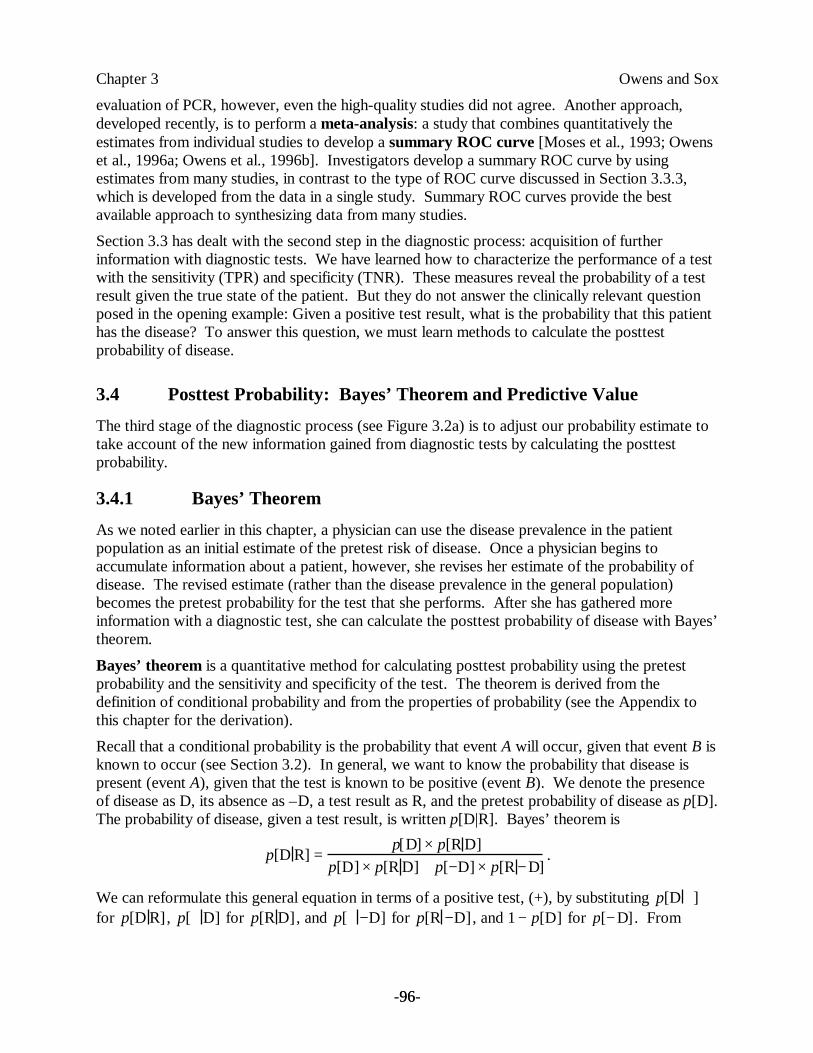
Recall that a conditional probability is the probability that event A will occur, given that event B isknown to occur (see Section 3.2). In general, we want to know the probability that disease ispresent (event A), given that the test is known to be positive (event B). We denote the presenceof disease as D, its absence as –D, a test result as R, and the pretest probability of disease as p[D].The probability of disease, given a test result, is written p[D|R]. Bayes’ theorem is
p[D R] = p[D] ×p[R D]p[D] ×p[R D] + p[− D] ×p[R − D]
.
We can reformulate this general equation in terms of a positive test, (+), by substituting p[D + ]for p[D R], p[+ D] for p[R D], and p[+ − D] for p[R − D], and 1 − p[D] for p[− D] . From
Chapter 3 Owens and Sox
-97-97
Section 3.3, recall that p[+ D] = TPR and p[+ − D] = FPR . Substitution provides Bayes’theorem for a positive test:
p[D + ] = p[D] ×TPRp[D] ×TPR + (1 − p[D]) ×FPR
.
We can use a similar derivation to develop Bayes’ theorem for a negative test:
p[D − ] = p[D] ×FNRp[D]×FNR + (1 − p[D]) ×TNR
.
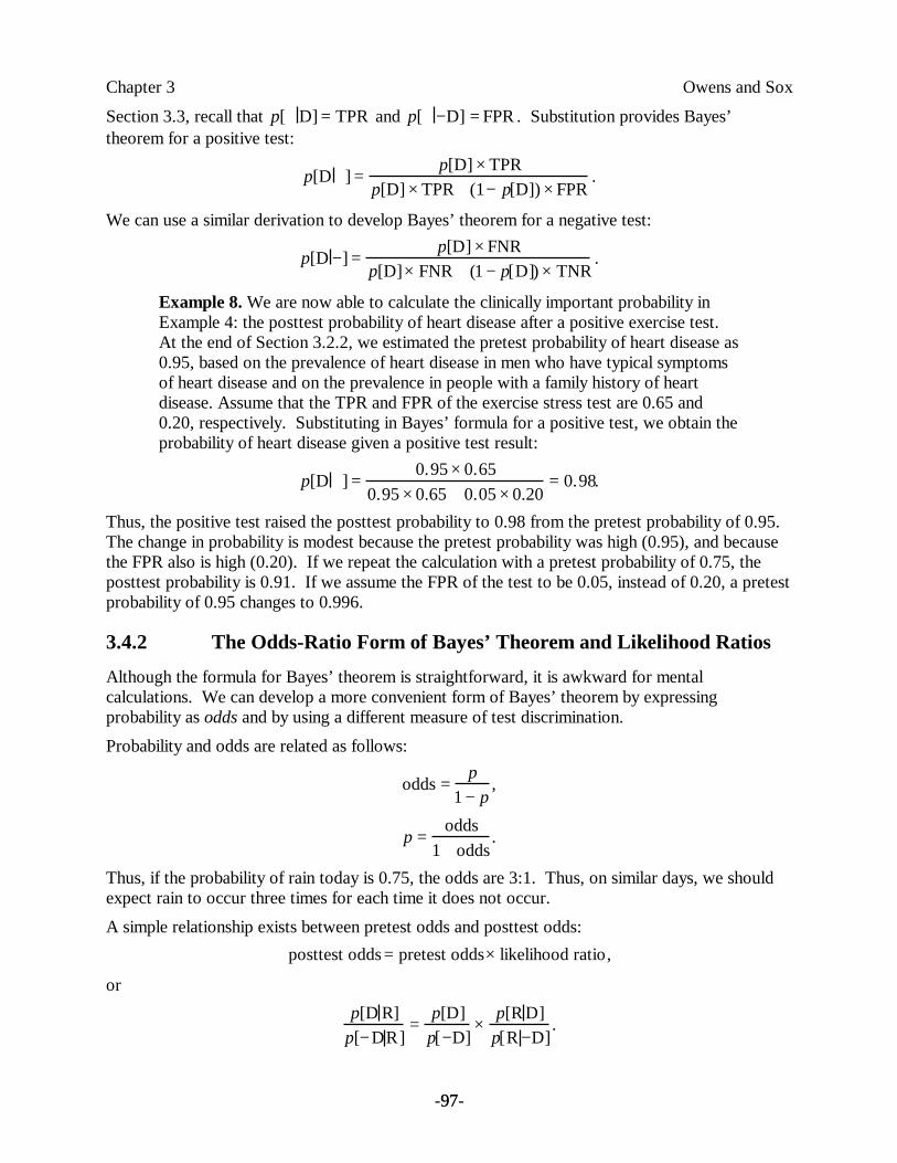
Example 8. We are now able to calculate the clinically important probability inExample 4: the posttest probability of heart disease after a positive exercise test.At the end of Section 3.2.2, we estimated the pretest probability of heart disease as0.95, based on the prevalence of heart disease in men who have typical symptomsof heart disease and on the prevalence in people with a family history of heartdisease. Assume that the TPR and FPR of the exercise stress test are 0.65 and0.20, respectively. Substituting in Bayes’ formula for a positive test, we obtain theprobability of heart disease given a positive test result:
p[D + ] = 0.95 ×0.650.95 ×0.65 + 0.05 ×0.20
= 0.98.
Thus, the positive test raised the posttest probability to 0.98 from the pretest probability of 0.95.The change in probability is modest because the pretest probability was high (0.95), and becausethe FPR also is high (0.20). If we repeat the calculation with a pretest probability of 0.75, theposttest probability is 0.91. If we assume the FPR of the test to be 0.05, instead of 0.20, a pretestprobability of 0.95 changes to 0.996.
3.4.2 The Odds-Ratio Form of Bayes’ Theorem and Likelihood Ratios
Although the formula for Bayes’ theorem is straightforward, it is awkward for mentalcalculations. We can develop a more convenient form of Bayes’ theorem by expressingprobability as odds and by using a different measure of test discrimination.
Probability and odds are related as follows:
odds = p1 − p
,
p = odds1 + odds
.
Thus, if the probability of rain today is 0.75, the odds are 3:1. Thus, on similar days, we shouldexpect rain to occur three times for each time it does not occur.
A simple relationship exists between pretest odds and posttest odds:posttest odds= pretest odds× likelihood ratio,
or
p[D R]p[− DR]
= p[D]p[ − D]
× p[R D]p[R − D]
.
Chapter 3 Owens and Sox
-98-98
This equation is the odds-ratio form of Bayes’ theorem.7 It can be derived in a straightforwardfashion from the definitions of Bayes’ theorem and of conditional probability that we providedearlier. Thus, to obtain the posttest odds, we simply multiply the pretest odds by the likelihoodratio (LR) for the test in question.
The LR of a test combines the measures of test discrimination discussed earlier to give onenumber that characterizes the discriminatory power of a test, defined as:
LR = p[R D]p[R − D]
.
or,
LR = probability of result in diseased peopleprobability of result in nondiseased people
.
The LR indicates the amount that the odds of disease change based on the test result. We can usethe LR to characterize clinical findings (such as a swollen leg) or a test result. We describe eitherby two likelihood ratios: one corresponding to a positive test result (or the presence of a finding),and the other corresponding to a negative test (or the absence of a finding). These ratios areabbreviated LR+ and LR–, respectively.
LR + = probability that test is positive in diseased peopleprobability that test is positive in nondiseased people
= TPRFPR
.
In a test that discriminates well between disease and nondisease, the TPR will be high, the FPRwill be low, and thus LR+ will be much greater than one. A LR of 1 means the probability of atest result is the same in diseased and nondiseased individuals; the test has no value. Similarly,
LR − = probability that test is negative in diseased peopleprobability that test is negative in nondiseased people
= FNRTNR
.
A desirable test will have a low FNR and a high TNR; therefore, the LR– will be much less than1.
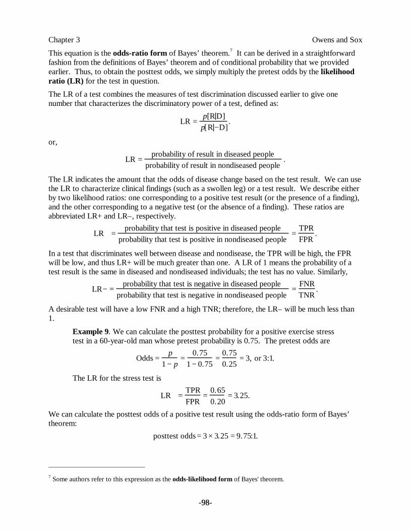
Example 9. We can calculate the posttest probability for a positive exercise stresstest in a 60-year-old man whose pretest probability is 0.75. The pretest odds are
Odds = p1 − p
= 0.751 − 0.75
= 0.750.25
= 3, or 3:1.
The LR for the stress test is
LR+ = TPRFPR
= 0.650.20
= 3.25.
We can calculate the posttest odds of a positive test result using the odds-ratio form of Bayes’theorem:
posttest odds= 3 ×3.25 = 9.75:1.
7 Some authors refer to this expression as the odds-likelihood form of Bayes' theorem.
Chapter 3 Owens and Sox
-99-99
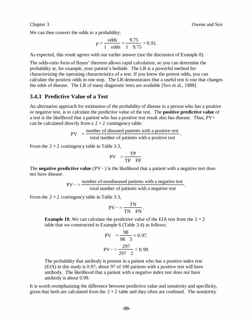
We can then convert the odds to a probability:
p = odds1 + odds
= 9.751 + 9.75
= 0.91.
As expected, this result agrees with our earlier answer (see the discussion of Example 8).
The odds-ratio form of Bayes’ theorem allows rapid calculation, so you can determine theprobability at, for example, your patient’s bedside. The LR is a powerful method forcharacterizing the operating characteristics of a test: If you know the pretest odds, you cancalculate the posttest odds in one step. The LR demonstrates that a useful test is one that changesthe odds of disease. The LR of many diagnostic tests are available [Sox et al., 1988].
3.4.3 Predictive Value of a Test
An alternative approach for estimation of the probability of disease in a person who has a positiveor negative test, is to calculate the predictive value of the test. The positive predictive value ofa test is the likelihood that a patient who has a positive test result also has disease. Thus, PV+can be calculated directly from a 2 ×2 contingency table:
PV+ = number of diseased patients with a positive testtotal number of patients with a positive test
.
From the 2 ×2 contingency table in Table 3.3,
PV+ = TPTP + FP
.
The negative predictive value (PV− ) is the likelihood that a patient with a negative test doesnot have disease:
PV− = number of nondiseased patients with a negative testtotal number of patients with a negative test
.
From the 2 ×2 contingency table in Table 3.3,
PV− = TNTN + FN
.
Example 10. We can calculate the predictive value of the EIA test from the 2 ×2table that we constructed in Example 6 (Table 3.4) as follows:
PV+ = 9898 + 3
= 0.97.
PV− = 297297 + 2
= 0.99.
The probability that antibody is present in a patient who has a positive index test(EIA) in this study is 0.97; about 97 of 100 patients with a positive test will haveantibody. The likelihood that a patient with a negative index test does not haveantibody is about 0.99.
It is worth reemphasizing the difference between predictive value and sensitivity and specificity,given that both are calculated from the 2 ×2 table and they often are confused. The sensitivity
Chapter 3 Owens and Sox
-100-100
and specificity give the probability of a particular test result in a patient who has a particulardisease state. The predictive value gives the probability of true disease state once the patient’stest result is known.
The positive predictive value calculated from Table 3.4 is 0.97, so we expect 97 of 100 patientswith a positive index test actually to have antibody. Yet, in Example 1, we found that less thanone of 10 patients with a positive test were expected to have antibody. What explains thediscrepancy in these examples? The sensitivity and specificity (and therefore, the LRs) in the twoexamples are identical. The discrepancy is due to an extremely important and often overlookedcharacteristic of predictive value: The predictive value of a test depends on the prevalence ofdisease in the study population (the prevalence can be calculated as TP + FN divided by the totalnumber of patients in the 2 ×2 table). The predictive value cannot be generalized to a newpopulation, because the prevalence of disease may differ between the two populations.
The difference in predictive value of the EIA in Example 1 and in Example 6 is due to a differencein the prevalence of disease in the examples. The prevalence of antibody was given as 0.001 inExample 1, and as 0.25 in Example 6. These examples should remind us that the positivepredictive value is not an intrinsic property of a test. Rather, it represents the posttest probabilityof disease only when the prevalence is identical to that in the 2 ×2 contingency table from whichthe positive predictive value was calculated. Bayes’ theorem provides a method for calculation ofthe posttest probability of disease for any prior probability. For that reason, we prefer the use ofBayes’ theorem to calculate the posttest probability of disease.
3.4.4 Implications of Bayes’ Theorem
In this section, we explore the implications of Bayes’ theorem for test interpretation. These ideasare extremely important, yet they often are misunderstood.
Figures 3.5(a) and 3.5(b) illustrate one of the most essential concepts in this chapter: The posttestprobability of disease increases as the pretest probability of disease increases. We producedFigure 3.5(a) by calculating the posttest probability after a positive test result for all possiblepretest probabilities of disease. We derived similarly Figure 3.5(b) for a negative test result.
The 45-degree line in each figure denotes a test in which the pretest and posttest probability areequal (LR = 1)— a test that is useless. The curve in Figure 3.5(a) relates pretest and posttestprobabilities in a test with a sensitivity and specificity of 0.9. Note that, at low pretestprobabilities, the posttest probability after a positive test result is much higher than is the pretestprobability. At high pretest probabilities, the posttest probability is only slightly higher than thepretest probability.
Figure 3.5(b) shows the relationship between the pretest and posttest probabilities after a negativetest result. At high pretest probabilities, the posttest probability after a negative test result ismuch lower than is the pretest probability. A negative test, however, has little effect on theposttest probability if the pretest probability is low.
________________________________________
Insert Figure 3.5 About Here
________________________________________
Chapter 3 Owens and Sox
-101-101
This discussion emphasizes a key idea of this chapter: The interpretation of a test result dependson the pretest probability of disease. If the pretest probability is low, a positive test result has alarge effect, and a negative test result has a small effect. If the pretest probability is high, apositive test result has a small effect, and a negative test result has a large effect. In other words,when the clinician is almost certain of the diagnosis prior to testing (pretest probability nearly 0 ornearly 1), a confirmatory test has little effect on the posterior probability (see Example 8). If thepretest probability is intermediate or if the result contradicts a strongly held clinical impression,the test result will have a large effect on the posttest probability.
Note from Figure 3.5(a) that, if the pretest probability is very low, a positive test result can raisethe posttest probability into only the intermediate range. Assume that Figure 3.5(a) represents therelationship between the pretest and posttest probabilities for the exercise stress test. If theclinician believes the pretest probability of coronary-artery disease is 0.1, the posttest probabilitywill be about 0.5. Although there has been a large change in the probability, the posttestprobability is in an intermediate range, which leaves considerable uncertainty about the diagnosis.Thus, if the pretest probability is low, it is unlikely that a positive test result will raise theprobability of disease sufficiently for the clinician to make that diagnosis with confidence. Anexception to this statement occurs when a test has a very high specificity (or large LR+); forexample, HIV antibody tests have a specificity greater than 0.99, and therefore a positive test isconvincing. Similarly, if the pretest probability is very high, it is unlikely that a negative test resultwill lower the posttest probability sufficiently to exclude a diagnosis.
Figure 3.6 illustrates another important concept: Test specificity affects primarily theinterpretation of a positive test; test sensitivity affects primarily the interpretation of a negativetest. In both parts a and b of Figure 3.6, the top family of curves corresponds to positive testresults, and the bottom family to negative test results. Figure 3.6(a) shows the posttestprobabilities for tests with varying specificities (TNR). Note that changes in the specificityproduce large changes in the top family of curves (positive test results), but have little effect onthe lower family of curves (negative test results). That is, an increase in the specificity of a testmarkedly changes the posttest probability if the test is positive, but has relatively little effect onthe posttest probability if the test is negative. Thus, if you are trying to rule in a diagnosis,8 youshould choose a test with high specificity, or a high LR+. Figure 3.6(b) shows the posttestprobabilities for tests with varying sensitivities. Note that changes in sensitivity produce largechanges in the bottom family of curves (negative test results), but have little effect on the topfamily of curves. Thus, if you are trying to exclude a disease, choose a test with a high sensitivity,or a high LR–.
8 In medicine, to rule in a disease is to confirm that the patient does have the disease; to rule out a disease is toconfirm that the patient does not have the disease. A doctor who strongly suspects that her patient has a bacterialinfection orders a culture to rule in her diagnosis. Another doctor is almost certain that his patient has a simplesore throat, but orders a culture to rule out streptococcal infection (strep throat). This terminology oversimplifies adiagnostic process that is probabilistic. Diagnostic tests rarely, if ever, rule in or rule out a disease; rather, the testsraise or lower the probability of disease.
Chapter 3 Owens and Sox
-102-102
________________________________________
Insert Figure 3.6 About Here
________________________________________
3.4.5 Cautions in the Application of Bayes’ Theorem
Bayes’ theorem provides a powerful method for calculating posttest probability. You should beaware, however, of the possible errors you can make when you use it. Common problems areinaccurate estimation of pretest probability, faulty application of test-performance measures, andviolation of the assumptions of conditional independence and of mutual exclusivity.
Bayes’ theorem provides a means to adjust an estimate of pretest probability to take account ofnew information. The accuracy of the calculated posttest probability is limited, however, by theaccuracy of the estimated pretest probability. Accuracy of estimated prior probability is increasedby proper use of published prevalence rates, heuristics, and clinical prediction rules. In a decisionanalysis, as we shall see, a range of prior probability often is sufficient. Nonetheless, if thepretest-probability assessment is unreliable, Bayes’ theorem will be of little value.
A second potential mistake that you can make when using Bayes’ theorem is to apply publishedvalues for the test sensitivity and specificity, or LRs, without paying attention to the possibleeffects of bias in the studies in which the test performance was measured (see Section 3.3.5).With certain tests, the LRs may differ depending on the pretest odds, in part because differencesin pretest odds may reflect differences in the spectrum of disease in the population.
A third potential problem arises when you use Bayes’ theorem to interpret a sequence of tests. Ifa patient undergoes two tests in sequence, you can use the posttest probability after the first testresult, calculated with Bayes’ theorem, as the pretest probability for the second test. Then, youuse Bayes’ theorem a second time, to calculate the posttest probability after the second test. Thisapproach is valid, however, only if the two tests are conditionally independent. Tests for the samedisease are conditionally independent when the probability of a particular result on the secondtest does not depend on the result of the first test, given (conditioned on) the disease state.Expressed in conditional-probability notation, for the case in which the disease is present,
]present disease and positive first test positive test second[p
present] disease and negative first test positive test second[p=present]. disease positive test second[p=
If the conditional independence assumption is satisfied, the posttest odds = pretest odds × LR1 ×LR2. If you apply Bayes’ theorem sequentially in situations in which conditional independence isviolated, you will obtain inaccurate posttest probabilities.
The fourth common problem arises when you assume that all test abnormalities result from one(and only one) disease process. The Bayesian approach, as we have described it, generallypresumes that the diseases under consideration are mutually exclusive. If they are not, Bayesianupdating must be applied with great care.

Chapter 3 Owens and Sox
-103-103
We have shown how to calculate posttest probability. In Section 3.5, we turn to the problem ofdecision making when the outcomes of a physician’s actions (for example, of treatments) areuncertain.
3.5 Expected-Value Decision Making
Medical decision-making problems often cannot be solved by reasoning based onpathophysiology. For example, clinicians need a method for choosing among treatments when theoutcome of the treatments is unpredictable, as are the results of a surgical operation. You can usethe ideas developed in the preceding sections to solve such difficult decision problems. Here, wewill discuss two methods: the decision tree, a method for representing and comparing theexpected outcomes of each decision alternative; and the threshold probability, a method fordeciding whether new information can change a management decision. These techniques help youto clarify the decision problem and thus to choose the alternative that is most likely to help thepatient.
3.5.1 Comparison of Uncertain Prospects
Like those of most biological events, the outcome of an individual’s illness is unpredictable. Howcan a physician determine which course of action has the greatest chance of success?
Example 11. There are two available therapies for a fatal illness. The length of apatient’s life after either therapy is unpredictable, as illustrated by the frequencydistribution shown in Figure 3.7 and summarized in Table 3.5. Each therapy isassociated with uncertainty: Regardless of which therapy a patient receives, he willdie by the end of the fourth year, but there is no way to know which year will bethe patient’s last. Figure 3.7 shows that survival until the fourth year is more likelywith therapy B, but the patient might die in the first year with therapy B or mightsurvive to the fourth year with therapy A.
________________________________________
Insert Figure 3.7 About Here
________________________________________
________________________________________
Insert Table 3.5 About Here
________________________________________
Which of the two therapies is preferable? This example demonstrates a significant fact: A choiceamong therapies is a choice among gambles (that is, situations in which chance determines theoutcomes). How do we usually choose among gambles? More often than not, we rely onhunches or on a sixth sense. How should we choose among gambles? We propose a method forchoosing called expected-value decision making: We characterize each gamble by a number,
Chapter 3 Owens and Sox
-104-104
and we use that number to compare the gambles.9 In Example 11, therapy A and therapy B areboth gambles with respect to duration of life after therapy. We want to assign a measure (ornumber) to each therapy that summarizes the outcomes such that we can decide which therapy ispreferable.
The ideal criterion for choosing a gamble should be a number that reflects preferences (inmedicine, often the patient’s preferences) for the outcomes of the gamble. Utility is the namegiven to a measure of preference that has a desirable property for decision making: The gamblewith the highest utility should be preferred. We shall discuss utility briefly (Section 3.5.4), butyou can pursue this topic and the details of decision analysis in other textbooks (see theSuggested Readings at the end of this chapter).10 We use the average duration of life aftertherapy (survival) as a criterion for choosing among therapies; remember that this model isoversimplified, used here for discussion only. Later, we will consider other factors, such as thequality of life.
Because we cannot be sure of the duration of survival in any given patient, we characterize atherapy by the mean survival (average length of life) that would be observed in a large number ofpatients after they were given the therapy. The first step we take in calculating the mean survivalfor a therapy is to divide the population receiving the therapy into groups of patients who havesimilar survival rates. Then, we multiply the survival time in each group11 by the fraction of thetotal population in that group. Finally, we sum these products over all possible survival values.
We can perform this calculation for the therapies in Example 11. Mean survival for therapy A =(0.2 ×1.0) + (0.4 ×2.0) + (0.3×3.0) + (0.1×4.0) = 2.3 years. Mean survival for therapy B =(0.05 ×1.0) + (0.15×2.0) + (0.45×3.0) + (0.35×4.0) = 3.1 years.
Survival after a therapy is under the control of chance. Therapy A is a gamble characterized by anaverage survival equal to 2.3 years. Therapy B is a gamble characterized by an average survival of3.1 years. If length of life is our criterion for choosing, we should select therapy B.
3.5.2 Representation of Choices with Decision Trees
The choice between therapies A and B is represented diagrammatically in Figure 3.8. Events thatare under the control of chance can be represented by a chance node. By convention, a chancenode is shown as a circle from which several lines emanate. Each line represents one of thepossible outcomes. Associated with each line is the probability of the outcome occurring. For asingle patient, only one outcome can occur. Some physicians object to using probability for justthis reason: “You cannot rely on population data, because each patient is an individual.” In fact,we often must use the frequency of the outcomes of many patients experiencing the same event toinform our opinion about what might happen to an individual. From these frequencies, we canmake patient-specific adjustments and thus estimate the probability of each outcome at a chancenode.
9 Expected-value decision making had been used in many fields before it was first applied to medicine.10 A more general term for expected-value decision making is expected utility decision making. Because a fulltreatment of utility is beyond the scope of this chapter, we have chosen to use the term expected value.11 For this simple example, death during an interval is assumed to occur at the end of the year.
Chapter 3 Owens and Sox
-105-105
A chance node can represent more than just an event governed by chance. The outcome of achance event, unknowable for the individual, can be represented by the expected value at thechance node. The concept of expected value is important and is easy to understand. We cancalculate the mean survival that would be expected if many patients had the treatment depicted bythe chance node in Figure 3.8. This average length of life is called the expected survival, or, moregenerally, the expected value of the chance node. We calculate expected value at a chance nodeby the process just described: We multiply the survival value associated with each possibleoutcome by the probability that that outcome will occur. We then sum the product of probabilitytimes survival over all outcomes. Thus, if several hundred patients were assigned to receive eithertherapy A or therapy B, the expected survival would be 2.3 years for therapy A and 3.1 years fortherapy B.
________________________________________
Insert Figure 3.8 About Here
________________________________________
We have just described the basis of expected-value decision making. The term expected value isused to characterize a chance event, such as the outcome of a therapy. If the outcomes of atherapy are measured in units of duration of survival, units of sense of well-being, or dollars, thetherapy is characterized by the expected duration of survival, expected sense of well-being, orexpected monetary cost that it will confer on or incur for the patient, respectively.
To use expected-value decision making, we follow this strategy when there are therapy choiceswith uncertain outcomes: (1) calculate the expected value of each decision alternative, then (2)pick the alternative with the highest expected value.
3.5.3 Performance of a Decision Analysis
We clarify the concepts of expected-value decision making by discussing an example.
There are four steps in decision analysis:
1. Create a decision tree; this step is the most difficult, because it requires formulating thedecision problem, assigning probabilities, and measuring outcomes.
2. Calculate the expected value of each decision alternative.
3. Choose the decision alternative with the highest expected value.
4. Use sensitivity analysis to test the conclusions of the analysis.
Many health professionals balk when they first learn about the technique of decision analysis,because they recognize the opportunity for error in assigning values to both the probabilities andthe utilities in a decision tree. They reason that the technique encourages decision making basedon small differences in expected values that are estimates at best. The defense against thisconcern, which also has been recognized by decision analysts, is the technique known assensitivity analysis. We shall discuss this important fourth step in decision analysis in Section3.5.5.
The first step in decision analysis is to create a decision tree that represents the decision problem.Consider the following clinical problem.
Chapter 3 Owens and Sox
-106-106
Example 12. The patient is Mr. Danby, a 66-year-old man who has been crippledwith arthritis of both knees so severely that while he can get about the house withthe aid of two canes, he must otherwise use a wheelchair. His other major healthproblem is emphysema, a disease in which the lungs lose their ability to exchangeoxygen and carbon dioxide between blood and air, which in turn causes shortnessof breath (dyspnea). He is able to breathe comfortably when he is in a wheelchair,but the effort of walking with canes makes him breathe heavily and feeluncomfortable. Several years ago, he seriously considered knee-replacementsurgery but decided against it, largely because his internist told him that there wasa serious risk that he would not survive the operation because of his lung disease.Recently, however, Mr. Danby’s wife had a stroke and was partially paralyzed; shenow requires a degree of assistance that the patient cannot supply given his presentstate of mobility. He tells his doctor that he is reconsidering knee-replacementsurgery.
Mr. Danby’s internist is familiar with decision analysis. She recognizes that thisproblem is filled with uncertainty: Mr. Danby’s ability to survive the operation is indoubt, and the surgery sometimes does not restore mobility to the degree requiredby this patient. Furthermore, there is a small chance that the prosthesis (theartificial knee) will become infected, and Mr. Danby then would have to undergo asecond risky operation to remove it. After removal of the prosthesis, Mr. Danbywould never again be able to walk, even with canes. The possible outcomes ofknee replacement include death from the first procedure, and death from a secondmandatory procedure if the prosthesis becomes infected (which we will assumeoccurs in the immediate postoperative period, if it occurs at all). Possiblefunctional outcomes include recovery of full mobility, or continued, andunchanged, poor mobility. Should Mr. Danby choose to undergo knee-replacementsurgery or should he accept the status quo?
Using the conventions of decision analysis, the internist sketches the decision tree shown in Figure3.9. According to these conventions, a square box denotes a decision node, and each lineemanating from a decision node represents an action that could be taken.
According to the methods of expected-value decision making, the internist first must assign aprobability to each branch of each chance node. To accomplish this task, the internist asks severalorthopedic surgeons for their estimates of the chance of recovering full function after surgery( p[full recovery] = 0.60) and the chance of developing infection in the prosthetic joint( p[ infection] = 0.05). She uses her subjective estimate of the probability that the patient will dieduring or immediately after knee surgery ( p[operative death] = 0.05).
________________________________________
Insert Figure 3.9 About Here
________________________________________
Next, she must assign a value to each outcome. To accomplish this task, she first lists theoutcomes. As you can see from Table 3.6, the outcomes differ in two dimensions: length of life(survival) and quality of life (functional status). To characterize each outcome accurately, the
Chapter 3 Owens and Sox
-107-107
internist must develop a measure that takes into account these two dimensions. Simply usingduration of survival is inadequate because Mr. Danby values 5 years of good health more than hevalues 10 years of poor health. The internist can account for this tradeoff factor by convertingoutcomes with two dimensions into outcomes with a single dimension: duration of survival ingood health. The resulting measure is called a quality-adjusted life year (QALY).12 She canconvert years in poor health into years in good health by asking Mr. Danby to indicate the shortestperiod in good health (full mobility) that he would accept in return for his full expected lifetime(10 years) in a state of poor health (status quo). Thus, she asks Mr. Danby, “Many people saythey would be willing to accept a shorter life in excellent health in preference to a longer life withsignificant disability. In your case, how many years with normal mobility do you feel is equivalentin value to 10 years in your current state of disability?” She asks him this question for eachoutcome. The patient’s responses are shown in the third column of Table 3.6. The patientdecides that 10 years of limited mobility are equivalent to 6 years of normal mobility, whereas 10years of wheelchair confinement are equivalent to only 3 years of full function. Figure 3.10 showsthe final decision tree— complete with probability estimates and utility values for each outcome.13
________________________________________
Insert Table 3.6 About Here
________________________________________
________________________________________
Insert Figure 3.10 About Here
________________________________________
The second task that the internist must undertake is to calculate the expected value, in healthyyears, of surgery and of no surgery. She calculates the expected value at each chance node,moving from right (the tips of the tree) to left (the root of the tree). Let us consider, for example,the expected value at the chance node representing the outcome of surgery to remove an infectedprosthesis (Node A in Figure 3.10). The calculation requires three steps:
1. Calculate the expected value of operative death after surgery to remove an infectedprosthesis. Multiply the probability of operative death (0.05) by the QALY of theoutcome— death (0 years): 0.05 ×0 = 0 (QALY).
2. Calculate the expected value of surviving surgery to remove an infected knee prosthesis.Multiply the probability of surviving the operation (0.95) by the number of healthy yearsequivalent to 10 years of being wheelchair bound (3 years): 0.95 ×3 = 2.85 (QALY).
12 Quality-adjusted life years commonly are used as measures of utility (value) in medical decision analysis and inhealth-policy analysis (see, for example, the discussion of cost-effectiveness analysis in Chapter 8).13 In a more sophisticated decision analysis, the physician also would adjust the utility values of outcomes thatrequire surgery to account for the pain and inconvenience associated with surgery and rehabilitation.

Chapter 3 Owens and Sox
-108-108
3. Add the expected values calculated in step 1 (0 QALY) and step 2 (2.85 QALY) to obtainthe expected value of developing an infected prosthesis: 0 + 2.85 = 2.85 (QALY).
Similarly, the expected value at chance node B is calculated: (0.6 ×10) + (0.4×6) = 8.4(QALY). To obtain the expected value of surviving knee-replacement surgery (Node C), sheproceeds as follows:
1. Multiply the expected value of an infected prosthesis (already calculated as 2.85 QALY)by the probability that the prosthesis will become infected (0.05): 2.85 ×0.05 = 0.143(QALY).
2. Multiply the expected value of never developing an infected prosthesis (already calculatedas 8.4 QALY) by the probability that the prosthesis will not become infected (0.95): 8.4×0.95 = 7.98 (QALY).
3. Add the expected values calculated in step 1 (0.143 QALY) and step 2 (7.98 QALY) toget the expected value of surviving knee replacement surgery: 0.143 + 7.98 = 8.123(QALY).
The physician performs this process, called averaging out at chance nodes, for node D as well,working back to the root of the tree, until the expected value of surgery has been calculated. Theoutcome of the analysis is as follows. For surgery, Mr. Danby’s average life expectancy,measured in years of normal mobility, is 7.7. What does this value mean? It does not mean that,by accepting surgery, Mr. Danby is guaranteed 7.7 years of mobile life. One look at the decisiontree will show that some patients die in surgery, some develop infection, and some do not gainany improvement in mobility after surgery. So, an individual patient has no guarantees.However, if the physician had 100 similar patients who underwent the surgery, the averagenumber of mobile years would be 7.7. We can understand what this value means for Mr. Danbyonly by examining the alternative: no surgery.
In the analysis for no surgery, the average length of life, measured in years of normal mobility, is6.0, which Mr. Danby considered equivalent to 10 years of continued poor mobility. Not allpatients will experience this outcome; some who have poor mobility will live longer than, andsome will live less than, 10 years. The average length of life, however, expressed in years ofnormal mobility, will be 6. Because 6.0 is less than 7.7, on average the surgery will provide anoutcome with higher value to the patient. Thus, the internist recommends performing the surgery.
The key insight of expected-value decision making should be clear from this example: Given theunpredictable outcome in an individual, the best choice for the individual is the alternative thatgives the best result on the average in similar patients. Decision analysis can help the physician toidentify the therapy that will give the best results when averaged over many similar patients. Thedecision analysis is tailored to a specific patient in that both the utility functions and theprobability estimates are adjusted to the individual. Nonetheless, the results of the analysisrepresent the outcomes that would occur on the average in a population of patients who havesimilar utilities and for whom uncertain events have similar probabilities.
3.5.4 Representation of Patients’ Preferences with Utilities
In Section 3.5.3, we introduced the concept of QALYs, because length of life is not the onlyoutcome about which patients care. Patients’ preferences for a health outcome may depend onthe length of life with the outcome, on the quality of life with the outcome, and on the risk
Chapter 3 Owens and Sox
-109-109
involved in achieving the outcome (for example, a cure for cancer might require a risky surgicaloperation). How can we incorporate these elements into a decision analysis? To do so, we canrepresent patients’ preferences with utilities. The utility of a health state is a quantitative measureof the desirability of a health state, from the patient’s perspective. Utilities are typically expressedon a 0-to-1 scale, where 0 represents death and 1 represents ideal health. For example, a study ofpatients who had chest pain (angina) with exercise rated the utility of mild, moderate, and severeangina as 0.95, 0.92, and 0.82 [Nease et al., 1995]. There are several methods for assessingutilities.
The standard-gamble technique has the strongest theoretical basis as shown by Von Neumannand Morgenstern and described in Sox and colleagues [Sox et al., 1988] of the variousapproaches to utility assessment. To illustrate use of the standard gamble, suppose that we seekto assess a person’s utility for the health state of asymptomatic HIV infection. To use thestandard gamble, we ask our subject to compare the desirability of asymptomatic HIV infection tothose of two other health states whose utility we know, or can assign. Often, we use ideal health(assigned a utility of 1) and immediate death (assigned a utility of 0) for the comparison of healthstates. We then ask our subject to choose between asymptomatic HIV infection, and a gamblewith a chance of ideal health or immediate death. We vary the probability of ideal health andimmediate death systematically until the subject is indifferent between asymptomatic HIVinfection and the gamble. For example, a subject might be indifferent when the probability of idealhealth is 0.8 and the probability of death is 0.2. At this point of indifference, the utility of thegamble and that of asymptomatic HIV infection are equal, a key relationship that allows us tocalculate the utility of the gamble as the weighted average of the utilities of each outcome of thegamble [(1 × 0.8) + (0 × 0.2)] = 0.8. So, in this example, the utility of asymptomatic HIVinfection is 0.8. Use of the standard gamble enables an analyst to assess the utility of outcomesthat differ in length or quality of life. Because the standard gamble involves chance events, it alsoassesses a person’s willingness to take risks— called the person’s risk attitude.
A second common approach to utility assessment is the time-tradeoff technique [Sox et al.,1988; Torrance & Feeny, 1989]. To assess the utility of asymptomatic HIV infection using thetime-tradeoff technique, we ask a person to determine the length of time in a better state of health(usually ideal health or best attainable health) that he would find equivalent to a longer period oftime with asymptomatic HIV infection. For example, if our subject says that 8 months of life withideal health was equivalent to 12 months of life with asymptomatic HIV infection, then wecalculate the utility of asymptomatic HIV infection as 8 ÷ 12 = 0.67. The time-tradeoff techniqueprovides a convenient method for valuing outcomes that accounts for gains (or losses) in bothlength and quality of life. However, because the time tradeoff does not include gambles, it doesnot assess a person’s risk attitude. Perhaps the strongest assumption underlying the use of thetime tradeoff as a measure of utility is that people are risk neutral. A risk-neutral decision makeris indifferent between the expected value of a gamble and the gamble itself. For example, a risk-neutral decision maker would be indifferent between the choice of living 20 years (for certain) andthat of taking a gamble with a 50 percent chance of living 40 years and a 50 percent chance ofimmediate death (which has an expected value of 20 years). In practice, of course, few people arerisk neutral. Nonetheless, the time-tradeoff technique is used frequently to value health outcomesbecause it is relatively easy to understand.
Several other approaches are available to value health outcomes. To use the visual-analog scale,a person simply rates the quality of life with a health outcome (for example, asymptomatic HIV

Chapter 3 Owens and Sox
-110-110
infection) on a scale from 0 to 100. Although the visual-analog scale is easy to explain and use, ithas no theoretical justification as a valid measure of utility. However, ratings with the visual-analog scale correlate modestly well with utilities assessed by the standard gamble and timetradeoff. For a demonstration of the use of standard gambles, time-tradeoffs, and the visual-analog scale to assess utilities in patients with angina, see Nease and colleagues [Nease et al.,1995]. Other approaches to valuing health outcomes include the Quality of Well Being Scale, theHealth Utilities Index, and the EuroQoL [Gold et al., 1996, Chapter 4]. Each of theseinstruments assesses how people value health outcomes, and therefore may be appropriate for usein decision analyses or cost-effectiveness analyses.
In summary, we can use utilities to represent how patients value complicated health outcomes thatdiffer in length and quality of life, and in riskiness. Computer-based tools with an interactiveformat, are now available for assessing utilities; they often include text and multimediapresentations that enhance patients’ understanding of the assessment tasks and of the healthoutcomes [Lenert et al., 1995; Nease & Owens, 1994; Sumner et al., 1991].
3.5.5 Performance of Sensitivity Analysis
Sensitivity analysis is a test of the validity of the conclusions of an analysis over a wide range ofassumptions about the probabilities and the values, or utilities. The probability of an outcome at achance node may be the best estimate that is available, but there often is a wide range ofreasonable probabilities that a physician could use with nearly equal confidence. We usesensitivity analysis to answer this question: Do my conclusions regarding the preferred choicechange when the probability and outcome estimates are assigned values that lie within areasonable range?
The knee-replacement decision in Example 12 illustrates the power of sensitivity analysis. If theconclusions of the analysis (surgery is preferable to no surgery) remain the same despite a widerange of assumed values for the probabilities and outcome measures, the recommendation istrustworthy. Figures 3.11 and 3.12 show the expected survival in healthy years with surgery andwithout surgery under varying assumptions of the probability of operative death and theprobability of attaining perfect mobility, respectively. Each point (value) on these lines representsone calculation of expected survival using the tree in Figure 3.9. Figure 3.11 shows that expectedsurvival is higher with surgery over a wide range of operative mortality rates. Expected survivalis lower with surgery, however, when the operative mortality rate exceeds 25 percent. Figure3.12 shows the effect of varying the probability that the operation will lead to perfect mobility.The expected survival, in healthy years, is higher for surgery as long as the probability of perfectmobility exceeds 20 percent, a much lower figure than is expected from previous experience withthe operation. (In Example 12, the consulting orthopedic surgeons estimated the chance of fullrecovery at 60 percent). Thus, the internist can proceed with confidence to recommend surgery.Mr. Danby cannot be sure of a good outcome, but he has valid reasons for thinking that he ismore likely to do well with surgery than he is without it.
________________________________________
Insert Figure 3.11 About Here
________________________________________
Chapter 3 Owens and Sox
-111-111
________________________________________
Insert Figure 3.12 About Here
________________________________________
Another way to state the conclusions of a sensitivity analysis is to indicate the range ofprobabilities over which the conclusions apply. The point at which the two lines in Figure 3.11cross is the probability of operative death at which the two therapy options have the sameexpected survival. If expected survival is to be the basis for choosing therapy, the internist andthe patient should be indifferent between surgery and no surgery when the probability of operativedeath is 25 percent.14 When the probability is lower, they should select surgery. When it is higher,they should select no surgery.
3.5.6 Representation of Long-Term Outcomes with Markov Models
In Example 12, we evaluated Mr. Danby’s decision to have surgery to improve his mobility,which was compromised by arthritis. We assumed that each of the possible outcomes (fullmobility, poor mobility, death, and so on) would occur shortly after Mr. Danby took action on hisdecision. But what if we want to model events that might occur in the distant future? Forexample, a patient with HIV infection might develop AIDS 10 to 15 years after infection; thus, atherapy to prevent or delay the development of AIDS could affect events that occur 10 to 15years, or more, in the future. A similar problem arises in analyses of decisions regarding manychronic diseases: We must model events that occur over the lifetime of the patient. The decision-tree representation is convenient for decisions for which all outcomes occur during a short timehorizon, but it is not always sufficient for problems that include events that could occur in thefuture. How can we include such events in a decision analysis? The answer is to use Markovmodels [Beck & Pauker, 1983; Sonnenberg & Beck, 1993].
To build a Markov model, we first specify the set of health states that a person could experience(for example, Well, Cancer, and Death in Figure 3.13). We then specify the transitionprobabilities, which are the probabilities that a person will transit from one of these health statesto another during a specified time period. This period— often 1 month or 1 year— is the length ofthe Markov cycle. The Markov model then simulates the transitions among health states for aperson (or for a hypothetical cohort of people) for a specified number of cycles; by using aMarkov model, we can calculate the probability that a person will be in each of the health states atany time in the future.
________________________________________
Insert Figure 3.13 About Here
________________________________________
14 An operative mortality rate of 25 percent may seem high; however, this value is correct when we use QALYs asthe basis for choosing treatment. A decision maker performing a more sophisticated analysis could use a utilityfunction that reflects the patient’s aversion to risking death.

Chapter 3 Owens and Sox
-112-112
As an illustration, consider a simple Markov model that has three health states, Well, Cancer, andDeath (Figure 3.13). We have specified each of the transition probabilities in Table 3.7, for thecycle length of 1 year. Thus, we note from Table 3.7 that a person who is in the Well state willremain well with probability 0.9, will develop cancer with probability 0.06, and will die fromnoncancer causes with probability 0.04 during 1 year. The calculations for a Markov model areperformed by computer software. Based on the transition probabilities in Table 3.7, theprobabilities that a person remains well, develops cancer, or dies from noncancer causes over timeis shown in Table 3.8. We can also determine from a Markov model the expected length of timethat a person spends in each health state. Therefore, we can determine life expectancy, or quality-adjusted life expectancy, for any alternative represented by a Markov model.
________________________________________
Insert Table 3.7 About Here
________________________________________
________________________________________
Insert Table 3.8 About Here
________________________________________
In decision analyses that represent long-term outcomes, the analysts will often use a Markovmodel in conjunction with a decision tree to model the decision [Owens et al., 1995; Owens,Sanders et al., 1997; Salpeter et al., 1997]. The analyst models the effect of an intervention as achange in the probability of going from one state to another. For example, we could model acancer-prevention intervention (such as screening for breast cancer with mammography) as areduction in the transition probability from Well to Cancer in Figure 3.13. For further explanationof the use of Markov models, see the articles by Beck and Pauker [Beck & Pauker, 1983] and bySonnenberg and Beck [Sonnenberg & Beck, 1993].
3.6 The Decision Whether to Treat, Test, or Do Nothing
The physician who is evaluating a patient’s symptoms and suspects a disease must choose amongthe following actions:
1. Do nothing further (neither perform additional tests nor treat the patient).
2. Obtain additional diagnostic information (test) before choosing whether to treat or donothing.
3. Treat without obtaining more information.
When the physician knows the patient’s true state, testing is unnecessary, and the doctor needsonly to assess the tradeoffs among therapeutic options (as in Example 12). Learning the patient’strue state, however, may require costly, time-consuming, and often risky diagnostic proceduresthat may give misleading FP or FN results. Therefore, physicians often are willing to treat apatient even when they are not absolutely certain about a patient’s true state. There are risks inthis course: The physician may withhold therapy from a person who has the disease of concern, or
Chapter 3 Owens and Sox
-113-113
he may administer therapy to someone who does not have the disease yet may suffer undesirableside effects of therapy.
Deciding among treating, testing, and doing nothing sounds difficult, but you have already learnedall the principles that you need to solve this kind of problem. There are three steps:
1. Determine the treatment-threshold probability of disease.
2. Determine the pretest probability of disease.
3. Decide whether a test result could affect your decision to treat.
The treatment-threshold probability of disease is the probability of disease at which you shouldbe indifferent between treating and not treating [Pauker & Kassirer, 1980]. Below the treatmentthreshold, you should not treat. Above the treatment threshold, you should treat (Figure 3.14).
________________________________________
Insert Figure 3.14 About Here
________________________________________
Whether to treat when the diagnosis is not certain is a problem that you can solve with a decisiontree, such as the one shown in Figure 3.15. You can use this tree to learn the treatment-thresholdprobability of disease by leaving the probability of disease as an unknown, setting the expectedvalue of surgery equal to the expected value for medical (that is, nonsurgical, such as drugs orphysical therapy) treatment, and solving for the probability of disease. (In this example, surgerycorresponds to the “treat” branch of the tree in Figure 3.15, and nonsurgical interventioncorresponds to the “do not treat” branch.) Because you are indifferent between medical treatmentand surgery at this probability, it is the treatment-threshold probability. Using the tree completesstep 1. In practice, people often determine the treatment threshold intuitively rather thananalytically.
________________________________________
Insert Figure 3.15 About Here
________________________________________
An alternative approach to determination of the treatment threshold probability is to use theequation
p* = HH + B
where p*= the treatment threshold probability, H = the harm associated with treatment of anondiseased patient, and B = the benefit associated with treatment of a diseased patient [Pauker &Kassirer, 1980; Sox et al., 1988]. We define B as the difference between the utility (U) ofdiseased patients who are treated and diseased patients who are not treated [U(D, treat) – U(D,do not treat), as shown in Figure 3.15]. The utility of diseased patients who are treated should begreater than that of diseased patients who are not treated; therefore B is positive. We define H asthe difference in utility of nondiseased patients who are not treated and nondiseased patients whoare treated[U(–D, do not treat) – U(–D, treat), as shown in Figure 3.15]. The utility of
Chapter 3 Owens and Sox
-114-114
nondiseased patients who are not treated should be greater than that of nondiseased patients whoare treated; therefore H is positive. The equation for the treatment-threshold probability fits withour intuition: If the benefit of treatment is small and the harm of treatment is large, then thetreatment-threshold probability will be high. In contrast, if the benefit of treatment is large, andthe harm of treatment is small, the treatment threshold will be low.
Once you know the pretest probability, you know what to do in the absence of further informationabout the patient. If the pretest probability is below the treatment threshold, you should not treatthe patient. If the pretest probability is above the threshold, you should treat the patient. So youhave completed step 2.
One of the guiding principles of medical decision making is this: Do not order a test unless itcould change your management of the patient. In our framework for decision making, thisprinciple means that you should order a test only if the test result could cause the probability ofdisease to cross the treatment threshold. Thus, if the pretest probability is above the treatmentthreshold, a negative test result must lead to a posttest probability that is below the threshold.Conversely, if the pretest probability is below the threshold probability, a positive result must leadto a posttest probability that is above the threshold. In either case, the test result would alter yourdecision whether to treat the patient. This analysis completes step 3.
To decide whether a test could alter management, we simply use Bayes’ theorem. We calculatethe posttest probability following a test result that would move the probability of disease towardthe treatment threshold. If the pretest probability is above the treatment threshold, we calculatethe probability of disease if the test result is negative. If the pretest probability is below thetreatment threshold, we calculate the probability of disease if the test result is positive.
Example 13. You are a pulmonary medicine specialist. You suspect that a patientof yours has a pulmonary embolus (blood clot lodged in the vessels of the lungs).The usual approach is to do a radionuclide lung scan, a test in which tinyradioactive particles are injected into a vein. These particles flow into the smallvessels of the lung. A scanning device detects the radiation from the particles. Theparticles cannot go to a part of the lungs that is supplied by a vessel that is blockedby a blood clot. Unfortunately, there are other causes of blank areas in the scan,so that you cannot be sure that a blood clot is present when there is a blank area.Thus, if the scan is abnormal (shows a blank area), you must perform a definitivetest to confirm the diagnosis. Such a test is a pulmonary arteriogram, in whichradiopaque dye is injected into the arteries in the lung, and an X-ray image isobtained. The procedure involves further risk, discomfort, and substantial cost tothe patient. If the scan is negative, you do no further tests and do not treat thepatient.
To decide whether this strategy is correct, you take the following steps:
1. Determine the treatment-threshold probability of pulmonary embolus.
2. Estimate the pretest probability of pulmonary embolus.
3. Decide whether a test result could affect your decision to treat for an embolus.
First, assume you decide that the treatment threshold should be 0.10 in this patient. What does itmean to have a treatment-threshold probability equal to 0.10? If you could obtain no furtherinformation, you would treat for pulmonary embolus if the pretest probability was above 0.10

Chapter 3 Owens and Sox
-115-115
(that is, if you believed that there was greater than a one in 10 chance that the patient had anembolus), and would withhold therapy if the pretest probability was below 0.10. A decision totreat when the pretest probability is at the treatment threshold means that you are willing to treatnine patients without pulmonary embolus to be sure of treating one patient who has pulmonaryembolus. A relatively low treatment threshold is justifiable because treatment of a pulomonaryembolism with blood-thinning medication substantially reduces the high mortality of pulmonaryembolism, whereas there is only a relatively small danger (mortality of less than 1 percent) intreating someone who does not have pulmonary embolus. Because the benefit of treatment ishigh and the harm of treatment is low, the treatment-threshold probability will be low, asdiscussed earlier. You have completed step 1.
You estimate the pretest probability of pulmonary embolus to be 0.05, which is equal to a pretestodds of 0.053. Because the pretest probability is lower than the treatment threshold, you shoulddo nothing unless a positive lung-scan result could raise the probability of pulmonary embolus toabove 0.10. You have completed step 2.
To decide whether a test result could affect your decision to treat, you must decide whether apositive lung-scan result would raise the probability of pulmonary embolism to more than 0.10,the treatment threshold. Lung scans are usually reported as either negative, low probability, orhigh probability, for pulmonary embolism. You review the literature and learn that LR for a highprobability scan is 7.0 to 8.0, and you choose to use the midpoint, 7.5.
A negative lung-scan result will move the probability of disease away from the treatmentthreshold and will be of no help in deciding what to do. A positive result will move theprobability of disease toward the treatment threshold and could alter your management decision ifthe posttest probability was above the treatment threshold. You therefore use the odds-ratio formof Bayes’ theorem to calculate the posttest probability of disease if the lung-scan result is reportedas high probability.
posttest odds = pretest odds × LR
= 0.053 × 7.5 = 0.40
A posttest odds of 0.4 is equivalent to a probability of disease of 0.29. Because the posttestprobability of pulmonary embolus is higher than the treatment threshold, a positive lung-scanresult would change your management of the patient, and you should order the lung scan. Youhave completed step 3.
This example is especially useful for two reasons. First, it demonstrates one method for makingdecisions. Second, it shows how the concepts that were introduced in this chapter all fit togetherin a clinical example of medical decision making.
3.7 Alternative Graphical Representations for Decision Models:Influence Diagrams and Belief Networks
In Sections 3.5 and 3.6, we have used decision trees to represent decision problems. Althoughdecision trees are the most common graphical representation for decision problems, influencediagrams are an important alternative representation for such problems [Nease & Owens, 1997;Owens, Shachter et al., 1997].
Chapter 3 Owens and Sox
-116-116
________________________________________
Insert Figure 3.16 About Here
________________________________________
As shown in Figure 3.16, influence diagrams have certain features that are similar to decisiontrees, but they also have additional graphical elements. Influence diagrams represent decisionnodes as squares and chance nodes as circles. In contrast to decision trees, however, theinfluence diagram also has arcs between nodes, and a diamond-shaped value node. An arcbetween two chance nodes indicates that a probabilistic relationship may exist between the chancenodes [Owens, Shachter et al., 1997]. A probabilistic relationship exists when the occurrenceof one chance event affects the probability of the occurrence of another chance event. Forexample, in Figure 3.16, the probability of a positive or negative PCR test result (PCR Result)depends on whether a person has HIV infection (HIV Status); thus, these nodes have aprobabilistic relationship, as indicated by the arc. The arc points from conditioning event to theconditioned event (PCR test result is conditioned on HIV Status in Figure 3.16). However, theabsence of an arc between two chance nodes always indicates that the nodes are independent orconditionally independent. Two events are conditionally independent, given a third event, if theoccurrence of one of the events does not affect the probability of the other event, conditioned onthe occurrence of the third event.
Unlike a decision tree, in which the events usually are represented from left to right in the order inwhich events are observed, influence diagrams use arcs to indicate the timing of events. An arcfrom a chance node to a decision node indicates that the chance event has been observed at thetime the decision is made. Thus, the arc from PCR Result to Treat? in Figure 3.16, indicates thatthe decision maker knows the PCR test result (positive, negative, or not obtained), when shedecides whether to treat. Arcs between decision nodes indicate the timing of decisions: The arcpoints from an initial decision to subsequent decisions. Thus, in Figure 3.16, the decision makermust decide whether to obtain a PCR test before deciding whether to treat, as indicated by the arcfrom Obtain PCR? to Treat?.
The probabilities and utilities that we need to determine the alternative with the highest expectedvalue are contained in tables associated with chance nodes and the value node (Figure 3.17).These tables contain the same information that we would use in a decision tree. With a decisiontree, we can determine the expected value of each alternative by averaging out at chance nodesand folding back the tree (Section 3.5.3). For influence diagrams, the calculation of expectedvalue is more complex [Owens, Shachter et al., 1997], and generally must be performed withcomputer software. With the appropriate software, we can use influence diagrams to perform thesame analyses that we would perform with a decision tree. Diagrams that have only chance nodesare called belief networks; we use them to perform probabilistic inference.
________________________________________
Insert Figure 3.17 About Here
________________________________________
Why use an influence diagram instead of a decision tree? Influence diagrams have bothadvantages and limitations relative to decision trees. Influence diagrams represent graphically the
Chapter 3 Owens and Sox
-117-117
probabilistic relationships among variables [Owens, Shachter et al., 1997]. Such representation isadvantageous for problems in which probabilistic conditioning is complex, or in whichcommunication of such conditioning is important (such as may occur in large models). In aninfluence diagram, probabilistic conditioning is indicated by the arcs, and thus the conditioning isapparent immediately by inspection. In a decision tree, probabilistic conditioning is revealed bythe probabilities in the branches of the tree. To determine whether events are conditionallyindependent in a decision tree requires that the analyst compare probabilities of events betweenbranches of the tree. Influence diagrams also are particularly useful for discussion with contentexperts who can help to structure a problem, but who are not familiar with decision analysis. Incontrast, problems that have decision alternatives that are structurally different may be easier forpeople to understand when represented with a decision tree, because the tree shows the structuraldifferences explicitly, whereas the influence diagram does not. The choice of whether to use adecision tree or an influence diagram depends on the problem being analyzed, the experience ofthe analyst, the availability of software, and the purpose of the analysis. For selected problems,influence diagrams provide a powerful graphical alternative to decision trees.
3.8 The Role of Probability and Decision Analysis in Medicine
You may be wondering how probability and decision analysis might be integrated smoothly intomedical practice. An understanding of probability and measures of test performance will preventany number of misadventures. In Example 1, we discussed a hypothetical test that, on casualinspection, appeared to be an accurate way to screen blood donors for previous exposure to theAIDS virus. Our quantitative analysis, however, revealed that the test results were misleadingmore often than they were helpful, because of the low prevalence of HIV in the clinically relevantpopulation.15
The need for knowledgeable interpretation of test results is widespread. The federal governmentscreens civil employees in “sensitive” positions for drug use, as do many companies. If the drugtest used by an employer had a sensitivity and specificity of 0.95, and if 10 percent of theemployees used drugs, one-third of the positive tests would be false positives. An understandingof these issues should be of great interest to the public, and health professionals should beprepared to answer the questions of their patients.
Although we should try to interpret every kind of test result accurately, decision analysis has amore selective role in medicine. Not all clinical decisions require decision analysis. Somedecisions depend on physiologic principles or on deductive reasoning. Other decisions involvelittle uncertainty. Nonetheless, many decisions must be based on imperfect data, and they willhave outcomes that cannot be known with certainty at the time that the decision is made.Decision analysis provides a technique for managing these situations.
For many problems, simply drawing a tree that denotes the possible outcomes explicitly willclarify the question sufficiently to allow you to make a decision. When time is limited, even a“quick and dirty” analysis may be helpful. By using expert clinicians’ subjective probabilityestimates and guessing what the patient’s utilities might be, you can perform an analysis quickly
15 We emphasize that blood donors are screened with EIAs, rather than with PCR. The sensitivity and specificityof EIAs are greater than 99%, and positive EIAs are confirmed with highly specific tests.
Chapter 3 Owens and Sox
-118-118
and learn which probabilities and utilities are the important determinants of the decision. You canspend time in the library or at the bedside getting accurate estimates of these importantprobabilities and utilities. You can solve other decision problems once, and then use the decisiontrees as often as the need arises, by changing the variables to fit the particular patient. Journalssuch as Medical Decision Making contain decision analyses that you can adapt to fit a specificpatient. Once you have performed the first quantitative analysis, you often find that some of thevariables in the tree have an insignificant effect on the decision. Then, in any further analysesregarding that problem, you will not need to give those variables much attention.
Health-care professionals sometimes express reservations about decision analysis because theanalysis may depend on probabilities that must be estimated, such as the pretest probability. Athoughtful decision maker will be concerned that the estimate may be in error, particularlybecause the information needed to make the estimate often is difficult to obtain from the medicalliterature. We argue, however, that uncertainty in the clinical data is a problem for any decision-making method and that the effect of this uncertainty is explicit with decision analysis. The meansto this end is sensitivity analysis: We can examine any variable to see whether its value is criticalto the final recommended decision. Thus, we can determine, for example, whether a change inpretest probability from 0.6 to 0.8 makes a difference in the final decision. In so doing, we oftendiscover that it is necessary to estimate only a range of probabilities for a particular variable,rather than a precise value. Thus, with a sensitivity analysis, we can decide whether uncertaintyabout a particular variable should concern us.
The growing complexity of medical decisions, coupled with the need to control costs, has led tomajor programs to develop clinical practice guidelines. Decision models have many advantages asaids to guideline development [Eddy, 1992]: They make explicit the alternative interventions,associated uncertainties, and utilities of potential outcomes. Decision models can help guidelinedevelopers to structure guideline-development problems [Owens & Nease, 1993], to incorporatepatients’ preferences [Nease & Owens, 1994; Owens, 1998a], and to tailor guidelines for specificclinical populations [Owens & Nease, 1997]. In addition, World Wide Web–based interfaces fordecision models, can provide distributed decision support for guideline developers and users bymaking the decision model available for analysis to anyone who has access to the Web [Sanders etal., 1999].
We have not emphasized computers in this chapter, although they can simplify many aspects ofdecision analysis (see Chapter 16). MEDLINE and other bibliographic-retrieval systems (seeChapter 15) make it easier to obtain published estimates of disease prevalence and testperformance. Computer programs for performing statistical analyses can be used on datacollected by hospital information systems. Decision-analysis software, available for personalcomputers, can help physicians to structure decision trees, to calculate expected values, and toperform sensitivity analyses. Researchers continue to explore methods for computer-basedautomated development of practice guidelines from decision models, and use of computer-basedsystems to implement guidelines [Musen et al., 1996].
Medical decision making often involves uncertainty for the physician and risk for the patient.Most health-care professionals would welcome tools that help them make decisions when they areconfronted with complex clinical problems with uncertain outcomes. There are important medicalproblems for which decision analysis offers such aid.
Chapter 3 Owens and Sox
-119-119
Appendix: Derivation of Bayes’ Theorem
Bayes’ theorem is derived as follows. We denote the conditional probability of disease, D, givena test result, R, p[D R]. The prior (pretest) probability of D is p[D] . The formal definition ofconditional probability is
p[D R] = p[R,D]p[R]
. (3.1)
The probability of a test result ( p[R]) is the sum of its probability in diseased patients and itsprobability in nondiseased patients:
p[R] = p[R,D] + p[R, − D].
Substituting into Equation 3.1, we obtain
p[D R] = p[R,D]p[R,D]+ p[R, − D]
. (3.2)
Again, from the definition of conditional probability,
p[R D] = p[R,D]p[D]
and p[R − D] = p[R, − D]p[− D]
.
These expressions can be rearranged:
p[R, D] = p[D] ×p[R D], (3.3)
p[R, − D] = p[− D] ×p[R − D] (3.4)
Substituting Equations 3.3 and 3.4 into Equation 3.2, we obtain Bayes’ theorem:
p[D R] = p[D] ×p[R D]p[D] ×p[R D] + p[− D] ×p[R − D]
Suggested Readings
Gold M.R., Siegel J.E., Russell L.B., Weinstein M.C. Cost Effectiveness in Health and Medicine.New York, NY: Oxford University Press, 1996.
This book provides authoritative guidelines for the conduct of cost-effectivenessanalyses. Chapter 4 discusses approaches for valuing health outcomes.
Nease R.F. Jr., Owens D.K. Use of influence diagrams to structure medical decisions. MedicalDecision Making, 17(13):263–275, 1997; and
Owens D.K., Schacter R.D., Nease, R.F. Jr. Representation and analysis of medical decisionproblems with influence diagrams. Medical Decision Making, 17(3):241–262, 1997.
These two articles provide a comprehensive introduction to the use of influencediagrams.
Raiffa H. Decision Analysis: Introductory Lectures on Choices Under Uncertainty. Reading,MA: Addison-Wesley, 1970.
Chapter 3 Owens and Sox
-120-120
This book provides an advanced, nonmedical introduction to decision analysis,utility theory, and decision trees.
Sox H.C. Probability theory in the use of diagnostic tests. Annals of Internal Medicine,104(1):60–66, 1986.
This article is written for physicians; it contains a summary of the concepts ofprobability and test interpretation.
Sox H.C., Blatt M.A., Higgins M.C., Marton K.I. Medical Decision Making. Boston, MA:Butterworths, 1988.
This introductory textbook covers the subject matter of this chapter in greaterdetail, as well as discussing many other topics. An appendix contains thelikelihood ratios of 100 common diagnostic tests.
Tversky A.,Kahneman D. Judgment under uncertainty: Heuristics and biases. Science, 185:1124,1974.
This now classic article provides a clear and interesting discussion of theexperimental evidence for the use and misuse of heuristics in situations ofuncertainty.
Weinstein M.C., Fineberg, H. Clinical Decision Analysis. Philadelphia, PA: W.B. Saunders,1980.
This textbook provides a clinical perspective of decision analysis. It addresses indetail most of the topics introduced in this chapter, and covers utility assessment(including quality-adjusted life years) and cost-effectiveness analysis.
Questions for Discussion
1. Calculate the following probabilities for a patient about to undergo CABG surgery (seeExample 2):
a. The only possible, mutually exclusive outcomes of surgery are death, relief ofsymptoms (angina and dyspnea), or continuation of symptoms. The probability ofdeath is 0.02, and the probability of relief of symptoms is 0.80. What is the probabilitythat the patient will continue to have symptoms?
b. Two known complications of heart surgery are stroke and heart attack, withprobabilities of 0.02 and 0.05, respectively. The patient asks what chance he has ofhaving both complications. Assume that the complications are conditionallyindependent, and calculate your answer.
c. The patient wants to know the probability that he will have a stroke given that he has aheart attack as a complication of his surgery. Assume that one in 500 patients hasboth complications, that the probability of heart attack is 0.05, and that the events areindependent. Calculate your answer.
2. The results of a hypothetical study to measure test performance of the PCR test for HIV(see Example 1) are shown in the 2 × 2 table in Table 3.9.

Chapter 3 Owens and Sox
-121-121
a. Calculate the sensitivity, specificity, disease prevalence, positive predictive value, andnegative predictive value.
b. Use the TPR and TNR calculated in part (a) to fill in the 2 ×2 table in Table 3.10.Calculate the disease prevalence, positive predictive value, and negative predictivevalue.
________________________________________
InsertTable 3.9 About Here
________________________________________
________________________________________
Insert Table 3.10 About Here
________________________________________
3. You are asked to interpret an PCR HIV test in an asymptomatic man whose test waspositive when he volunteered to donate blood. After taking his history, you learn that heis an intravenous-drug user. You know that the overall prevalence of HIV infection inyour community one in 500, and that the prevalence in intravenous-drug users is 20 timesas high as in the community at large.
a. Estimate the pretest probability that this man is infected with HIV.
b. The man tells you that two people with whom he shared needles subsequently died ofAIDS. Which heuristic will be useful in making a subjective adjustment to the pretestprobability in part (a)?
c. Use the sensitivity and specificity that you worked out in Problem 2(a) to calculate theposttest probability of the patient having HIV after a positive and negative test.Assume that the pretest probability is 0.10.
d. If you wanted to increase the posttest probability of disease given a positive test result,would you change the TPR or TNR of the test?
4. You have a patient with cancer who has a choice between surgery or chemotherapy. Ifthe patient chooses surgery, she has a 2-percent chance of dying from the operation (lifeexpectancy = 0), a 50-percent chance of being cured (life expectancy = 15 years), and a48-percent chance of not being cured (life expectancy = 1 year). If the patient chooseschemotherapy, she has a 5-percent chance of death (life expectancy = 0), a 65-percentchance of cure (life expectancy = 15 years), and a 30-percent chance that her cancer willbe slowed but not cured (life expectancy = 2 years). Create a decision tree. Calculate theexpected value of each option in terms of life expectancy.
5. You are concerned that a patient with a sore throat has a bacterial infection that wouldrequire antibiotic therapy (as opposed to a viral infection, for which no treatment isavailable). Your treatment threshold is 0.4, and based on the examination you estimatethe probability of bacterial infection as 0.8. A test is available (TPR=0.75, TNR=0.85)that indicates the presence or absence of bacterial infection. Should you perform the test?
Chapter 3 Owens and Sox
-122-122
Explain your reasoning. How would your analysis change if the test were extremely costlyor involved a significant risk to the patient?
6. What are the three kinds of bias that can influence measurement of test performance?Explain what each one is, and state how you would adjust the posttest probability tocompensate for each.
7. How could a computer system ease the task of performing a complex decision analysis?Look at the titles of Chapters 9 through 18 of this text. What role could each kind ofsystem play in the medical-decision process?
8. When you search the medical literature to find probabilities for patients similar to one youare treating, what is the most important question to consider? How should you adjustprobabilities in light of the answer to this question?
9. Why do you think physicians sometimes order tests even if the results will not affect theirmanagement of the patient? Do you think the reasons that you identify are valid? Arethey valid in only certain situations? Explain your answers. See the January 1998 issue ofMedical Decision Making for articles that discuss this question.
10. Explain the differences in three approaches to assessing patients’ preferences for healthstates: the standard gamble, the time tradeoff, and the visual-analog scale.
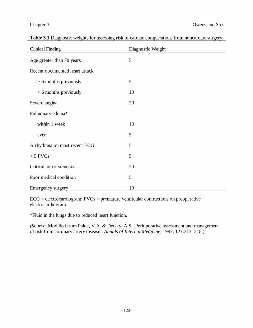
Chapter 3 Owens and Sox
-123-123
Table 3.1 Diagnostic weights for assessing risk of cardiac complications from noncardiac surgery.
Clinical Finding Diagnostic Weight
Age greater than 70 years 5
Recent documented heart attack
> 6 months previously
< 6 months previously
5
10
Severe angina 20
Pulmonary edema*
within 1 week
ever
10
5
Arrhythmia on most recent ECG 5
> 5 PVCs 5
Critical aortic stenosis 20
Poor medical condition 5
Emergency surgery 10
ECG = electrocardiogram; PVCs = premature ventricular contractions on preoperativeelectrocardiogram.
*Fluid in the lungs due to reduced heart function.
(Source: Modified from Palda, V.A. & Detsky, A.S. Perioperative assessment and managementof risk from coronary artery disease. Annals of Internal Medicine, 1997; 127:313–318.)
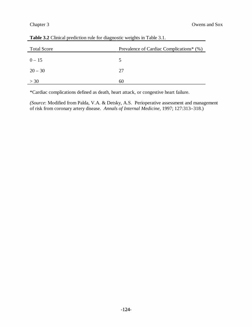
Chapter 3 Owens and Sox
-124-124
Table 3.2 Clinical prediction rule for diagnostic weights in Table 3.1.
Total Score Prevalence of Cardiac Complications* (%)
0 – 15 5
20 – 30 27
> 30 60
*Cardiac complications defined as death, heart attack, or congestive heart failure.
(Source: Modified from Palda, V.A. & Detsky, A.S. Perioperative assessment and managementof risk from coronary artery disease. Annals of Internal Medicine, 1997; 127:313–318.)
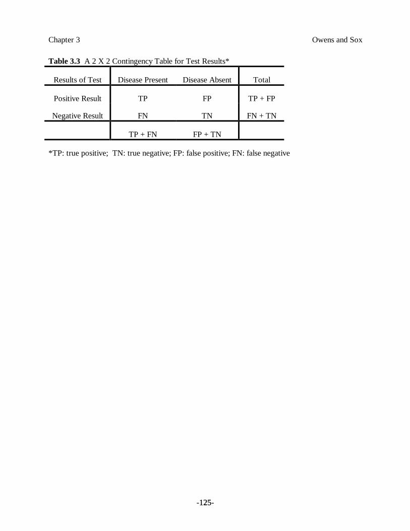
Chapter 3 Owens and Sox
-125-125
Table 3.3 A 2 X 2 Contingency Table for Test Results*
Results of Test Disease Present Disease Absent Total
Positive Result TP FP TP + FP
Negative Result FN TN FN + TN
TP + FN FP + TN
*TP: true positive; TN: true negative; FP: false positive; FN: false negative
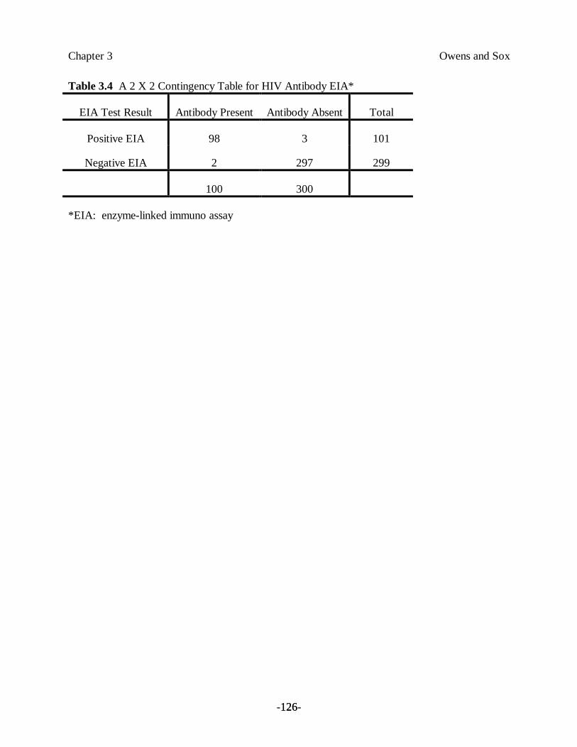
Chapter 3 Owens and Sox
-126-126
Table 3.4 A 2 X 2 Contingency Table for HIV Antibody EIA*
EIA Test Result Antibody Present Antibody Absent Total
Positive EIA 98 3 101
Negative EIA 2 297 299
100 300
*EIA: enzyme-linked immuno assay
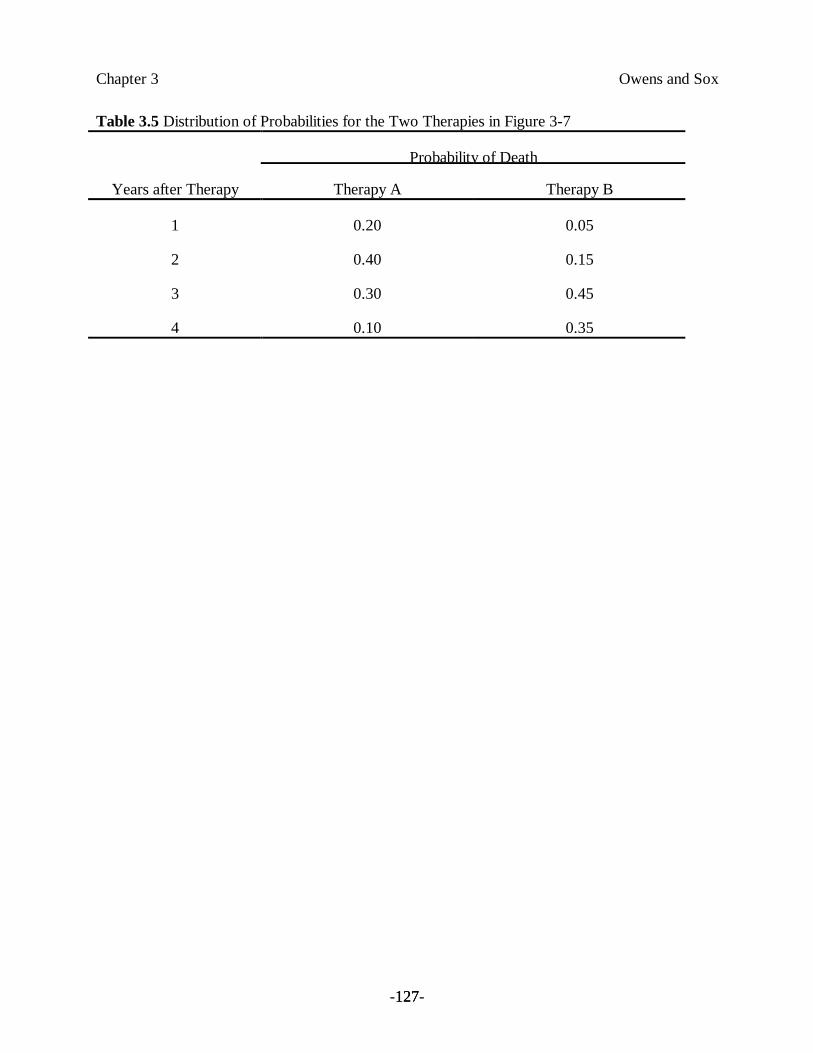
Chapter 3 Owens and Sox
-127-127
Table 3.5 Distribution of Probabilities for the Two Therapies in Figure 3-7
Probability of Death
Years after Therapy Therapy A Therapy B
1 0.20 0.05
2 0.40 0.15
3 0.30 0.45
4 0.10 0.35
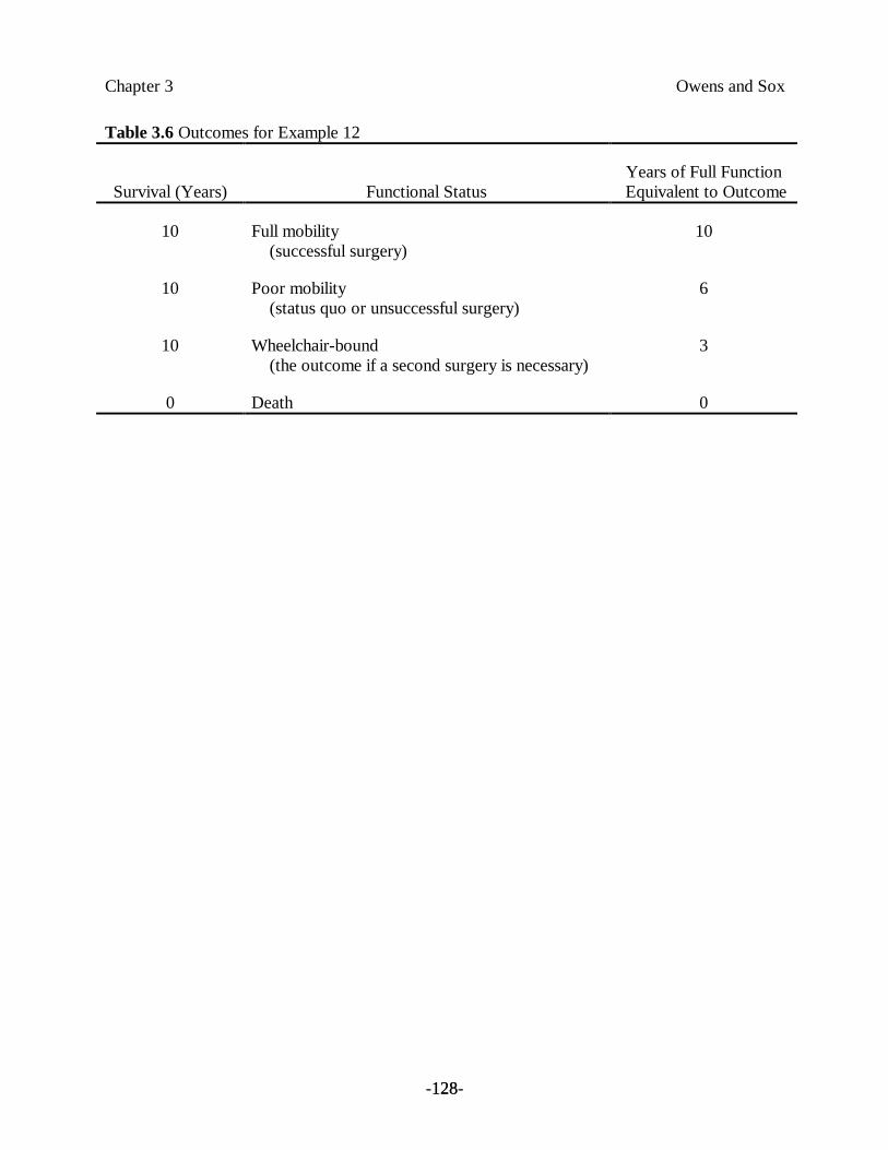
Chapter 3 Owens and Sox
-128-128
Table 3.6 Outcomes for Example 12
Survival (Years) Functional StatusYears of Full Function
Equivalent to Outcome
10 Full mobility (successful surgery)
10
10 Poor mobility (status quo or unsuccessful surgery)
6
10 Wheelchair-bound (the outcome if a second surgery is necessary)
3
0 Death 0

Chapter 3 Owens and Sox
-129-129
Table 3.7 Transition probabilities for the Markov model in Figure 3.13.
Health-State Transition Annual Probability
Well to Well 0.9
Well to Cancer 0.06
Well to Death 0.04
Cancer to Well 0.0
Cancer to Cancer 0.4
Cancer to Death 0.6
Death to Well 0.0
Death to Cancer 0.0
Death to Death 1.0
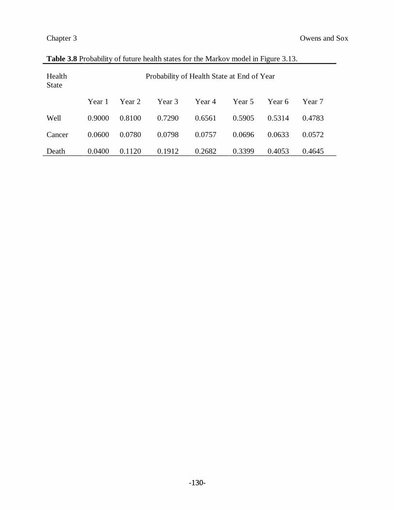
Chapter 3 Owens and Sox
-130-130
Table 3.8 Probability of future health states for the Markov model in Figure 3.13.
HealthState
Probability of Health State at End of Year
Year 1 Year 2 Year 3 Year 4 Year 5 Year 6 Year 7
Well 0.9000 0.8100 0.7290 0.6561 0.5905 0.5314 0.4783
Cancer 0.0600 0.0780 0.0798 0.0757 0.0696 0.0633 0.0572
Death 0.0400 0.1120 0.1912 0.2682 0.3399 0.4053 0.4645
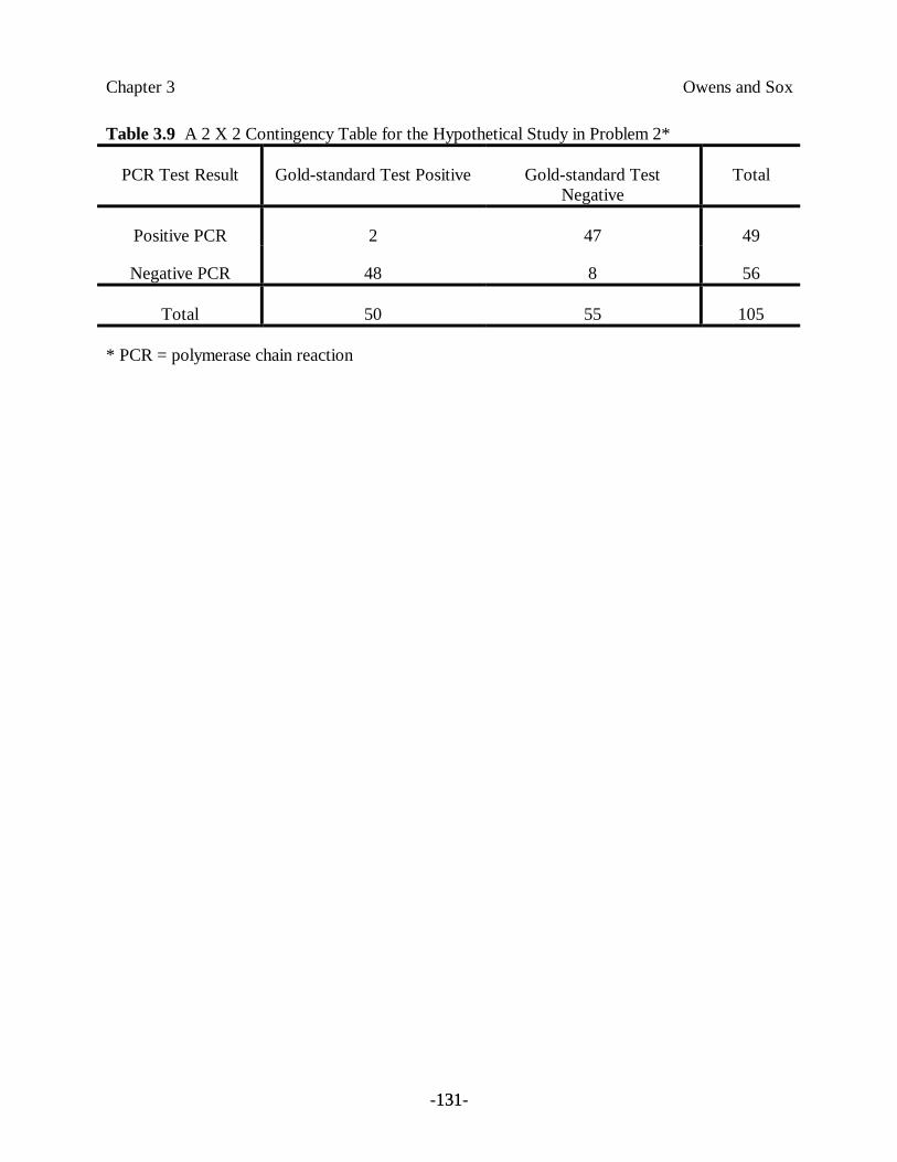
Chapter 3 Owens and Sox
-131-131
Table 3.9 A 2 X 2 Contingency Table for the Hypothetical Study in Problem 2*
PCR Test Result Gold-standard Test Positive Gold-standard TestNegative
Total
Positive PCR 2 47 49
Negative PCR 48 8 56
Total 50 55 105
* PCR = polymerase chain reaction
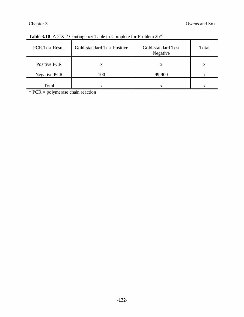
Chapter 3 Owens and Sox
-132-132
Table 3.10 A 2 X 2 Contingency Table to Complete for Problem 2b*
PCR Test Result Gold-standard Test Positive Gold-standard TestNegative
Total
Positive PCR x x x
Negative PCR 100 99,900 x
Total x x x* PCR = polymerase chain reaction
Chapter 3 Owens and Sox
-133-133
Legends to Figures
Figure 3.1 Probability and descriptive terms. Different physicians attach different meanings to thesame terms. The bars show the wide variation in point probabilities assigned by individualphysicians and other health-care workers when they were asked to interpret these terms.(Reprinted, by permission, from Bryant, G.D. and Norman, G.R. Expressions of probability:Words and numbers. New England Journal of Medicine, 302:411, 1980.)
Figure 3.2 The effect of test results on the probability of disease. (a) A positive test result oftenincreases the probability of disease. (b) Test 2 reduces uncertainty about presence of disease(increases the probability of disease) more than test 1 does.
Figure 3.3 Distribution of test results in healthy and diseased individuals. Varying the cutoffbetween “normal” and “abnormal” across the continuous range of possible values will change therelative proportions of false positives and false negatives for the two populations.
Figure 3.4 Receiver operating characteristic (ROC) curves for two hypothetical tests. Test B ismore discriminative than test A is because its curve is higher (for example, the false-positive ratefor test B is lower than the false-positive rate for test A is at any value of true-positive rate). Themore discriminative test may not always be preferred in clinical practice, however (see text).
Figure 3.5 Relationship between pretest probability and posttest probability of disease. Thedotted line corresponds to a test that has no effect on the probability of disease. Sensitivity andspecificity of the test were assumed to be 0.90 for the two examples. (a) The posttest probabilityof disease corresponding to a positive test result (solid curve) was calculated with Bayes’ theoremfor all values of pretest probability. (b) The posttest probability of disease corresponding to anegative test result (solid curve) was calculated with Bayes’ theorem for all values of pretestprobability. (Source: Adapted from Sox, H.C. Probability theory in the use of diagnostic tests:Application to critical study of the literature. In Sox, H.C. (ed), Common Diagnostic Tests: Useand Interpretation. Philadelphia: American College of Physicians, 1987, p. 1–17. Reproducedwith permission from the American College of Physicians – American Society of InternalMedicine.)
Figure 3.6 Effect of test sensitivity and specificity on posttest probability. The curves are similarto those shown in Figure 3.5, except that the calculations have been repeated for several values ofthe sensitivity (TPR, true-positive rate) and specificity (TNR, true-negative rate) of the test. (a)The sensitivity of the test was assumed to be 0.90, and the calculations were repeated for severalvalues of test specificity. (b) The specificity of the test was assumed to be 0.90, and thecalculations were repeated for several values of the sensitivity of the test. In both panels, the topfamily of curves corresponds to positive test results, and the bottom family of curves correspondsto negative test results. (Source: Adapted from Sox, H.C. Probability theory in the use ofdiagnostic tests: Application to critical study of the literature. In Sox, H.C. (ed), CommonDiagnostic Tests: Use and Interpretation. Philadelphia: American College of Physicians, 1987, p.1–17. Reproduced with permission from the American College of Physicians – American Societyof Internal Medicine.)
Chapter 3 Owens and Sox
-134-134
Figure 3.7 Survival after therapy for a fatal disease. Two therapies are available; the results ofeither are unpredictable.
Figure 3.8 A chance-node representation of survival after the two therapies in Figure 3.7. Theprobabilities times the corresponding years of survival are summed to obtain the total expectedsurvival.
Figure 3.9 Decision tree for knee-replacement surgery. The box represents the decision node(whether to have surgery). The circles represent chance nodes.
Figure 3.10 Decision tree for knee-replacement surgery. Probabilities have been assigned to eachbranch of each chance node. The patient’s valuations of outcomes (measured in years of perfectmobility) are assigned to the tips of each branch of the tree.
Figure 3.11 Sensitivity analysis of the effect of operative mortality on length of healthy life(Example 12). As the probability of operative death increases, the relative values of surgeryversus no surgery change. The point at which the two lines cross represents the probability ofoperative death at which no surgery becomes preferable. The solid line represents the preferredoption at a given probability.
Figure 3.12 Sensitivity analysis of the effect of a successful operative result on length of healthylife (Example 12). As the probability of a successful surgical result increases, the relative valuesof surgery versus no surgery change. The point at which the two lines cross represents theprobability of a successful result at which surgery becomes preferable. The solid line representsthe preferred option at a given probability.
Figure 3.13 A simple Markov model. The states of health that a person can experience areindicated by the circles. Arrows represent allowed transitions between health states.
Figure 3.14 Depiction of the treatment-threshold probability. At probabilities of disease that areless than the treatment-threshold probability, the preferred action is to withhold therapy. Atprobabilities of disease that are greater than the treatment-threshold probability, the preferredaction is to treat.
Figure 3.15 Decision tree with which to calculate the treatment-threshold probability of disease.By setting the utilities of the treat and do not treat choices to be equal, we can compute theprobability at which the physician and patient should be indifferent to the choice. Recall thatp[− D] = 1 − p[D].
Figure 3.16 An influence diagram (right)[lower? Depends on placement on the page] anddecision tree (left)[upper? Depends on placement on the page] that represent the decisions to testfor and to treat HIV infection. The structural asymmetry of the alternatives is explicit in thedecision tree. The influence diagram highlights probabilistic relationships. HIV = humanimmunodeficiency virus; HIV+ = HIV-infected; HIV– = not infected with HIV; QALE = quality-adjusted life expectancy; PCR = polymerase chain reaction. Test results are shown in quotationmarks (“HIV+”), whereas the true disease state is shown without quotation marks (HIV+).
Chapter 3 Owens and Sox
-135-135
(Source: Owens D.K., Shachter R.D., Nease R.F. Representation and analysis of medicaldecision problems with influence diagrams. Medical Decision Making, 17(3): 241–262, 1997.Reproduced with permission.)
Figure 3.17 The influence diagram from Figure 3.16, with the probability and value tablesassociated with the nodes. The information in these tables is the same as that associated with thebranches and endpoints of the decision tree in Figure 3.16. HIV = human immunodeficiency virus;HIV+ = HIV-infected; HIV– = not infected with HIV; QALE = quality-adjusted life expectancy;PCR = polymerase chain reaction; NA = not applicable; Tx+ = treated; TX– = not treated. Testresults are shown in quotation marks (“HIV+”) and the true disease state is shown withoutquotation marks (HIV+). (Source: Owens, D.K., Shachter, R.D., Nease, R.F. Representationand analysis of medical decision problems with influence diagrams. Medical Decision Making,1997; 17: 241–262. Reproduced with permission.)
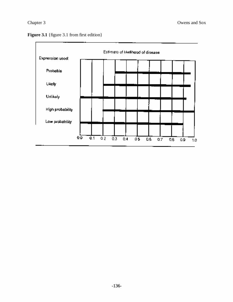
Chapter 3 Owens and Sox
-136-136
Figure 3.1 {figure 3.1 from first edition}
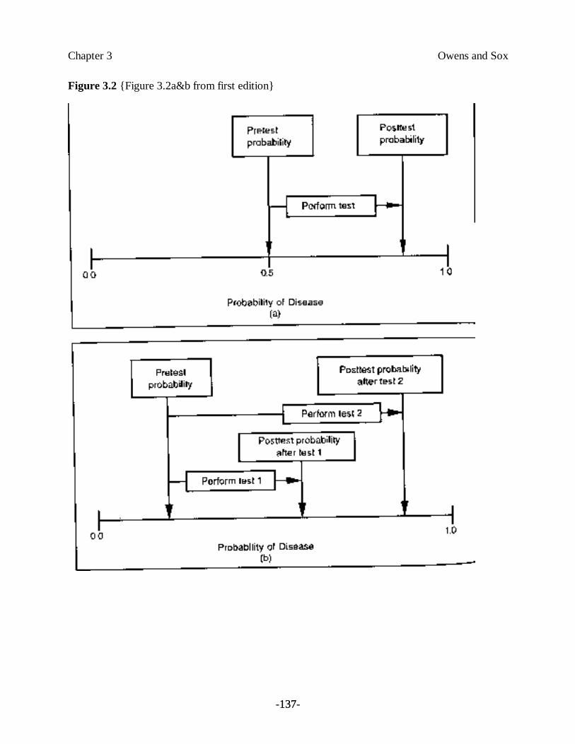
Chapter 3 Owens and Sox
-137-137
Figure 3.2 {Figure 3.2a&b from first edition}
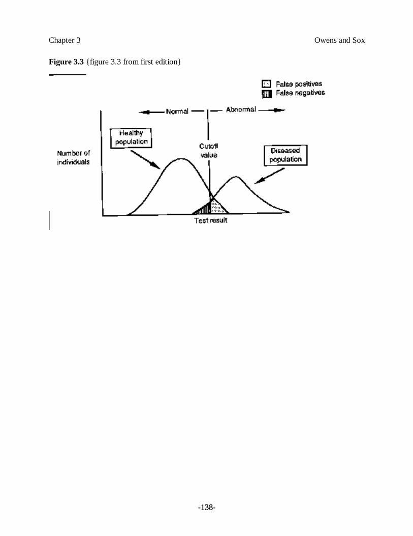
Chapter 3 Owens and Sox
-138-138
Figure 3.3 {figure 3.3 from first edition}
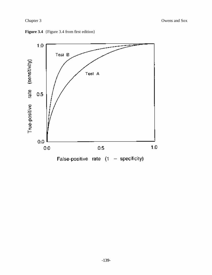
Chapter 3 Owens and Sox
-139-139
Figure 3.4 {Figure 3.4 from first edition}
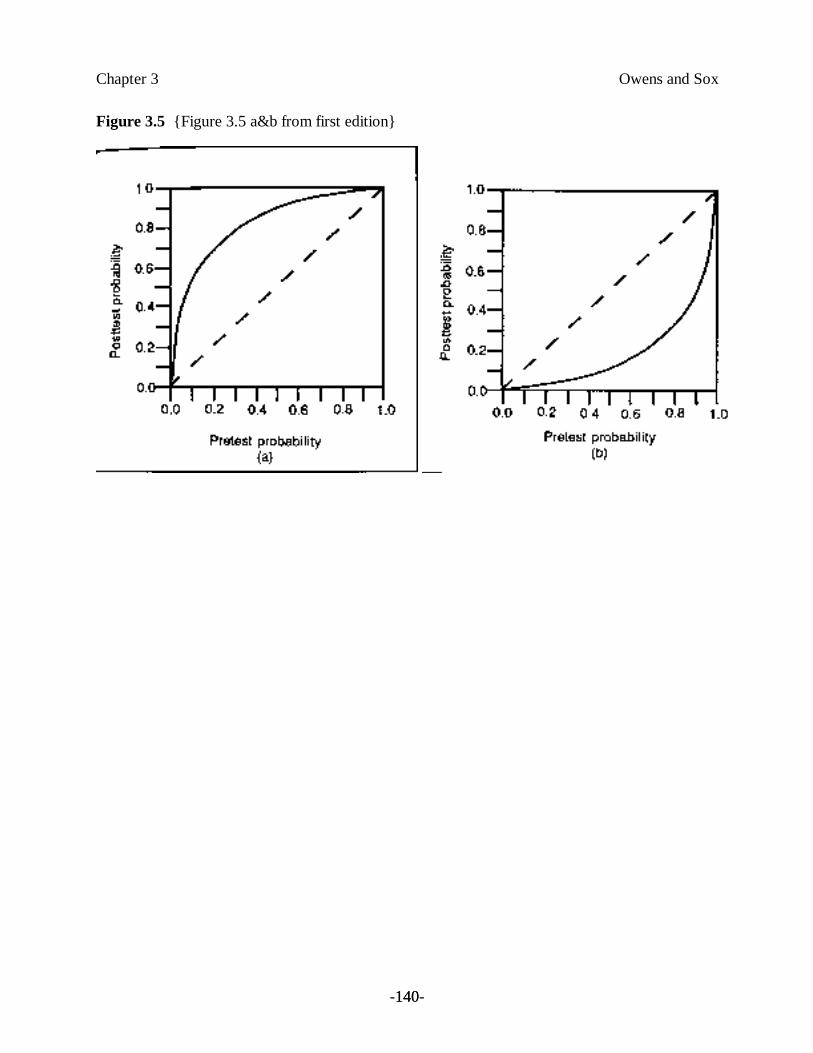
Chapter 3 Owens and Sox
-140-140
Figure 3.5 {Figure 3.5 a&b from first edition}
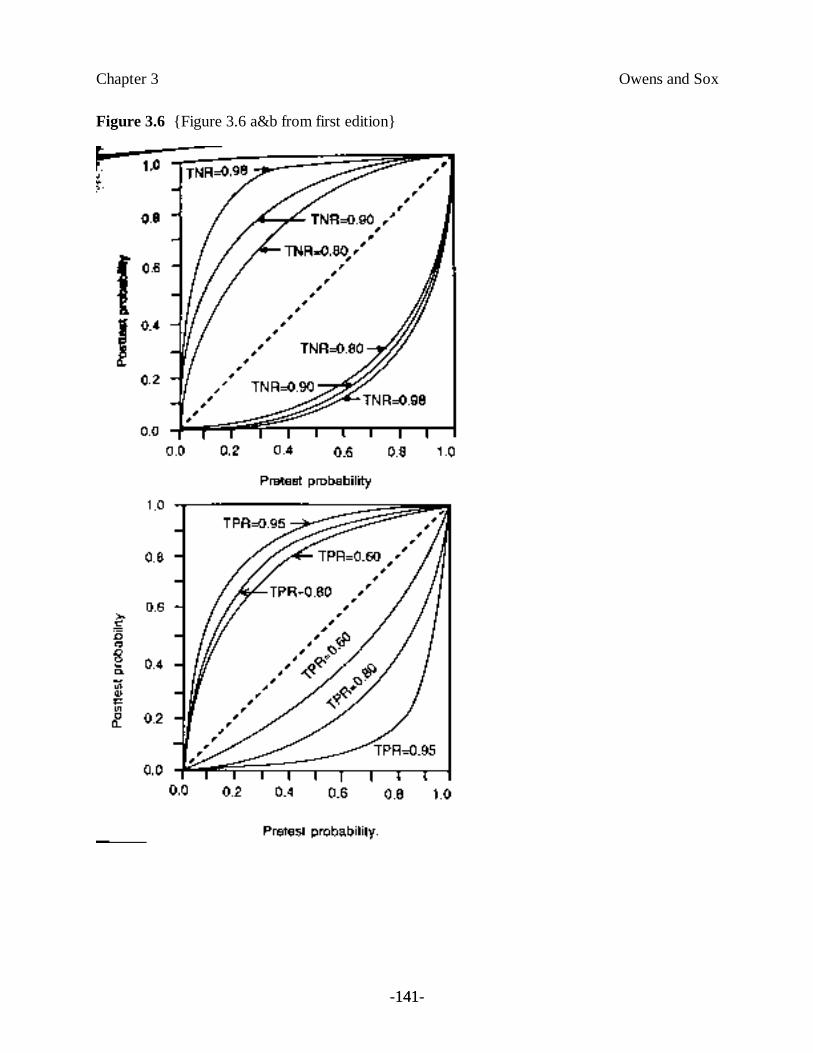
Chapter 3 Owens and Sox
-141-141
Figure 3.6 {Figure 3.6 a&b from first edition}
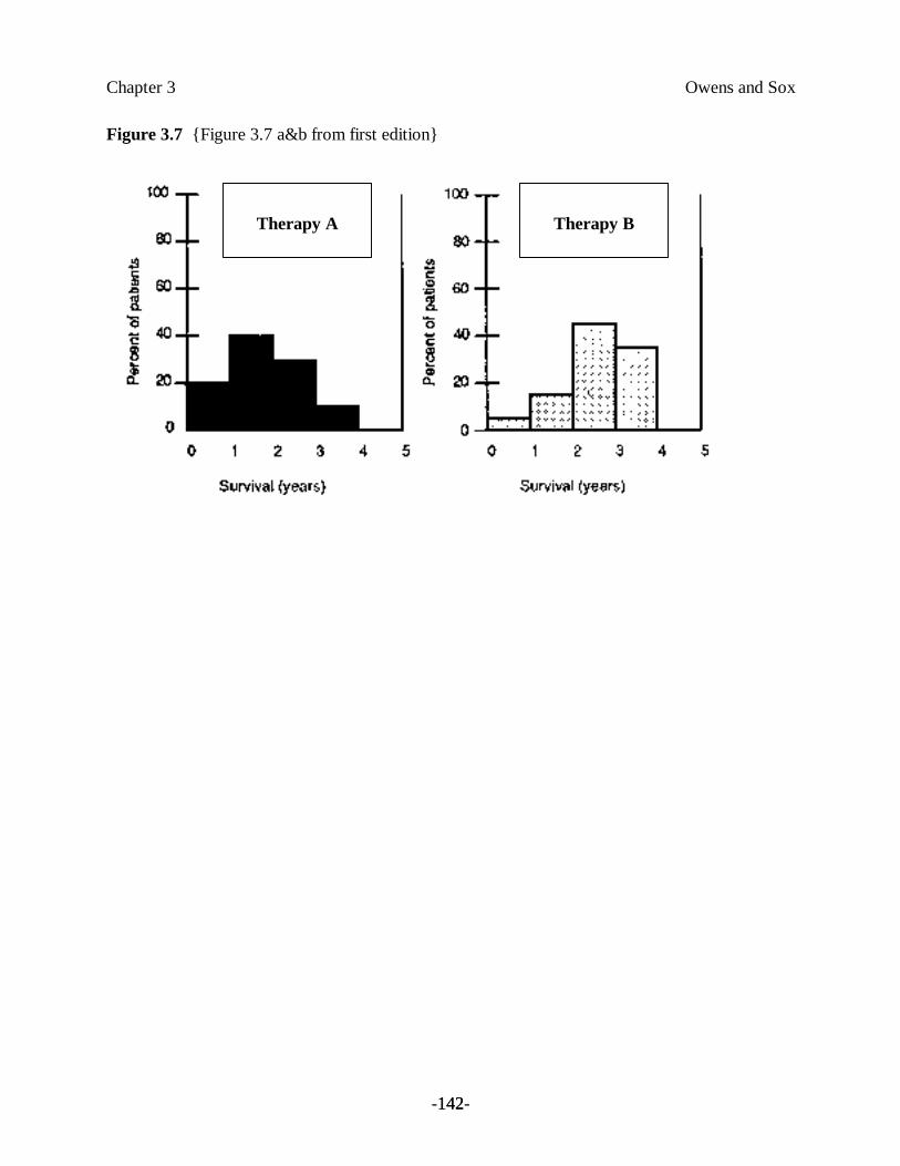
Chapter 3 Owens and Sox
-142-142
Figure 3.7 {Figure 3.7 a&b from first edition}
Therapy A Therapy B

Chapter 3 Owens and Sox
-143-143
Figure 3.8 {Figure 3.8 from first edition}
Therapy A Therapy B
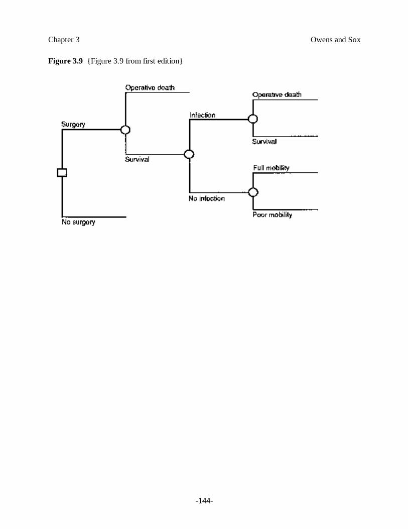
Chapter 3 Owens and Sox
-144-144
Figure 3.9 {Figure 3.9 from first edition}
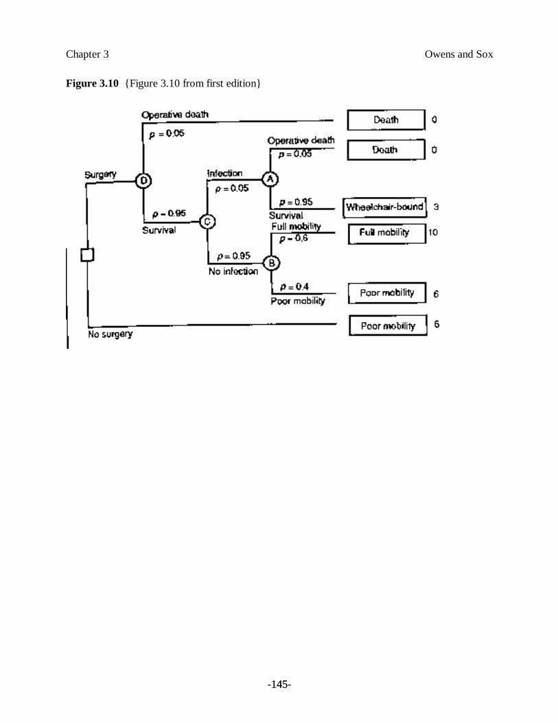
Chapter 3 Owens and Sox
-145-145
Figure 3.10 {Figure 3.10 from first edition}
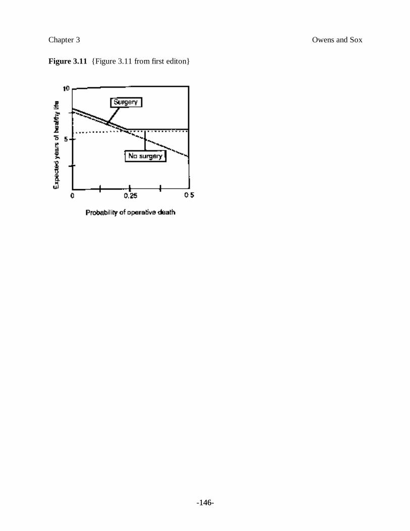
Chapter 3 Owens and Sox
-146-146
Figure 3.11 {Figure 3.11 from first editon}
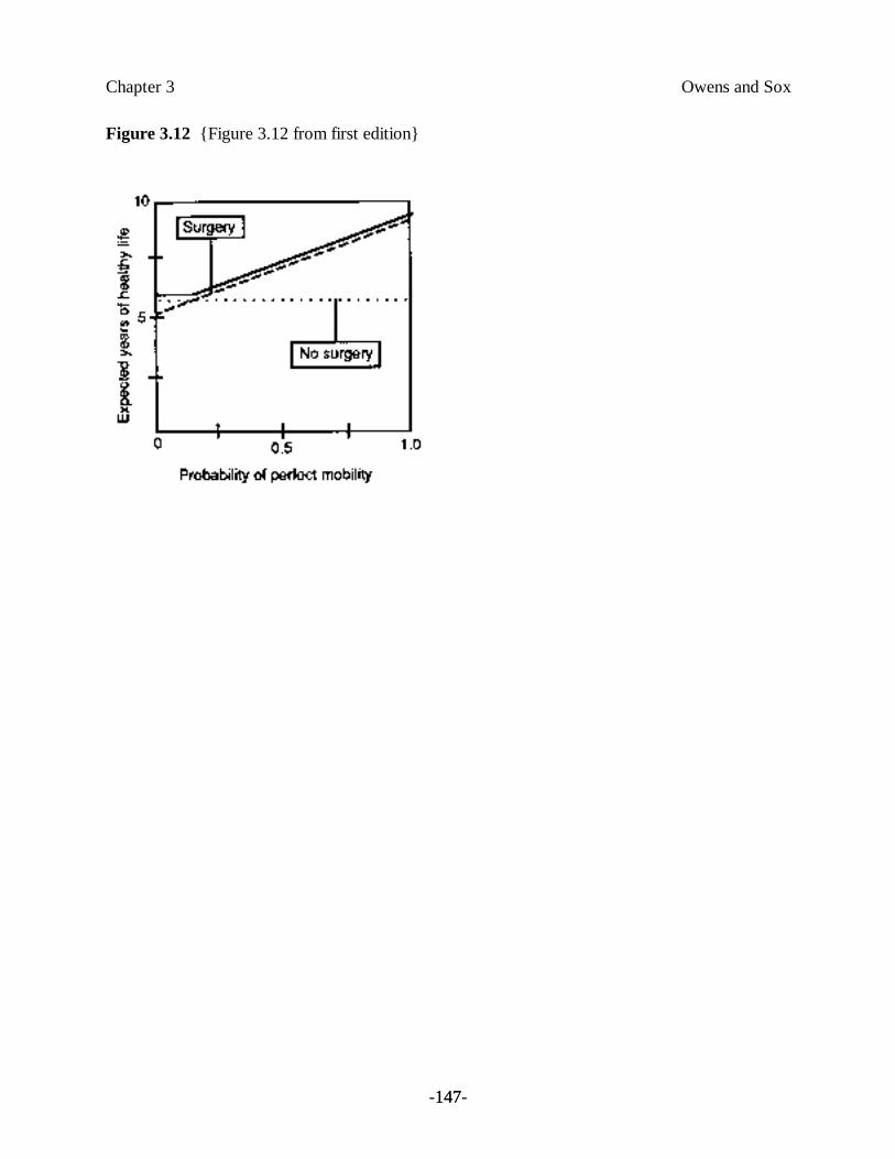
Chapter 3 Owens and Sox
-147-147
Figure 3.12 {Figure 3.12 from first edition}
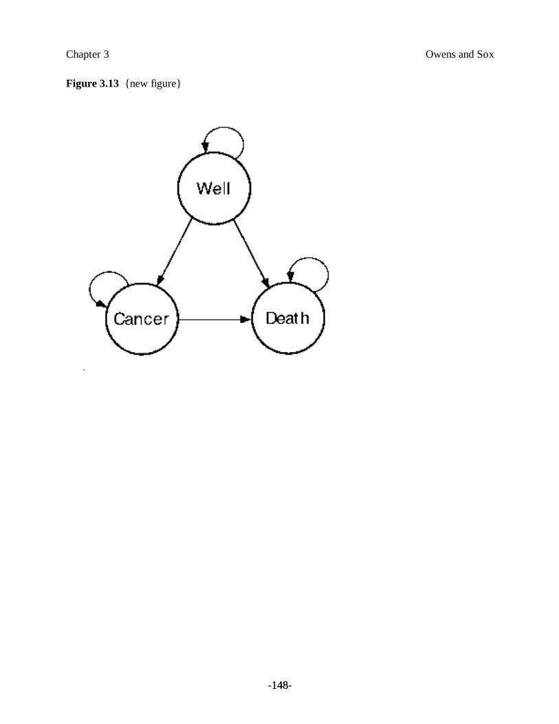
Chapter 3 Owens and Sox
-148-148
Figure 3.13 {new figure}
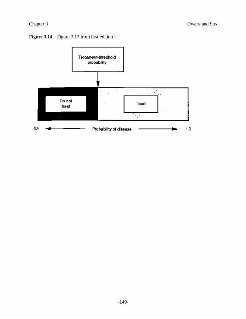
Chapter 3 Owens and Sox
-149-149
Figure 3.14 {Figure 3.13 from first edition}

Chapter 3 Owens and Sox
-150-150
Figure 3.15 {Figure 3.14 from first edition}
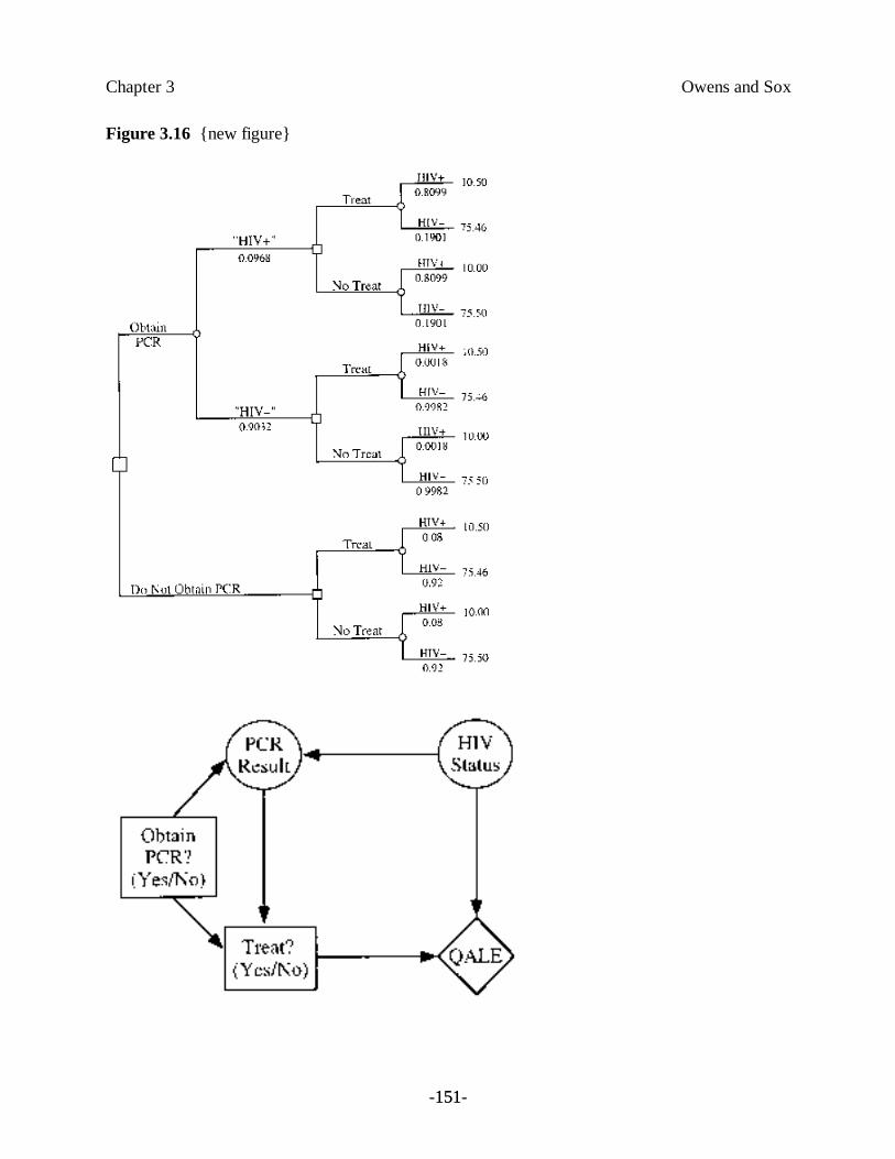
Chapter 3 Owens and Sox
-151-151
Figure 3.16 {new figure}
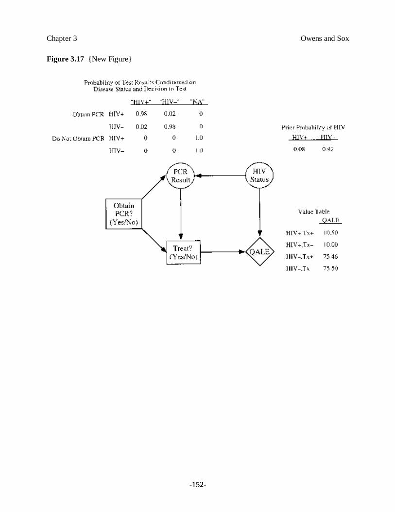
Chapter 3 Owens and Sox
-152-152
Figure 3.17 {New Figure}