chapter 3 kinetic monte carlo modelinginfohouse.p2ric.org/ref/31/30084/ch3.pdf · chapter 3 kinetic...
TRANSCRIPT
22
Chapter 3
Kinetic Monte Carlo Modeling
3.1 Introduction
The “Monte Carlo method” has its name from the use of “random numbers” to
simulate statistical fluctuations in order to numerically generate probability distributions
[64]. It is generally believed that the widespread use of Monte Carlo concept began with
the Metropolis algorithm in the calculation for a rigid-sphere system [42]. This technique
can be readily used to study equilibrium properties of a system of atoms. Since the kinetic
path of evolution is physically meaningless in this scheme, it is not suitable for treating
atomic assembly process in vapor deposition.
This chapter gives a detailed account of the kinetic Monte Carlo method which is
suitable for simulating kinetic evolution process. The n-fold way algorithm [65] is first
introduced which is believed to be the earliest form of the current kMC concept. A formal
kMC procedure specifically formulated for simulating thin film growth in this thesis is
next described. As a critical part of the kMC method, the activation barrier calculation
through interatomic force law derived from the embedded atom method (EAM) is then
followed. Finally, the basic principles of molecular dynamics method is explained. Molec-
ular dynamics calculations provide a viable means to simulate the initial interactions of an
incident atom with a growing film and enable the kMC to approximate the effects of
kinetic energy through a kMC-MD coupling procedure introduced in chapter seven.

Kinetic Monte Carlo Modeling 23
3.2 n-fold way algorithm
The term “kinetic Monte Carlo” was initiated by Horia Metiu, Yan-Ten Lu and
Zhenyu Zhang in a 1992 Science paper titled “Epitaxial Growth and the Art of Computer
Simulations” [51]. The paper first pointed out the demands on atomic level control of
modern electronic and photonic devices and the importance of in situ STM observations
of small atomic “clusters” to a theorist who wants to understand growth and segregation; it
then elaborated upon the usefulness of kMC simulations in reproducing these experimen-
tal observations. The basic feature of their model was to move atoms site-to-site on a
square lattice terrace. They postulated rates for all of the elementary processes involved,
such as the site-to-site jumps, the jumps to leave or join a step or an existing adsorbate
cluster, and so forth. The atoms were deposited on the surface and moved from site to site
with a frequency proportional to the rate of the respective move: if the rate constant of the
i-th kinetic process was ki, the largest rate was chosen as a reference and denoted kr. The
probability Pi = ki/kr was then used in a Monte Carlo program as the probability that the
atom performed a jump i. The work used Voter’s transition state theory [66] to monitor the
simulation time. The overall scheme was close to what is used now and the essence
through the references can be traced to Bortz, Kalow, and Lebowitz’s n-fold way algo-
rithm [65, 67, 68] which appeared in 1975.
The n-fold way idea was created to replace the standard Monte Carlo algorithm in
generating new configurations in simulating Ising spin systems. In or near the equilibrium
state, the standard MC scheme using a Boltzmann kinetic factor, exp(-∆E/kT), (where ∆E
is the system energy change, k is the Boltzmann constant and T the absolute temperature)
becomes very inefficient since the Boltzmann factor is usually very small in comparison
with a random number over the interval [0, 1] [65]. On the other hand, the n-fold way
chooses a spin site from the entire ensemble based upon its probability of flipping. Once a
site was selected, the flipping was guaranteed and could be immediately performed. The
n-fold way also provided a new simulation time concept. At each flip, the time was incre-

Kinetic Monte Carlo Modeling 24
mented by a stochastic variable, ∆t, whose expectation value is proportional to
(where Q10 is the number of spins times the average probability that an attempt will pro-
duce a flip for a given configuration). Mathematically, , where R is a
random fraction and τ a system dependent time. This choice reflects properly the distribu-
tion of time intervals between flips for a reasonable physical model. The cumulative time
thus summed is approximately proportional to real time. The n-fold way reduced compu-
tation time by an order of magnitude or more for many applications [65]. A similar con-
cept was used in Voter’s 1987 transition state theory [66].
3.3 Kinetic Monte Carlo Method
The vapor deposition process consists of several distinct steps, creation of the
vapor, the transport of species to the substrate, interaction of the incident atoms with the
growing film, assembly of the adatoms on the substrate through diffusion process leading
to either the incorporation of the adatom or its evaporation. To simulate the vapor growth
process, all of the process should be incorporated. The most important step, however, is to
correctly simulate the diffusion. Although diffusion may not be important at low tempera-
ture or very high deposition rate and can be approximated accordingly using the HBC
model [46], in most practical situations deposition is conducted under conditions where
atomic diffusion occurs simultaneously with deposition. This thermal diffusion must
therefore be taken into account. The methodology should also address the many diffu-
sional pathways available. It should also connect with the temperature and deposition rate
since these control the available time for surface diffusional processes before the surface
becomes covered by a new atom layer.
If Boltzmann statistics are assumed to govern the diffusional processes, the proba-
bility per unit time for a possible jump, i, to take place is given by:
Q101–
∆t τ Q10⁄( ) Rln–=

Kinetic Monte Carlo Modeling 25
3-1
where ν0 is the effective vibration frequency (taken to be 5×10¹²/s for all the cases in this
work), Ei is the activation energy for the i-th type of jump, k is Boltzmann’s constant and T
is the absolute temperature.
The reciprocal of an atomic jump probability per unit time is a residence time for
an atom that moves by that specific type of jump. Since the jump probabilities of all the
different types of jumps are independent, the overall probability per unit time for the sys-
tem to change its state by any type of jump step is just the sum of all the possible specific
jump type probabilities, and so the residence time for the system in a specific configura-
tion is the reciprocal of this overall jump probability. The next diffusional step is deter-
mined by randomly choosing from among all the possible jumps weighted by their relative
probability of occurrence. By following the ensuing discrete jump path for the system,
accumulating the residence time of the system along the path, and linking this history to
the adatom arrival interval (or the deposition rate), the diffusion process can be realisti-
cally simulated.
The calculation begins by determining a time interval between adatom arrivals
based on the deposition rate. The average time interval between the arrival of two atoms in
a 2D lattice model is
3-2
where R is the deposition rate, a is the nearest neighbor distance and n is the number of
atoms comprising a monolayer in a close-packed 2D lattice. Clearly, the higher the deposi-
tion rate, the smaller the time interval between two consecutive deposition events in the
pi ν0Ei
kT------–
exp=
∆t 3a2nR----------=

Kinetic Monte Carlo Modeling 26
model. Time periods are then related to the diffusion process through a net (system) resi-
dence time, tn, given by:
3-3
where N is the number of different types of jumps (i.e. different diffusion pathways). In
this model, a single jump is allowed only to vacant nearest-neighbor sites or over a ledge
at the surface, i.e. a Schwoebel jump [50]. The two time definitions (Eqns. 3-2 and 3-3)
are then linked for the simulation.
An atom can then be dropped from a random position above the surface. It travels
to the surface in a straight line and impacts the substrate at an angle θ to the normal. It is
then instantly relaxed to the closest available lattice site. The set of atoms in the simulation
system can then be monitored for diffusional modification prior to the arrival of the next
atom, i.e. in the time ∆t. If the system has a net jump probability greater than 1 in the ∆t
time period, a jump is made and a time equal to the net residence time (calculated using
Eqn. 3-3) is subtracted from ∆t so that there is less time remaining for further jumps in the
allotted time period. This process is iterated until the probability of making any jump in
the remaining time is less than one. Whether or not any jump is made in this time period
can then be determined by random choice based on the remaining time and the net time for
that particular state of the system. Whenever a jump is to be made, the specific one is
determined by random choice based on the relative probabilities of all potential jumps.
When the remaining time reaches zero, the clock is turned ahead by ∆t and another atom is
then deposited. An implementation algorithm of this thermal diffusion simulation is
described in next chapter.
tn pi
i 1=
N
∑ 1–
=
Kinetic Monte Carlo Modeling 27
3.4 Interatomic potentials
The concept of kMC simulation provides a powerful tool in the study of atom by
atom assembly process of vapor deposition which is not accessible in experiment except
for only a few techniques such as STM [69]. As a result, physical properties for most of
the individual surface motions are extremely difficult to obtain under real observations.
For example, the probability for an atomic jump occurrence depends upon a jump attempt
rate (here assumed to be the maximum lattice vibration frequency) and the activation bar-
rier for the jump. Very little experimental data about the magnitude of the barrier height
exists. Thus alternatives must be sought to quantify them. The ab-initio methods solving
the many-electron Schrödinger equation would be desirable [70], but they are computa-
tionally expensive. Even with approximations to this scheme, such as the local-density
approximation (LDA), and with recent impressive advances in computers and algorithms,
these traditional band-structure calculations are impractical for systems with very low
symmetry, such as grain boundaries [71].
An alternative approach is through the analysis of interatomic force laws which are
often empirically derived by fitting coefficients in physical expressions to experimental
quantities. The traditional two-body potentials such as Lennard-Jones potential, while
yielding the total energy directly, require the use of an accompanying volume-dependent
energy to correctly describe the elastic properties of a metal [72]. However, this volume
becomes ambiguous to define in calculations involving surfaces [72], which would inevi-
tably lead to inaccurate estimates of the activation barriers for atom migration on a sur-
face.
A major development in addressing multi-body effect came in 1983 when Daw
and Baskes proposed the embedded atom method (EAM) [73, 74]. The key assumption in
the EAM procedure is that all atoms are viewed as being embedded in the host consisting
of all other atoms. The embedding energy is electron-density dependent. Because the elec-

Kinetic Monte Carlo Modeling 28
tron density is always definable, the problem of the ambiguity of defining the volume is
circumvented. With these advantages, the EAM has attained a considerable success in
problems, often intractable with pair potentials alone, covering a broad range of metals,
impurities, alloys and surface properties.
In the following sections, Johnson’s format of the EAM potential [76, 77, 80] is
introduced, followed by the fitting procedure needed to develop a specific nickel and cop-
per EAM potential for use in this thesis along with the molecular statics method needed to
deduce the activation energy parameters.
3.4.1 Embedded atom method potentials
In EAM, the energy of the metal is viewed as the energy obtained by embedding
an atom into the local electron density provided by the remaining atoms of the system. In
addition, there is a two-body central interaction. The basic equations are of the form:
i = 1, 2,..., N. 3-4
where i, j = 1,2,..., N 3-5
and i, j = 1, 2,..., N 3-6
Etot is the total internal energy of an assembly of atoms, Ei is the internal energy associ-
ated with atom i, ρi is the total electron density at atom i due to the rest of the atoms in the
system, Fi(ρi) is the energy to embed atom i into the electron density ρi, φij(rij) is the two-
body central potential between atom i and atom j separated by a distance rij, and fj(rij) is
the contribution to the electron density at atom i due to atom j at a distance rij from atom i.
Etot Ei
i
∑=
Ei Fi ρi( ) 12--- φij rij( )
i j≠∑+=
ρi fj rij( )i j≠∑=

Kinetic Monte Carlo Modeling 29
Generally, the first term in Eqn. 3-5, the embedding energy, is dominant in provid-
ing atomic cohesion. Because the electron density comes from all of the neighboring
atoms, the atom-host interaction is described in a way that is inherently more complex
than the two-bond model. In this way, the embedding function incorporates some impor-
tant many-atom interactions and demonstrates how bonding is affected by coordination.
This naturally leads to an understanding of the difference between bulk and surface bonds,
an essential feature in thin film growth process. However, it was found [74] that, for the
special case when F(ρ) is a linear function, the entire scheme is equivalent to the use of a
different pair potential. In other words, must be a non-zero number to ensure the multi-
body interaction in the EAM scheme.
Actually, the first-principles calculations by Daw [75] did reveal that the embed-
ding function should have a positive curvature for the background electron densities found
in metals, that is . On the other hand, the EAM model’s invariation to the linear
transformation (i.e. adding a linear contribution to the embedding function can be exactly
compensated by a change in the pair interaction) makes it possible to construct an effec-
tive two-body potential. For example, one can have an embedding function with zero
slope at the equilibrium electron density for a perfect lattice configuration: .
The change from the perfect crystal energy is then dominated by the effective two-body
potential for any atomic configuration in which the electron density at atom sites is not
significantly altered. Since the electron density at an atom site is a superposition of the
contribution from all neighboring atoms, its change is commonly small in defect configu-
rations in tight-packed metals. Any EAM model can be so transformed and such a trans-
formed model is called the normalized form of EAM [76, 77]. However, the present EAM
form will not work as well for systems where directional bonding is important, such as
semiconductors and elements from the middle of the transition series [78].
F″
d2F
dρ2--------- 0>
dFdρ-------
e0=

Kinetic Monte Carlo Modeling 30
3.4.2 EAM potential fitting
To apply this method, the embedding energies, pair interaction, and electron densi-
ties expressed in Eqns. 3-4, 3-5 and 3-6 must be given. Daw has taken electron densities
from Hartree-Fock calculations and calculated approximate values of the embedding ener-
gies and pair interactions from the formal definitions of these quantities in the density-
functional framework [75]. Since these values only gave qualitatively correct predictions
of the material properties, it is necessary to determine these functions empirically to obtain
an accurate description.
Since the purpose behind two-dimensional atomistic calculations for vapor deposi-
tion (most of work in this thesis) is to obtain guidance in understanding the mechanisms
and critical factors involved in the process and to seek trends and gain insight, there is lit-
tle need to fit the atomistic model precisely to a specific material and the model should be
as computationally efficient as possible [81]. However, for comparative studies a consis-
tent model which gives a sense of the scaling between materials and the effect of alloying
should be used. A nearest-neighbor embedded-atom method model fits these qualifica-
tions for metals [81].
A common practice in applying the normalized EAM is to first choose the specific
functional form for φ(r) and f(r), fit the model parameters in φ(r) and f(r) to experimental
data of lattice parameter a or the atomic volume Ω (Ω = a3/4 for fcc metals), the cohesive
energy Ec, the approximate vacancy formation energy , the bulk modulus Bv and Voigt
average shear modulus Gv. The bulk modulus represents the resistance to volume change,
while the Voigt average shear modulus represents the resistance to shear deformation.
For the embedding function, Foiles’ scheme via the equation of state of the pure
metals [79] was often used to obtain F(ρ) in the early days. Now an analytic form pro-
posed by Johnson and Oh [76] is frequently applied for the embedded function:
Ef
Kinetic Monte Carlo Modeling 31
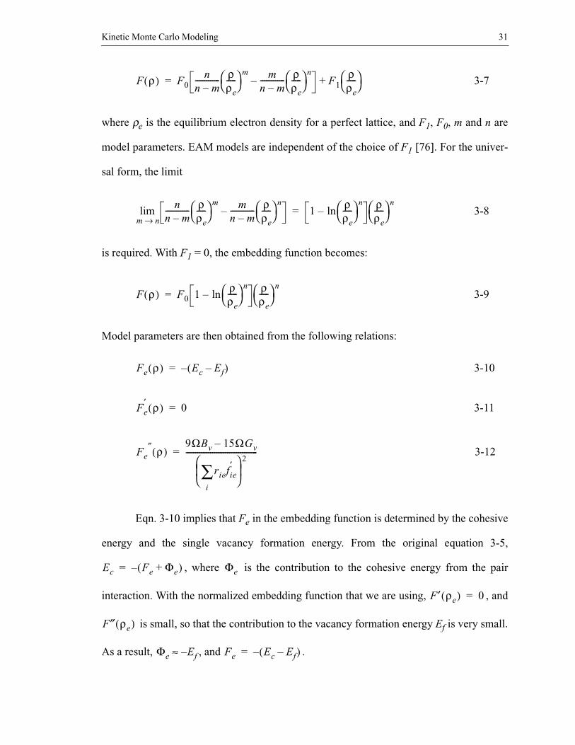
3-7
where ρe is the equilibrium electron density for a perfect lattice, and F1, F0, m and n are
model parameters. EAM models are independent of the choice of F1 [76]. For the univer-
sal form, the limit
3-8
is required. With F1 = 0, the embedding function becomes:
3-9
Model parameters are then obtained from the following relations:
3-10
3-11
3-12
Eqn. 3-10 implies that Fe in the embedding function is determined by the cohesive
energy and the single vacancy formation energy. From the original equation 3-5,
, where is the contribution to the cohesive energy from the pair
interaction. With the normalized embedding function that we are using, , and
is small, so that the contribution to the vacancy formation energy Ef is very small.
As a result, , and .
F ρ( ) F0n
n m–------------- ρ
ρe-----
m mn m–------------- ρ
ρe-----
n– F1
ρρe-----
+=
nn m–------------- ρ
ρe-----
m mn m–------------- ρ
ρe-----
n–
m n→lim 1
ρρe-----
nln–
ρρe-----
n=
F ρ( ) F0 1ρρe-----
nln–
ρρe-----
n=
Fe ρ( ) Ec Ef–( )–=
Fe′ ρ( ) 0=
Fe″ ρ( )
9ΩBv 15ΩGv–
riefie′
i
∑ 2
--------------------------------------=
Ec Fe Φe+( )–= Φe
F′ ρe( ) 0=
F″ ρe( )
Φe Ef–≈ Fe Ec Ef–( )–=

Kinetic Monte Carlo Modeling 32
Eqn. 3-11 results from the normalized embedding energies. Eqn. 3-12 is due to the
fitting conditions of relating the linear elastic constants to the EAM parameters by apply-
ing an infinitesimal homogeneous strain to a perfect pure crystal at equilibrium [76, 80].
Combining Eqns. 3-10 through 3-12 then gives the model parameters as follows:
3-13
3-14
3-15
where Ec is the cohesive energy, subscript ie denotes equilibrium value of the ith nearest
neighbor in a perfect lattice, and Ω is the atomic volume.
Next, we choose the electron density function f(r) and the two-body potential φ(r)
[81] as:
3-16
3-17
Where re is the equilibrium interatomic separation distance, rc is a cut-off distance.
As was explained earlier, with the normalized model we are using, the contribution
to the vacancy formation energy from the embedding function is small and we can assume
. Therefore for the nearest-neighboring model we have:
3-18
F0 Ec Ef–( )–=
F1 0=
n2
fie
i
∑
riefie′
i
∑------------------
2
9ΩBv 15ΩGv–
Ec Ef–--------------------------------------=
f r )( )re
r----
r rc–
re rc–---------------
2=
φ r( ) φe 2r rc–
re rc–---------------
33
r rc–
re rc–---------------
2––=
Φe Ef–≈
6φ re( ) Ef–=

Kinetic Monte Carlo Modeling 33
The normalization condition requires equilibrium at the perfect lattice setting:
3-19
The Voigt average shear moduli has to satisfy:
3-20
Also f(r) has to be continuous and smooth at the cutoff distance:
3-21
3-22
Equations 3-18 through 3-22 are the conditions we used to fit for the two-body potential.
The model parameters are finally determined by the following relations:
3-23
3-24
3-25
3-26
. 3-27
The EAM fitting parameters for two fcc metals (copper and nickel) are listed in
Table 3-1 [81].
6reφ′ re( ) 0=
6re2φ″ re( ) 15ΩGv=
φ rc( ) 0=
φ′ rc( ) 0=
φe16---Ef–=
re1
2-------a=
rc re 12Ef
5ΩGv--------------
1 2⁄+=
Fe Ec– Ef+=
nrc re–
rc re–---------------
9ΩBv 15ΩGv–
Ec Ef–--------------------------------------
1 2⁄
=

Kinetic Monte Carlo Modeling 34
Table 3-1 EAM physical and model parameters
The last two rows in the table show that when this model is applied to a close-packed two-
dimensional sheet, the equilibrium lattice constant is slightly reduced (2% for nickel, 4%
for copper) and the cohesive energy is reduced by about 20%. Figs. 3-1 to 3-3 show exam-
ples of the functional forms of f(r), F(ρ) and φ(r) for nickel.
Parameter Copper Nickel
Ω(Å3) 11.81 10.90
Ec(eV) 3.54 4.45
Ef(eV) 1.30 1.70
ΩBv(eV) 10.17 12.28
ΩGv(eV) 4.05 6.45
φe(eV) -0.216667 -0.283333
re(Å) 2.556162 2.489506
rc(Å) 3.472092 3.296827
Fe(eV) -2.24 -2.75
n 0.563224 0.312208
ρe 12 12
re(Å), 2D 2.44790 2.44567
Ec(eV), 2D 2.80547 3.55350

Kinetic Monte Carlo Modeling 35
3.5 Molecular Statics calculationsMolecular statics (MS) calculations can be used to estimate activation energies for
diffusion for various possible configurations [72]. In MS calculations the total energy of a
system of atoms is minimized as a function of all atoms’ coordinates. This is carried out
iteratively. In each iteration step the forces on all atoms are calculated, and the atoms are
moved in certain direction of the force over a distance proportional to the force. The pro-
ρ/ρe
Fig. 3.2. The embedding functionvs. electron density ratio for nickelmodel.
Fig. 3.1. The electron density func-tion f(r) vs. r for nickel model.
φr()
Fig. 3.3. The pair potential for nickel model.

Kinetic Monte Carlo Modeling 36
cess is repeated until the system energy difference between two consecutive moves is
smaller than a preset small number. The number of iterations needed for the system to con-
verge depends strongly on the choices of the direction and the proportionality constant in
the direction. If not chosen properly, convergence may be reached either only very slowly
(because the atoms hardly move) or the system may start to oscillate because the adjust-
ments overshoot. Thus speeding up convergence was the focus in the past. Use of the con-
jugate gradient method has simplified evaluation of the direction and proportionality
constants at each iteration step [82, 83].
The activation energy for an atom to jump to a neighboring site can then be calcu-
lated as follows. First the total energy of the system is minimized, allowing all atoms to
relax freely. Then the jumping atom is moved in small step along a line connecting its ini-
tial and final position. After each movement, the total energy of the system is calculated,
allowing the jumping atom to relax freely in the plane perpendicular to the jump direction,
and allowing all other atoms to relax freely. The diffusion path is then given by the succes-
sive positions of the jumping atom after relaxation. Note that the procedure described
above does not force the diffusion path to be a straight line. The height of the diffusion
barrier is given by the difference between the highest energy (after relaxation) between the
initial and final state, and the energy in the initial situation. Since thermal vibration of
atoms is not taken into account in MS calculations, the activation energies are calculated
for the case of T = 0 K.
Fig. 3.4 shows a sample energy barrier calculated by Johnson in this way for sur-
face migration in two-dimensional copper [81]. The configuration at the left is for a ledge
in a “surface” of tight-packed rows and at the right for a single atom one site away from
the ledge. From left to right the number of bonds changes from 3 to 2, and vice versa. This
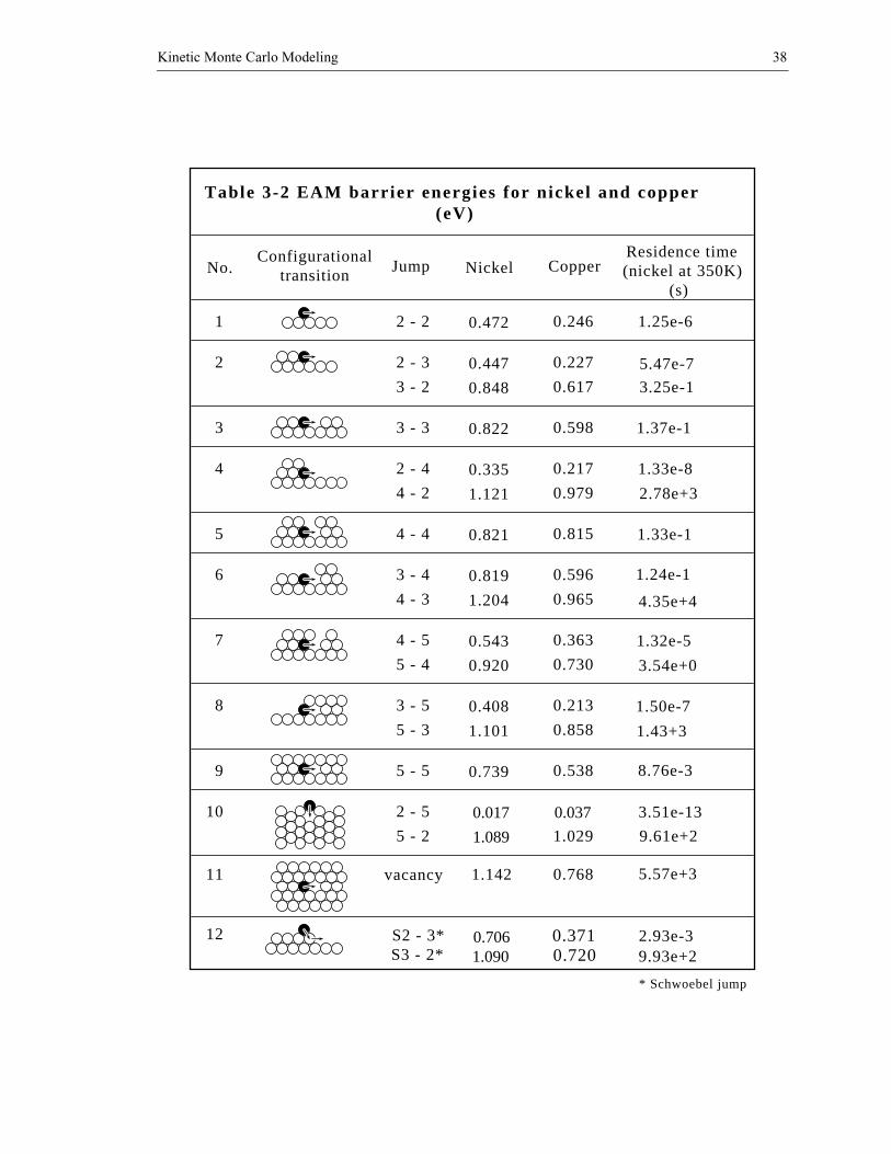
corresponds to run 2 in the table of activation energies, Table 3-2. It can be seen that diffu-
sion away from the ledge must overcome a barrier of 0.617 eV while diffusion toward the
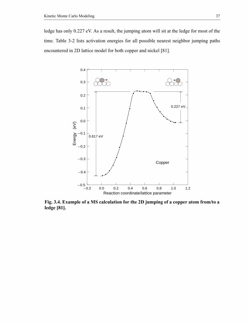
Kinetic Monte Carlo Modeling 37
ledge has only 0.227 eV. As a result, the jumping atom will sit at the ledge for most of the
time. Table 3-2 lists activation energies for all possible nearest neighbor jumping paths
encountered in 2D lattice model for both copper and nickel [81].
– 0.2 0.0 0.2 0.4 0.6 0.8 1.0 1.2Reaction coordinate/lattice parameter
Ene
rgy
(eV
)
– 0.5
– 0.4
– 0.3
– 0.2
– 0.1
0.0
0.1
0.2
0.3
0.4
0.617 eV
Copper
0.227 eV
Fig. 3.4. Example of a MS calculation for the 2D jumping of a copper atom from/to aledge [81].
Kinetic Monte Carlo Modeling 38
Table 3-2 EAM barrier energies for nickel and copper (eV)
Configurationaltransition
1 2 - 2
2 2 - 3
3 - 2
3 3 - 3
4 2 - 4
4 - 2
5
6 3 - 4
4 - 3
7 4 - 5
5 - 4
8 3 - 5
5 - 3
9 5 - 5
10 2 - 5
5 - 2
11
12
4 - 4
0.472
0.848
0.447
0.822
1.121
0.335
1.204
0.819
0.920
0.543
1.101
0.408
0.739
1.089
0.017
1.142
0.821
NickelJumpNo.
0.246
0.617
0.227
0.598
0.979
0.217
0.965
0.596
0.730
0.363
0.858
0.213
0.538
0.037
0.768
0.815
Copper
1.029
S2 - 3*
vacancy
* Schwoebel jump
S3 - 2*0.3710.720
0.7061.090
Residence time (nickel at 350K)
(s)
1.25e-6
9.93e+2
3.54e+0
1.32e-5
4.35e+4
1.24e-1
1.33e-1
2.78e+3
1.33e-8
1.37e-1
3.25e-1
5.47e-7
1.50e-7
1.43+3
8.76e-3
3.51e-13
9.61e+2
5.57e+3
2.93e-3

Kinetic Monte Carlo Modeling 39
3.6 Molecular dynamics calculations
Molecular dynamics, in its most straightforward realization, is an old idea. Given
the interaction potential and an initial configuration of N particles at time t, the resulting
forces acting on each atom are calculated. Newton equations of motion are then numeri-
cally solved for a small time interval ∆t under the assumption of constant force, obtaining
the system configuration at time t+∆t. In the limit ∆t → 0 the solution is exact. The proce-
dure can be iterated infinitely, and the evolution of the system can therefore be followed.
Suppose that a set of N classical particles have coordinates, ri, and masses mi, i =
1,..., N. The particles interact through a potential VN which, in most investigations is taken
to be:
, i, j = 1, 2,..., N, 3-28
where . Newton’s equations are then:
, i = 1,..., N, 3-29
and are solved numerically. As the system evolves in time it eventually reaches equilib-
rium conditions in its dynamical and structural properties. For practical reasons N is often
restricted to a few thousand and for small systems surface effects are obviously very
important. However, to simulate a bulk system the common practice is to use periodic
boundary conditions. These are obtained by periodically repeating a unit cell of volume W
containing the N particles by suitable translations. However the restriction that the MD
cell be kept constant in volume and in shape severely restricts the applicability of the
method to problems involving such factor as crystal structure transformations. In transfor-
mations changes in the shape of the cell most obviously play an essential role.
VN12--- φ rij( )
j j i≠,∑
i
∑=
rij ri rj–=
mri·· 1
rij----- dφ
drij--------rij
j i≠∑=

Kinetic Monte Carlo Modeling 40
In order to overcome this difficulty, Andersen [84] has shown how MD calcula-
tions can be modified to study systems under constant pressure by introducing the volume
of the system as an additional dynamical variable. Parrinello and Rahman [85] have mod-
ified the method so as to allow for changes in volume and shape of the MD cell containing
a system of particles under constant external hydrostatic pressure, whereas Andersen’s
method only allowed changes in the volume of the MD cell but not in its shape.
The implementation of MD is often based on the equations of motion derived by
the classical Lagrangian. Thus the three cases described above in Lagrangian forms can be
listed below.
1) The traditional Lagrangian:
3-30
Periodic boundary conditions are applied, most often, in the form of a repeating cubic cell
of volume L3. The point to note is that L is a constant and can be used as the unit of length.
2) The introduction of a time-dependent volume W(t) by Andersen who used
, 3-31
where . Periodic boundary conditions of the usual kind give a pulsating cubic
box which changes in time according to a Lagrangian equation of motion [84]. The con-
stant C, a coupling parameter, can be thought as the mass of a piston [84]. The mass deter-
mines the relaxation time for recovery from an imbalance between the external pressure
and the internal stress. An appropriate choice for the value of W can make this relaxation
time of the same order of magnitude as that of the relaxation of a small portion of a much
L112--- mivi
2VN–
i
N
∑=
L2 Ω2 3⁄ 12--- ms·i
2VN–
12---CΩ
· 2pΩ–+
i
N
∑=
si ri Ω1 3⁄⁄=

Kinetic Monte Carlo Modeling 41
larger sample. However, if one is interested only in static averages, W can be chosen on
the basis of computational convenience. In fact, in classical statistical mechanics, the equi-
librium properties of a system are independent of the masses of its constituent parts.
3) The introduction of a time-dependent shape by Parrinello and Rahman [85] who
used vectors a(t), b(t), and c(t) to define the molecular dynamics cell and used (a prime
indicating the transpose)
, 3-32
where ri = hsi, h(t) = a,b,c, G = h’h, and W is a mass associated with the coor-
dinates . Periodic boundary conditions of the usual kind give a pulsating molecular
dynamics cell of arbitrary shape which changes according to Lagrangian equations of
motion. This is when only hydrostatic pressure p is applied. The introduction of an aniso-
tropic stress tensor S in place of p has been given by Parrinello and Rahman as well [85].
Since the earliest days’ work by Vineyard and coworkers [86] on dynamics of radi-
ation damage and Verlet [87] on computer “experiments” on classical fluids, the MD sim-
ulation has seen widespread use in materials science community. It has been used to
simulate melting of silicon, crystal growth, crack propagation, ion bombardment, multi-
layer deposition, to name just a few areas.
However, a full MD atomistic simulation of vapor-phase crystal growth is actually
extremely difficult. Two factors that enter into this are the large number of vapor atoms
that must be added to the substrate to grow a new layer, and the length of time that must
pass between introduction of new vapor atoms. This latter factor is the primary difficulty,
as the enormous disparity in time scales between experimental and simulated time scales
(perhaps 8-10 orders of magnitude) makes such simulations potentially misleading.
L312--- mis
·i′Gs· i VN–
12---WTrh· ′h· pΩ–+
i
N
∑=
Ω h=
hλµ

Kinetic Monte Carlo Modeling 42
In this work, the purpose employing MD technique is to use its strength of physical
dynamics to extract energetic interaction data for kMC simulation. We modified the
DYNAMO MD program [88] in which the Lagrangian derived equations of motion were
integrated to simulate the energetic atom’s interaction with the substrate. More details on
the energy data extraction are given in chapter seven.