50

CHAPTER 3

DESIGN OF MOTORCYCLE DISC BRAKE

3.1 BASIC BRAKE SYSTEM DESIGN CONSIDERATIONS

In most cases the brake engineer has the following data available when designing the brakes of a vehicle:

Empty and loaded vehicle weight

Static weight distribution lightly and fully laden

Wheel base

Center of gravity height lightly and fully laden

Tyre and rim size

3.2 MEASUREMENT OF CENTRE OF GRAVITY (CG)

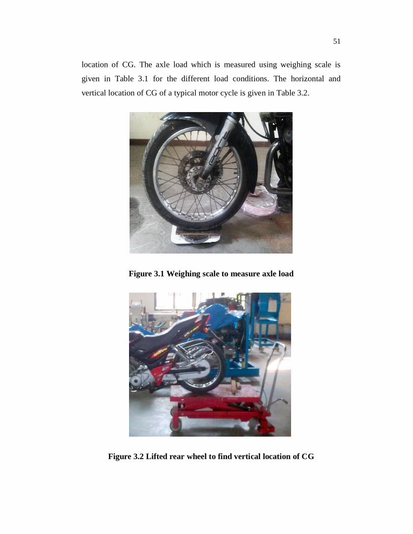
The motorcycle’s front wheel load distribution is calculated by placing the front wheel on a weighing scale. After finding the front wheel load distribution, an application of balance moment about the rear axle is taken to find the horizontal location of centre of gravity (CG) of the motor cycle. Figure 3.1 shows the reading which is taken using weighing scale.

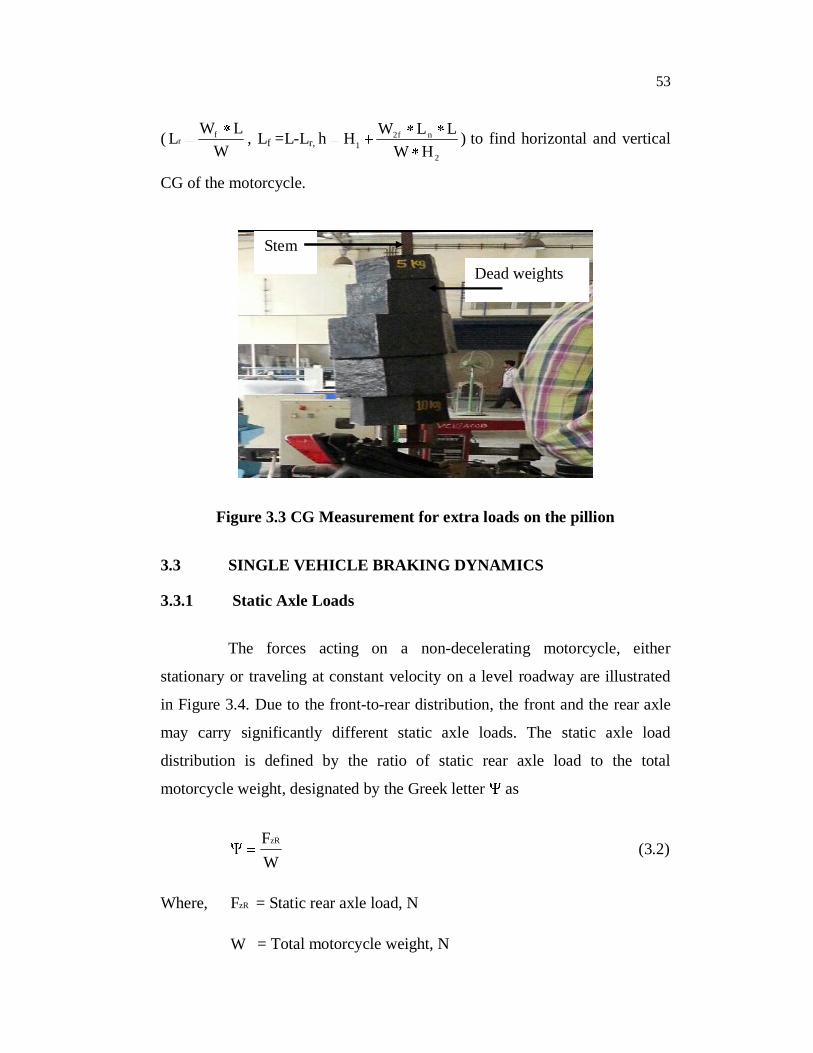
The vertical location of CG is measured by lifting the rear wheel to

a certain height and the front axle weight is noted down by using weighing

scale. After taking required readings, a formula (Derived in Appendix 1)

which is given in Equation 3.1 is used to find the vertical location of CG of

the motorcycle. Figure 3.2 shows the lifted rear axle for finding the vertical

51

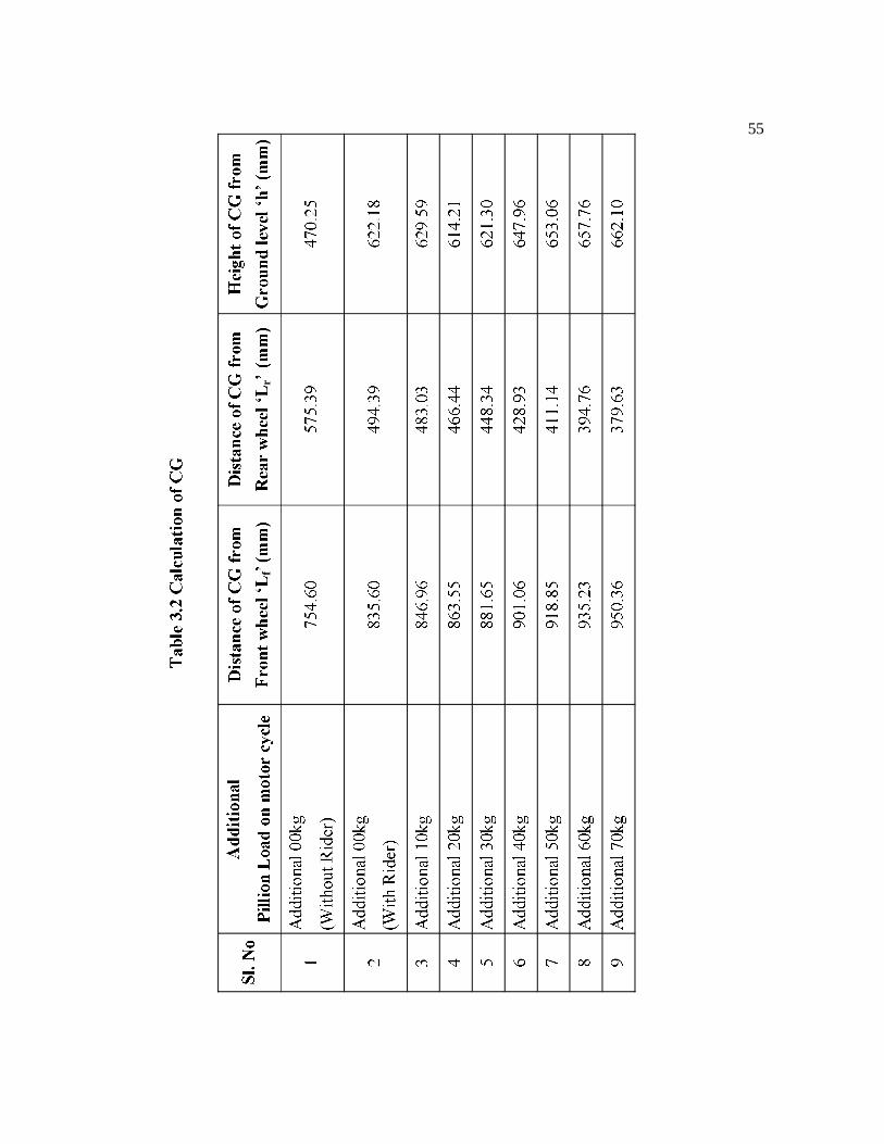
location of CG. The axle load which is measured using weighing scale is

given in Table 3.1 for the different load conditions. The horizontal and

vertical location of CG of a typical motor cycle is given in Table 3.2.

Figure 3.1 Weighing scale to measure axle load

Figure 3.2 Lifted rear wheel to find vertical location of CG

52

Height of CG (h) = 2H*W

nL*L*2fW1H (3.1)

Where

Wf = Weight on front axle when the motorcycle is level

Wr = Weight on rear axle when the motorcycle is level

Wlf = Weight on front axle when the motorcycle’s rear wheel is lifted

W = Total motorcycle weight = Wf +Wr

W2f = Weight added on front axle because of rear wheel lift = Wlf - Wf

L = Length of wheelbase while the motorcycle is level = 1330 mm

H1= Height of front hub off the ground = 300 mm

H2= Height of rear wheel hub above the front wheel hub

(How high the rear-end has been lifted = 355mm)

Ln= New wheelbase when the motor cycle rear wheel is lifted

Ln= 2

22 HL

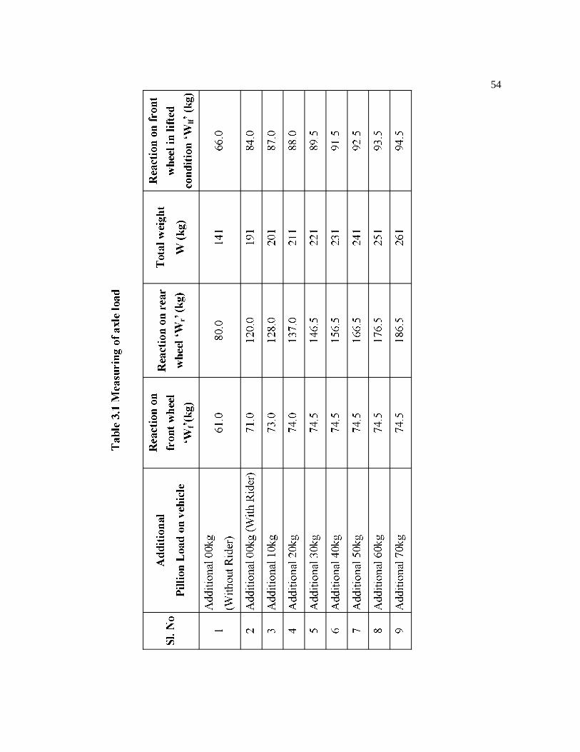
An iron stem as shown in Figure 3.3 is attached directly above the

position of the axle (The line of action of load is passing perpendicular to the

axis of axle and through the rear tyre contact patch with the ground). The

stem is rigidly fixed with motorcycle frame after removing the seat. Then a

dead weight which has a hole in its centre is inserted into the stem. The

weight of the each dead weight is 10kg. All dead weights are added in the

same manner for taking readings which are substituted in the formulas

53

(W

LWL fr , Lf =L-Lr,

2

nf21 HW

LLWHh ) to find horizontal and vertical

CG of the motorcycle.

Figure 3.3 CG Measurement for extra loads on the pillion

3.3 SINGLE VEHICLE BRAKING DYNAMICS

3.3.1 Static Axle Loads

The forces acting on a non-decelerating motorcycle, either

stationary or traveling at constant velocity on a level roadway are illustrated

in Figure 3.4. Due to the front-to-rear distribution, the front and the rear axle

may carry significantly different static axle loads. The static axle load

distribution is defined by the ratio of static rear axle load to the total

motorcycle weight, designated by the Greek letter as

WFzR

(3.2)

Where, zRF = Static rear axle load, N

W = Total motorcycle weight, N

Stem

Dead weights

54

fr

lf

55

fr

56

The relative static front axle load is given by

WF1 zF (3.3)

Where

zFF = Static front axle load ,N

The typical motorcycle has values for the empty conditions as

high as 0.63, indicating that only 63% of the total weight is carried by the rear

axle and that for loaded condition is 0.72.

Application of moment balance about the front axle of the

stationary motorcycle shown in Figure 3.4 yields

Figure 3.4 Static axle forces

LFWL zRf (3.4)

57

Where

L = Length of wheel base while the motorcycle is level, m

fL = Horizontal distance from centre of gravity to front axle, m

W = Total motorcycle weight = mg, N

Solved for the horizontal distance fL between front axle and CG

LLWFL zR

f , m (3.5)

Similarly, for the horizontal distance rL between the rear axle and the CG

rL = (1- ) L , m (3.6)

3.3.2 Dynamic Axle Loads

When the brakes are applied, the torque developed by the wheel

brake is resisted by the tyre circumference where it comes in contact with the

ground. Prior to brake lockup, the magnitude of the braking forces is a direct

function of the torque produced by the wheel brake. For hydraulic brakes,

Equation (3.7) is used for determining the actual braking forces.

RrBFA)P(PF c0Lx , N (3.7)

Where

xF = Braking force, N

LP = Hydraulic brake line pressure, N/m2

58

0P = Pushout pressure , required to bring brake pads in

contact with disc, N/m2

A = Caliper cylinder area, m2

c = Caliper cylinder efficiency

BF = Brake factor

r = Effective radius of disc, m

R = Effective rolling radius of tyre, m

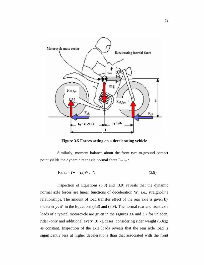
The forces acting on a motorcycle decelerating on a level road are

illustrated in Figure 3.5. Application of moment balance about the rear tyre-

to-ground contact patch yields the dynamic normal force dynzF,F on the front

axle:

a)W(1F dynzF, , N (3.8)

Where

a =W

F totalx, = Motorcycle deceleration, g-units

ltotax,F = total braking force, N

zRF = Static rear axle load, N

W = Total motorcycle weight, N

= CG height (h) divided by wheel base (L)

WFzR

59

Figure 3.5 Forces acting on a decelerating vehicle

Similarly, moment balance about the front tyre-to-ground contact

point yields the dynamic rear axle normal force dynzR,F :

a)WF dynzR, , N (3.9)

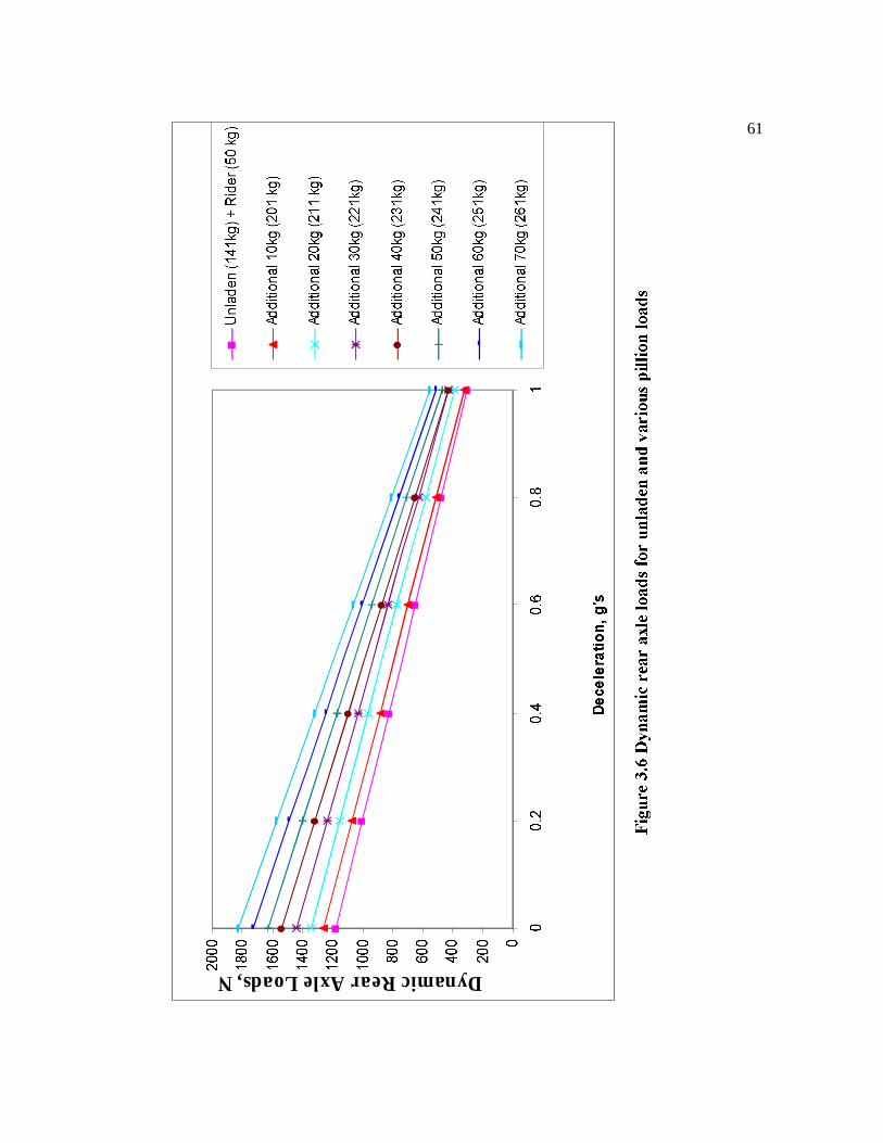
Inspection of Equations (3.8) and (3.9) reveals that the dynamic

normal axle forces are linear functions of deceleration ‘a’, i.e., straight-line

relationships. The amount of load transfer effect of the rear axle is given by

the term aW in the Equations (3.8) and (3.9). The normal rear and front axle

loads of a typical motorcycle are given in the Figures 3.6 and 3.7 for unladen,

rider -only and additional every 10 kg cases, considering rider weight (50kg)

as constant. Inspection of the axle loads reveals that the rear axle load is

significantly less at higher decelerations than that associated with the front

L

60

axle. For example, the rear axle load has decreased from a static load of 785 N

to only 295 N for a 1g stop at unladen (141 kg) condition, while the front load

has increased from 589 N to 1080 N.

3.4 OPTIMUM BRAKING FORCES

3.4.1 Braking Traction Coefficient

The wheel brake torques generate braking or traction forces

between the tyre and the ground. The ratio of braking force to dynamic axle

load is defined as the traction coefficient Ti

dynzi,

xi

FF

Ti (3.10)

Where

xiF = Dynamic axle braking force, N

dyn,ziF = dynamic axle normal force, N

i = designates front (F) or rear axle (R)

The traction coefficient is the level of tyre-road friction needed by

the braked tyre so that it will just not lock up. The traction coefficient varies

as either braking force or dynamic axle normal force change and,

consequently, is a vehicle and deceleration-dependent parameter. In general,

the front and rear axle traction coefficient will be different. Only when the

numerical values of traction and tyre road friction coefficients are equal does

the tire lock up.

61

DynamicRearAxleLoads,N

62

DynamicFrontAxleloads,N

63

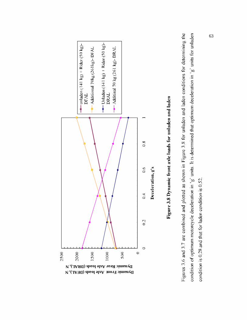
DynamicFrontAxleloads(DFAL),NDynamicRearAxleloads(DRAL),N

64

3.4.2 Dynamic Braking Forces

Multiplication of the dynamic axle loads by the traction coefficient

yields the dynamic braking forces xFF for the front axle:

TFxF a)W(1F , N (3.11)

Similarly the dynamic braking force xRF for the rear axle is given

by

RTxR a)WF , N (3.12)

Where,

TF = Front traction coefficient.

RT = Rear traction coefficient.

The tyre-road friction coefficient F or R , existing at either the

front or the rear tyre, is indicative of the ability of a road surface to allow

traction to be produced for a given tyre and, as such, is a fixed number. A

braked tyre will continue to rotate as long as the traction coefficient is less

than the tyre-road friction coefficient, otherwise it will lock up. At the

moment of incipient tyre lock up, the traction coefficient equals the tyre - road

friction coefficient. When both the axles of the motorcycle are braked at

sufficient levels so that the front and the rear wheels are operating at incipient

or peak friction conditions, then the maximum traction capacity between the

tyre road system is utilized. Under these conditions the motorcycle

deceleration will be a maximum, since the traction coefficients of front and

rear are equal, and are also equal to the motorcycle deceleration measured in

g-units.

65

3.4.3 Optimum Straight-Line Braking

For straight-line braking on a level surface in the absence of any

aerodynamic effects and rolling resistance of tyre, optimum braking in terms

of maximizing motorcycle deceleration is defined by

aRF (3.13)

Where,

a = Motorcycle deceleration, g-units.

F = Front tyre-road friction coefficient.

R = Rear tyre-road friction coefficient.

The optimum braking forces may be determined by setting the

traction coefficient equal to motorcycle deceleration in Equations (3.11) and

(3.12), resulting in the optimum braking force optxF,F on the front axle

aa)W(1F optxF, , N (3.14)

And the optimum braking force FxR,opt on the rear axle

a)WaF optxR, , N (3.15)

Inspection of Equations (3.14) and (3.15) reveals a quadratic

relationship relative to deceleration ‘a’. The graphical representation is a

parabola as illustrated in Figure 3.9 for different pillion loads on the motor

cycle. Any point on the curve represents an optimum point identified by

deceleration equal to friction coefficient. Inspection of the empty case reveals

that for decelerations greater than 0.8 to 1g , optimum rear braking begins to

decrease due to the significant load transfer onto the front axle. For the loaded

case, the higher static rear axle load yields an increasing optimum rear brake

force with higher deceleration.

66

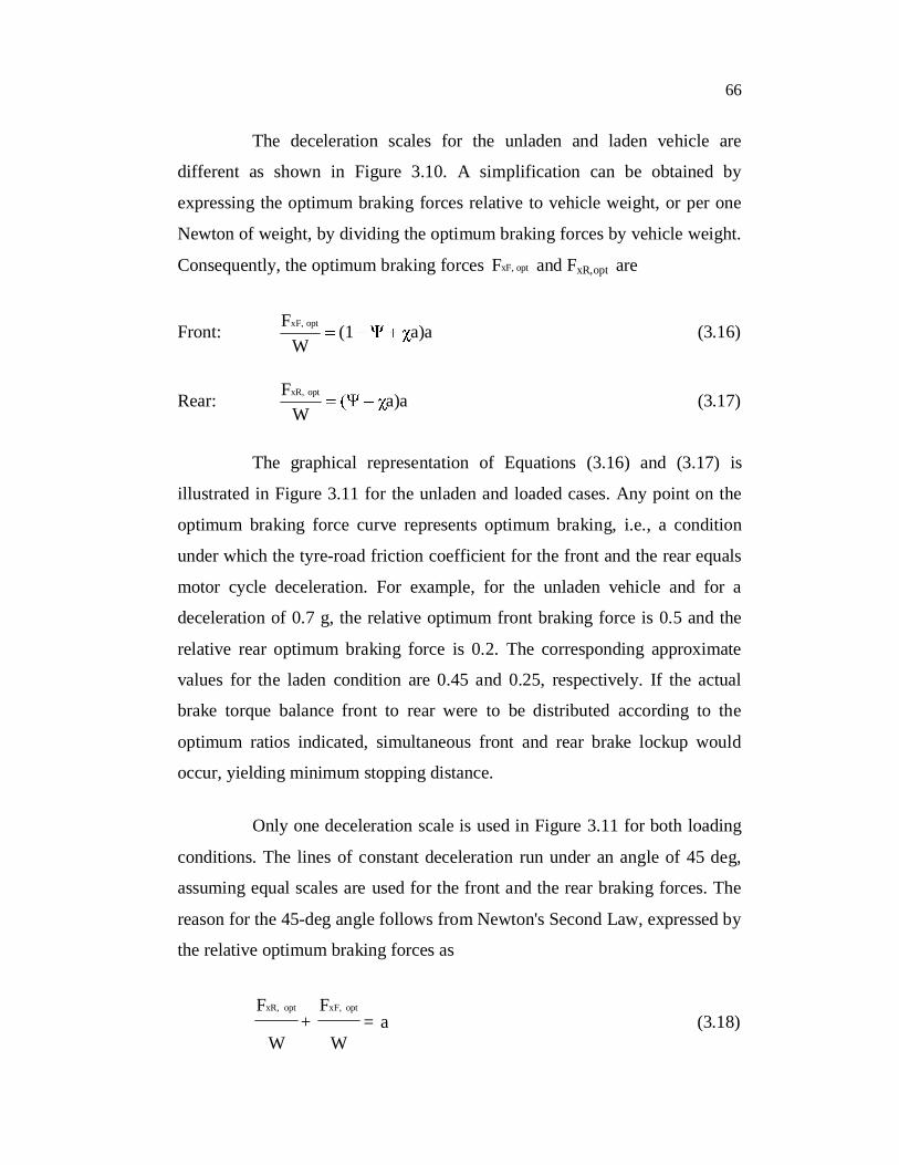
The deceleration scales for the unladen and laden vehicle are

different as shown in Figure 3.10. A simplification can be obtained by

expressing the optimum braking forces relative to vehicle weight, or per one

Newton of weight, by dividing the optimum braking forces by vehicle weight.

Consequently, the optimum braking forces optxF,F and FxR,opt are

Front: a)a(1W

F optxF, (3.16)

Rear: a)aW

F optxR, (3.17)

The graphical representation of Equations (3.16) and (3.17) is

illustrated in Figure 3.11 for the unladen and loaded cases. Any point on the

optimum braking force curve represents optimum braking, i.e., a condition

under which the tyre-road friction coefficient for the front and the rear equals

motor cycle deceleration. For example, for the unladen vehicle and for a

deceleration of 0.7 g, the relative optimum front braking force is 0.5 and the

relative rear optimum braking force is 0.2. The corresponding approximate

values for the laden condition are 0.45 and 0.25, respectively. If the actual

brake torque balance front to rear were to be distributed according to the

optimum ratios indicated, simultaneous front and rear brake lockup would

occur, yielding minimum stopping distance.

Only one deceleration scale is used in Figure 3.11 for both loading

conditions. The lines of constant deceleration run under an angle of 45 deg,

assuming equal scales are used for the front and the rear braking forces. The

reason for the 45-deg angle follows from Newton's Second Law, expressed by

the relative optimum braking forces as

W

F optxR,

+W

F optxF,

= a (3.18)

67

DynamicFrontAxleBrakeForceFxF,dynN

68

DynamicFrontAxleBrakeForce,FxF,dynN

69

Inspection of Figure 3.11 reveals, for example, for the 0.8

g-deceleration line substituted into Equation (3.18), that for the unladen case:

0.58 + 0.22 = 0.8; and for the laden case: 0.55 + 0.25 = 0.8. The numerical

values indicate that the front braking force decreased by 0.58 - 0.55 = 0.03 on

the vertical axis, which is the increase experienced by the rear braking force

on the horizontal axis. The result is a right-angled triangle with two sides of

equal distance, namely the vertical and horizontal components, thus yielding a

45-degree slope for the deceleration lines.

Inspection of Equations (3.16) and (3.17) reveals that the optimum

braking forces are only a function of the particular motor cycle geometry and

weight data, i.e., and , and vehicle deceleration ‘a’. They are not a function

of the brake system hardware that has been installed.

To better match actual with optimum braking forces, it becomes

convenient to eliminate motor cycle deceleration by solving Equation (3.16)

for deceleration ‘ a ’, and substituting into Equation (3.18). The result is the

general optimum braking forces equation.

Figure 3.11 Normalized dynamic brake forces

Brake balance ( ) = 0.3, Fixed

70

WF1

WF1

22)(1

WF optxF,optxF,optxR, (3.19)

Equation (3.19) allows computation of the appropriate optimum

rear axle braking force associated with an arbitrarily specified (optimum)

front braking force.

The graphical representation of Equation (3.19) is that of a parabola

illustrated in Figure 3.12. The optimum curve located in the upper right

quadrant represents braking, the lower left acceleration. Only the braking

quadrant and then only the section exhibiting deceleration ranges of interest

are of direct importance to brake engineers. The optimum curves shown in

Figure 3.12 represent the section of interest relative to deceleration ranges

encountered frequently.

The entire optimum braking/acceleration forces diagram, however,

is used to develop useful insight and design methods for matching optimum

and actual braking forces for brake design purposes. In addition, the methods

will also be used in the reconstruction of actual motorcycle accidents

involving braking and loss of directional stability due to premature rear brake

lock up.

3.5 LINES OF CONSTANT FRICTION COEFFICIENT

For increasing deceleration, assuming that the tyre-road friction is

high enough, the optimum braking of the rear axle begins to decrease and

reaches zero where it intercepts the front braking axis. At this point the

deceleration of the motorcycle is sufficiently high that the rear axle begins to

lift off the ground due to excessive load transfer effect.

71

72

Similarly, in the case of increasing acceleration, the front axle

begins to lift off the ground when the optimum acceleration curve intercepts

the rear braking force axis.

The zero point on the front braking force axis is determined by

setting the relative rear axle braking force equal to zero in Equation (3.19) and

solving for the relative front braking force, resulting in

)(1WF

0W

F xRoptxF,

Similarly, setting the relative front axle braking force equal to zero

in Equation (3.19) yields

WF

0W

F xFoptxR,

Any point on the optimum braking forces curve represents the

condition under which the front and the rear tyre-road friction coefficients are

equal to each other as well as to the deceleration of the motor cycle. Under

these conditions all available tyre-road friction is utilized for vehicle

deceleration. For example, at the 0.7 g point the front and the rear tyre-road

friction coefficients are also equal to 0.7.

At the respective zero points, the tyre traction forces, either braking

or accelerating, are zero regardless of the level of friction coefficient existing

between the tyre and the ground due to the normal forces between the tyre and

the ground being zero.

A straight line connecting the zero point )1( and a point of

the optimum force curve represents a condition of constant coefficient of

73

friction between the front tyre and the ground. For example, connecting the

zero point with the 0.7 g optimum point establishes a line of front tyre friction

coefficient of 0.7 constant along the entire line.

Similarly, by connecting the rear zero point with points on the

optimum curve, lines of constant rear tyre friction coefficient are obtained.

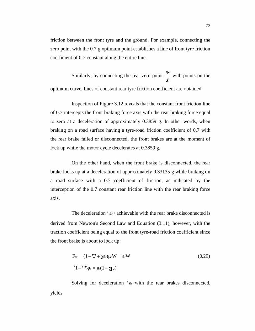
Inspection of Figure 3.12 reveals that the constant front friction line

of 0.7 intercepts the front braking force axis with the rear braking force equal

to zero at a deceleration of approximately 0.3859 g. In other words, when

braking on a road surface having a tyre-road friction coefficient of 0.7 with

the rear brake failed or disconnected, the front brakes are at the moment of

lock up while the motor cycle decelerates at 0.3859 g.

On the other hand, when the front brake is disconnected, the rear

brake locks up at a deceleration of approximately 0.33135 g while braking on

a road surface with a 0.7 coefficient of friction, as indicated by the

interception of the 0.7 constant rear friction line with the rear braking force

axis.

The deceleration ‘ Fa ’ achievable with the rear brake disconnected is

derived from Newton's Second Law and Equation (3.11), however, with the

traction coefficient being equal to the front tyre-road friction coefficient since

the front brake is about to lock up:

WaWa(1F FFFxF (3.20)

)(1a(1 FFF

Solving for deceleration ‘ Fa ’with the rear brakes disconnected,

yields

74

F

F

1(1a F , g-units (3.21)

A similar derivation yields the deceleration ‘ Ra ’ with the front

brakes disconnected:

R

R

1a R (3.22)

where F = Front tyre-road friction coefficient

Fa = Deceleration with the rear brake disconnected in ‘g’uints

R = Rear tyre-road friction coefficient

Ra = Deceleration with the front brake disconnected in ‘g’ units

It becomes convenient to use Equations (3.21) and (3.22) along

with the optimum points to draw the lines of constant friction coefficient

rather than using the zero points.

Figure 3.13 shows the lines of constant friction coefficient for the

motor cycle under loaded condition.

It is concluded that normalized dynamic rear axle load is increased

from 0.33135 to 0.37069 based on the motorcycle geometry. Hence the

effective disc radius may be varied for controlling rear braking force based on

pillion load in the motorcycle. The required rear wheel braking force for

various pillion load is found out using Figures which are shown in

Appendices (A3.1) to (A8.1).

75

76

3.6 CALCULATION OF EFFECTIVE DISC RADIUS

RrBFA)P(PF c0LxR , N (3.23)

Where xRF = Dynamic braking force for rear axle (calculated from Figure 3.12 and Figure 3.13 for unladen and laden condition respectively).

LP = Hydraulic brake line pressure (Approximately 6.20 N/mm2).

0P = Pushout pressure , required to bring brake pads in contact

with the disc (0.05 N/mm2).

A = Caliper cylinder area ( Diameter 32mm).

c = Caliper cylinder efficiency ( Assumed 0.98).

BF = Brake factor ( Assumed 0.7).

r = Effective radius of disc.

R = Effective rolling radius of tire (300 mm).

When the brake is applied, the braking force is linearly varied with

time. But, in this research work the maximum braking force between tyre and

ground (the product of normal reaction on wheel and friction coefficient

between tyre and ground) is controlled based on pillion load on the two-

wheeler by changing the effective radius of disc. For brakes without a booster,

the brake system should be designed so that for a maximum pedal force of

425 to 489 N, a theoretical deceleration of 1g is achieved when the vehicle is

loaded at GVW (Gross vehicle weight).

mc

ppp

L A*l*FP (3.24)

77

Where,

LP = Hydraulic brake line pressure ( Measured 6.2 N/mm2).

pF = Pedal force, N

pl = Pedal lever ratio =145/35= 4.142.

p = Pedal lever efficiency = 0.8 (approximately).

mcA = Master cylinder bore area = 3.14*17*17/4 = 226.98 mm2.

Pedal lever efficiency is defined as the ratio of the force developed in the pushrod of the master cylinder to the force applied in the brake pedal. In general there would be some losses due to the friction between master cylinder piston and cylinder. Moreover the return spring connected to the brake pedal develops a restoring force (opposite to applied pedal force) that must be balanced. Hence the net force acting on the master cylinder pushrod is less than the applied force.

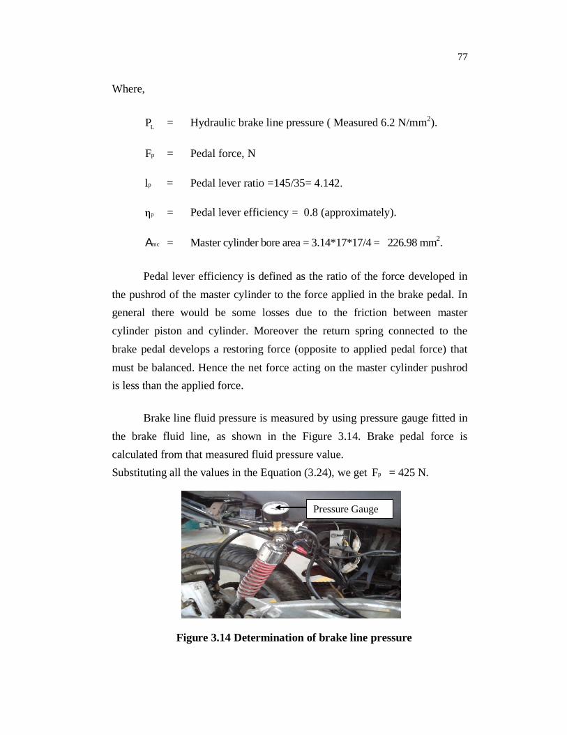
Brake line fluid pressure is measured by using pressure gauge fitted in the brake fluid line, as shown in the Figure 3.14. Brake pedal force is calculated from that measured fluid pressure value. Substituting all the values in the Equation (3.24), we get pF = 425 N.

Figure 3.14 Determination of brake line pressure

Pressure Gauge

78

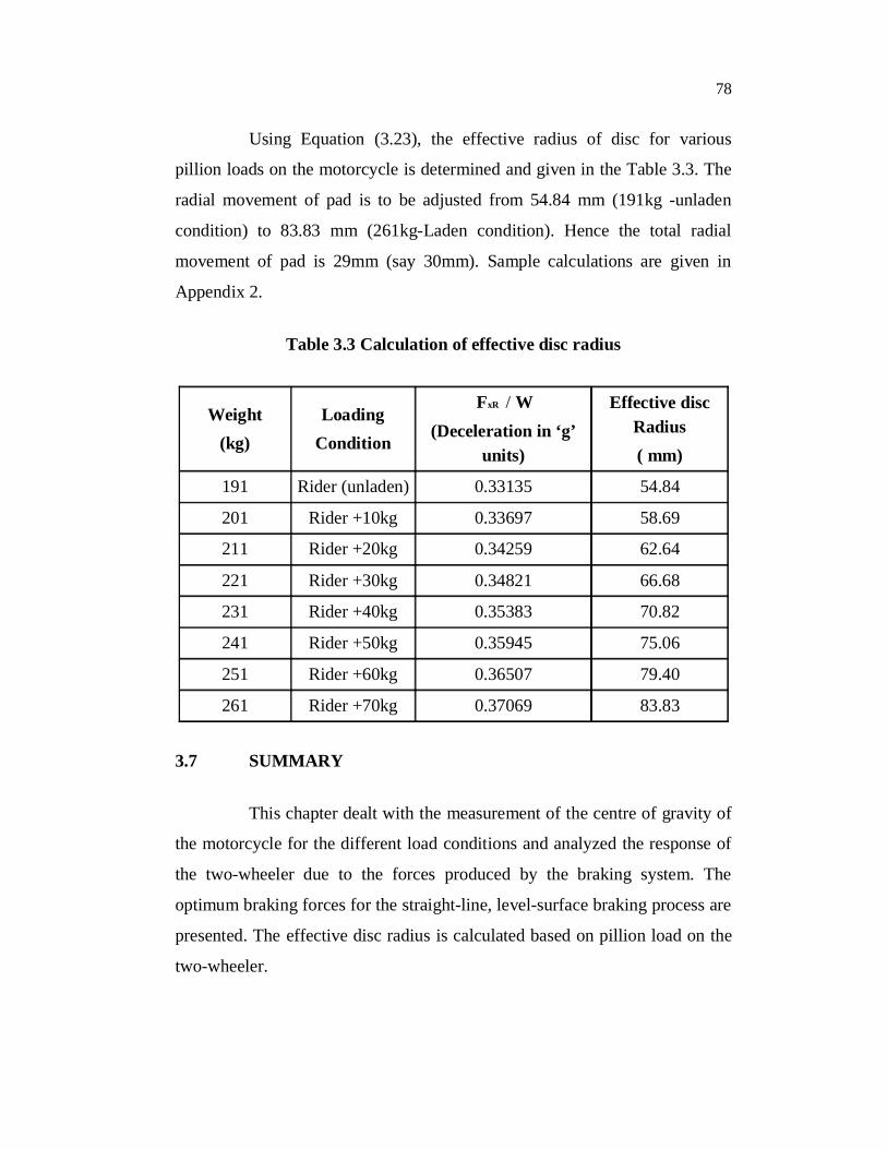
Using Equation (3.23), the effective radius of disc for various

pillion loads on the motorcycle is determined and given in the Table 3.3. The

radial movement of pad is to be adjusted from 54.84 mm (191kg -unladen

condition) to 83.83 mm (261kg-Laden condition). Hence the total radial

movement of pad is 29mm (say 30mm). Sample calculations are given in

Appendix 2.

Table 3.3 Calculation of effective disc radius

Weight (kg)

Loading Condition

xRF / W (Deceleration in ‘g’

units)

Effective disc Radius ( mm)

191 Rider (unladen) 0.33135 54.84

201 Rider +10kg 0.33697 58.69

211 Rider +20kg 0.34259 62.64

221 Rider +30kg 0.34821 66.68

231 Rider +40kg 0.35383 70.82

241 Rider +50kg 0.35945 75.06

251 Rider +60kg 0.36507 79.40

261 Rider +70kg 0.37069 83.83

3.7 SUMMARY

This chapter dealt with the measurement of the centre of gravity of

the motorcycle for the different load conditions and analyzed the response of

the two-wheeler due to the forces produced by the braking system. The

optimum braking forces for the straight-line, level-surface braking process are

presented. The effective disc radius is calculated based on pillion load on the

two-wheeler.