Corporate Dimensions of Risk

79

Introduction to Finance

by George W. Blazenko

All Rights Reserved © 2008, 2014

Chapter 3 Corporate

Dimensions of Risk “The biggest risk is not taking any risk... In a world quickly changing, the only strategy

guaranteed to fail is not taking risks.” Mark Zuckerberg.

“Most of us would rather risk catastrophe than read the directions.” Mignon McLaughlin,

US journalist and author

“Risk comes from not knowing what you're doing.” Warren Buffett

Introduction to Finance

80

Chapter Three Contents

(3.1) Introduction ............................................................................. 81

(3.2) EBITDA and Operating Leverage ................................... 81

3.2.1 THE DEGREE OF OPERATING LEVERAGE 85

3.2.2 OPERATING EFFICIENCY AND OPERATING RISK 86

3.2.3 EBITDA MARGIN AS AN INVERSE RISK MEASURE 89

3.2.4 BREAK EVEN SALES AND OPERATING RISK 90

(3.3) Estimating Contribution Per Dollar Sales ..................... 91

3.3.1 EBITDA RISK AND REVENUES 93

3.3.2 CANADIAN PACIFIC RAILWAY 94

(3.4) Customer Price Sensitivity and Break-Even $SALES ............ 96

(3.5) Financial Leverage .................................................................... 99

3.5.1 ROE VARIABILITY AND DEBT FINANCING 102

(3.6) Summary .................................................................................. 105

(3.7) Suggested Readings .................................................................. 106

(3.8) Problems ................................................................................... 107

(3.9) Chapter Index ........................................................................... 114

Corporate Dimensions of Risk

81

(3.1) INTRODUCTION Title Page

In chapter one, we identified four questions a financial analyst investigates for any investment:

expenditure, return, risk, and “is this a good investment.” In chapter two, we studied how to

measure business returns. In this chapter, we study two corporate risk measures: operating and

financial leverage. In later chapters, we study opportunity cost rates of return that when we

combine all of our studies will allow us to answer the “is this a good investment” question for

businesses.

(3.1) EBITDA and Operating Leverage Title Page

In chapter two, we defined EBITDA as Sales less Cost of Sales less General, and Administrative

Expenses (before depreciation and amortization The financial statement decomposition of

expenses into Cost of Sales and General and Administrative Expenses is a convenient way to

measure operating efficiency. In addition, there are other useful ways to decompose expenses.

A second decomposition is to separate fixed expenses from variable expenses. Variable

expenses vary with the level of a firm’s sales and fixed expenses do not. The usual financial

statement decomposition of expenses into Cost of Sales versus General and Administrative

Expenses is not the same as the decomposition of expenses into variable expenses versus fixed

expenses because some commercial (general) expenses vary with the level of sales. One

example is advertising: higher sales should be associated with higher advertising expenditure.

Using the variable and fixed decomposition of expenses, we can represent EBITDA as1:

EBITDA = SALES VC FC

1 For a multi-product firm, contribution margin times sales must be summed over all of the products and services

sold by the firm.

Introduction to Finance

82

where VC is total variable cost and FC is fixed cost per period. The measurement interval for

EBITDA and SALES can be daily, weekly, monthly, yearly or any other period. In practice, for

convenience, we generally measure EBITDA over the fiscal reporting period of a firm like, for

example, a quarter or a year.

Total contribution is SALES less total variable cost, VC. If we divide total contribution by

SALES, we get contribution margin per dollar of sales,

( )CM$

SALES VC

SALES

Contribution margin per dollar sales, / $CM , is the increment to EBITDA that arises from an

additional dollar of sales (before fixed costs). We presume / $CM is a constant in the short-

term. In particular, / $CM does not vary with a firm’s sales activity. Initially this presumption

might be hard to accept because both the numerator and the denominator in the above formula

depend upon SALES. However, we justify this presumption in a numerical example shortly.

We can write EBITDA with / $CM ,

CMEBITDA= - FC$

SALES

A similar expression for EBITDA but with CM/unit and unit sales is

UnitSalesCMEBITDA = - FCunit

CM/unit is the contribution to EBITDA of an extra unit sale.

Corporate Dimensions of Risk

83

In Chapter 2, we defined EBITDA margin as EBITDA2 divided by dollar sales. Using the

fixed/variable decomposition of expenses, we can represent the EBITDA margin as:

CM SALES - FC$

Margin = SALES

EBITDA

EBITDA margin is the increment to EBITDA of an extra $SALES after fixed costs.

Consider the following example:

Assumed Facts for ABC Company

Unit price $2.50

Unit variable cost $2.00

Fixed Costs $40,000 per month

Units sold 250,000 units per month

For ABC Company,

SALES=$2.5*250,000=$625,000/month

VC=$2.0*250,000=$500,000/month

unit

CM = $2.50 – $2.00 = $0.50

(625,000 500,000)CM$ 625,000

(2.5 2.0)0.2

2.5

2As a general rule, in applying this representation for actual firms, you should use EBITDA before other income like,

for example, investment income.

Introduction to Finance

84

The incremental impact of one unit sale on the firm’s EBITDA is $0.50. The incremental impact

of one dollar of sales on EBITDA is $0.20.

The above calculation illustrates why we can presume CM$

is a constant in the short-term. We

can calculate CM$

as total contribution (SALES-VC) divided by SALES. We can also calculate

CM$

as unit contribution (unit product price less unit variable cost) divided by unit product

price (that is, 2.5 2.0

2.5

). Unit product price is the price we require of our customers. Unit

variable cost is the price that our suppliers require of us. So, we can calculate CM$

with prices

only. In business, prices are “sticky.” That is, they generally do not change dramatically in the

short-term. If prices are sticky, then CM$

is also sticky so that we can presume it constant in

the short-term.

We now calculate EBITDA in a number of ways,

EBITDA = ($2.50 –2.00) 250,000 – $40,000

=(625,000-500,000)-40,000

=0.2*625,000-40,000

=$85,000

We also calculate the EBITDA margin,

EBITDA Margin85,000

0.136625,000

Notice that the contribution margin (20%) is greater than the EBITDA margin (13.6%), because

CM$

is before fixed costs whereas EBITDA margin is after fixed costs.

Corporate Dimensions of Risk

85

3.2.1 The Degree of Operating Leverage Title Page

Operating risk of a firm is the sensitivity of EBITDA to changes in sales. More explicitly, the

degree of operating leverage (DOL) is the percentage change in EBITDA with respect to a

percentage change in sales. This definition focuses on sales variability as the primary and

exclusive source of EBITDA variability.

Salesin change %

EBITDA in change % = DOL

Suppose the sales of a firm fall by 1%. If EBITDA falls by 2%, the firm has a degree of

operating leverage of 2. Alternatively, a DOL equal to 3 indicates greater operating risk because

EBITDA is more sensitive to a percentage change in sales. Downside risk is greater for an equal

percentage fall in SALES.

With the VC and FC decomposition of expenses for EBITDA, we can express DOL as:

FC SalesCM/$

SalesCM/$ = DOL

Or, equivalently, dividing top and bottom of this expression by dollar Sales,

/ $ =

EBITDA MARGIN

CMDOL

This expression indicates that DOL is the ratio of two margins: contribution margin per dollar of

sales, and the EBITDA margin. Because / $CM is before fixed costs and EBITDA Margin is

after fixed costs, / $CM exceeds or equals the EBITDA margin, and therefore, if EBITDA is

positive (and it generally is), DOL exceeds one,

/ $ = 1

EBITDA MARGIN

CMDOL

Introduction to Finance

86

Also, equivalently, in terms of unit sales rather than dollar sales,

FC units soldCM/unit

units soldCM/unitDOL =

All of the above expressions for DOL presume perfect competition in the firm’s product (or

service) market3.

For ABC company, DOL = 0.2625,000 / (0.20625,000 - 40,000) = 1.47. The interpretation of

this number is that a one-percent fall in sales (dollar sales or unit sales) leads to a 1.47- percent

fall in EBITDA.

If EBITDA is zero, DOL is infinitely large. If EBITDA is negative, DOL is meaningless and

should not be used for financial analysis. However, most businesses have positive EBITDA.

Negative net income is much more common (approximately 20% of publicly traded companies)

compared to negative EBITDA (less than 2% of companies).4

3.2.2 Operating Efficiency and Risk Title Page

If you are a Math student, you can proof that operating efficiency measured by the EBITDA

margin increases with $SALES. Business students are not terribly interested in proofs. So, we

can verify that the EBITDA margin increases with $SALES with a numerical example. End-of-

Chapter problem #20 illustrates two important characteristics of the EBITDA margin. First,

unlike CM/$ the EBITDA margin is not constant in either the long-term or the short-term

3 If the product market is not perfectly competitive, the percentage change in EBITDA with respect to a percentage

change in revenue (DOL) depends on the price elasticity of demand for the firm’s product. In this environment,

DOL = ) ())1(

1( MARGINEBITDAe

e

p

c

, where c is variable cost, p is price and e is the elasticity of demand.

Elasticity of demand is defined as e = -(dQ/dp)·p/Q. In the case of perfect competition, elasticity approaches

infinity, and this expression for DOL approaches those that are given in the body of the text.

4 See Fu and Blazenko (2015) for some statistics on the relative portion of publicly traded firms that are in financial

distress, which they define as firms with negative trailing twelve month (TTM) earnings.

Corporate Dimensions of Risk

87

because it depends upon $SALES. Second, the relation between the EBITDA margin and

$SALES is positive. When $SALES increases the EBITDA margin increases.

The below Figure plots the EBITDA margin for ABC Company versus $ Sales (other things

equal). When $ Sales approach break-even so that EBITDA equals zero, the EBITDA margin

also approaches zero. When $ Sales become very large, the EBITDA Margin approaches CM/$

which is 20%. Notice that this diagram also illustrates that the EBITDA margin increases with

$SALES.

$SALES determines both the EBITDA margin and DOL. The below Figure plots DOL for ABC

Company versus $ Sales. When $ Sales approach break even in terms of EBITDA, DOL goes to

infinity. When $ Sales become very large, the DOL approaches unity because when sales are

large the EBITDA Margin approaches CM/$ and DOL is CM/$ divided by the EBITDA margin.

Introduction to Finance

88

Notice in the above two diagrams and risk as measured by DOL and profitability as measured by

the EBITDA margin are inversely related. From Chapter 2, we know that operating efficiency is

measured by EBITDA margin. EBITDA margin is, therefore, both a direct measure of operating

efficiency and an inverse measure of operating risk.

As a comparison example, suppose that product price for the firm described above is $3.00 rather

than $2.50 but that unit sales remain 250,000. The cost structure of the firm remains unchanged.

At this price, is EBITDA more sensitive or less sensitive to revenue changes? Let us refer to this

new firm as DEF Company. The level of dollar sales for DEF company is $3.00 250,000 =

$750,000. Because dollar sales have increased you might expect that DOL will decrease.

Contribution margin per sales dollar is ($3.00 – $2.00)/$3.00 = 33.3% and the new EBITDA

margin is ($3.00 250,000 $2.00 250,000 $40,000) ($3.00 250,000) = 28.0%. In this

new environment, DOL = 0.333 0.280 = 1.19. Consistent with our expectation, operating

leverage for DEF Ltd. is lesser than operating leverage for ABC Ltd.

Corporate Dimensions of Risk

89

The EBITDA margins for ABC and DEF companies are 13.6% and 28%, respectively. The

DOL's for ABC and DEF are 1.47 and 1.19, respectively. Notice that the firm with the greatest

EBITDA margin has the lowest DOL and vice versa.

3.2.3 EBITDA Margin as an Inverse Risk Measure Title Page

There are a number of reasons that DOL is difficult to use in practice. Therefore, it is generally

preferable to use the EBITDA margin as an inverse measure of operating leverage than DOL.

This use of the EBITDA margin presumes that contribution margin and fixed costs are held

constant, which is not always the case.

First, DOL requires an estimation of variable cost. This estimate requires a decomposition of all

expenses into fixed costs and variable costs. For many expenses this classification is difficult or

at least arbitrary. Even worse, some types of expenses may be partly fixed costs and partly

variable costs. For these expenses, the relevant portions must be determined. Second, DOL is

unstable at sales levels close to break-even. At break-even sales, DOL is infinitely large; at

negative EBITDA, DOL is meaningless. These problems do not arise if an analyst uses EBITDA

margin as an inverse measure of operating risk.

The EBITDA margin requires no decomposition of expenses into fixed costs and variable costs.

Any representation of expenses can be used as long as this representation is before interest, tax,

depreciation and amortization. For example, we know from Chapter 2 that we can calculate

EBITDA with the financial accounting calculation, which is Sales less Costs of Sales less

General and Administrative Expenses (before depreciation and amortization). In addition,

because this decomposition is commonly available in an income statement, the EBITDA margin

is easy to calculate. Further, the EBITDA margin does not become unstable around break-even

sales. Its calculation and interpretation at negative EBITDA remains unchanged.

The chapter 2 appendix shows average EBITDA margins for industries in the North American

economy, sorted in descending order. You can use this ranking as an inverse measure of

Introduction to Finance

90

operating risk. For the industry quartile averages, as EBITDA-margin decreases from the first

quartile to the last quartile, estimated DOL increases.

3.2.4 Break Even Sales and Operating Risk Title Page

Firms often use break-even sales as a “minimum standard” benchmark for their operating

performance. Break-even sales, either in units or in dollars, make EBITDA equal zero. This

means that break-even unit sales for a period equals fixed cost divided by contribution margin

per unit. Break-even dollar sales for a period is fixed cost divided by contribution margin per

dollar.

Contribution margin and fixed costs are important components of DOL, EBITDA margin and

break-even sales. Because both DOL and break-even sales increase with fixed costs and decrease

with contribution margin, break-even sales can be used not only as a benchmark for operating

performance but also as a measure of operating risk. If a particular firm is able to reduce its fixed

costs, both break-even sales and DOL decrease.

The following table summarizes a number of operating efficiency and operating risk measures for

ABC and DEF companies described above. Contribution margin and EBITDA margin, which are

operating efficiency measures, are inversely related to operating leverage measured by DOL.

Break-even sales, which is an inverse measure of operating efficiency, is a direct measure of

operating leverage.

Performance Measures for ABC Ltd. and DEF Ltd.

CM/$ EBITDA

margin

DOL Break-even

(units)

Break-even

(dollars)

ABC Ltd. 20% 13.6% 1.47 80,000 $200,000

DEF Ltd. 33.3% 27.4% 1.22 40,000 $120,000

Exhibit 3.1: Operating Efficiency and Operating Risk

Corporate Dimensions of Risk

91

(3.2) Estimating Contribution per $SALES5 Title Page

In the previous subsection, we presumed that unit sales variation is the only source of risk faced

by firms. The degree of operating leverage, which arises out of this representation of EBITDA

variability, is therefore a measure of sales-based risk. While Sales might be the most significant

determinant of EBITDA variability, randomness in expenses also contributes to EBITDA

variability. In this subsection we examine the extent to which dollar sales does, in fact, explain

EBITDA variation.

Consider the following regression representation of EBITDA for a firm:

~ + FC - lesa~S $

CM = TDAI~

EB

where,

$CM contribution margin per dollar of sales,

lesa~ S random dollar sales per period

FC total per-period fixed costs,

~ random variation in EBITDA not explained by variation in dollar sales

In this EBITDA regression representation, there are two sources of randomness: $SALES and

expenses. The perturbation term, ~ , represents randomness in expenses unrelated to revenues.

5An understanding of the details of this section requires elementary statistics and regression analysis. Readers

without this background may skim this section for the fundamental ideas.

Introduction to Finance

92

The perturbation ~ represents random variation in variable cost per unit or in fixed cost per

period.6

Readers who are familiar with statistical analysis will recognize the above representation of

EBITDA variation as a simple linear regression. In this regression, EBITDA is the dependent

variable and Sales is the independent (or explanatory) variable. If we track EBITDA and dollar

sales for a number of quarters or years, we can use the techniques of regression analysis to

estimate the parameters of our EBITDA regression. In particular, the estimate of the slope

coefficient in the regression (EBITDA on dollar sales) is an estimate of contribution margin per

dollar sales. Recall that contribution margin per dollar sales is the amount going to the “bottom

line” from one dollar of incremental sales (before fixed costs). In addition, the intercept

estimates the negative of fixed costs, -FC.

In sub-section 3.3.2 below, with the above regression representation of EBTIDA we estimate

CM/$ , FC, and DOL for Canadian Pacific Railway.

Chapter 2 appendix also shows average estimated contribution margin per dollar sales for

industries in the North American economy. Because contribution margin is counted before fixed

costs, whereas EBITDA margin is after fixed costs, it is typically the case that contribution

margin is greater than EBITDA margin. The difference between estimated contribution margin

per dollar sales and EBITDA margin is an indication of fixed cost per dollar of sales. Of course,

because contribution margin is estimated and is not equal to actual contribution margin (which is

unobservable), it is possible for average estimated contribution margin by industry to be less than

EBITDA margin. This anomaly appears for a few industries in the Chapter 2 appendix.7

6Recall that the definition of fixed costs is that they do not vary with dollar sales. Random variation unrelated to

dollar sales is consistent with this definition.

7 The above representation of EBITDA variability, when treated as a regression equation, presumes a linear relation

between EBITDA and dollar sales. In fact, the relationship can be non-linear. In particular, if the relation is

concave from below (i.e., contribution is not constant but decreases as dollar sales of a firm increases), the estimate

of contribution margin from the simple linear regression can in fact be lesser than average EBITDA. This situation

gives the appearance that fixed costs are negative!

Corporate Dimensions of Risk

93

Even for financial analysts working inside a firm, it is difficult to separate fixed portions of

expenses from variable portions of expenses. This difficulty impedes the calculation of variable

expense that is required to determine contribution margin. The coefficient on Sales in the

EBITDA regression is a convenient, easy, and objective way to calculate CM/$. This regression

does not require a subjective allocation of expenses into variable and fixed.

3.3.1 EBTDA Risk and Revenues Title Page

In the regression of EBITDA on dollar sales, another measure of interest is the coefficient of

determination, which we often refer to as R2. R

2 measures the fraction of dependent variable

variation that the independent variable explains. R2 takes on values between zero and one and

measures the fraction of EBITDA variability that $SALES explains. In the Chapter 2 appendix,

we report R2 by industry under the column title revenue-based risk. Firms that have high (low)

R2 values exhibit high (low) revenue-related variation in EBITDA. Low revenue-related

variation in EBITDA implies relatively great expense-related variability in EBITDA.

For a particular firm, a high R2 indicates that EBITDA variability arises mostly from variation in

revenues. Firms that depend heavily on marketing tend to have high R2 values. Also, firms that

use standard, well-proved technology rather than innovative technology also tend to have higher

R2 values, an example is the Investment Advice industry, SIC code 6282. On the other hand,

firms that use more innovative technology, and that are more production oriented, tend to have

lower revenue-based EBITDA variability. Electronic Computers, SIC code 3571, is an example

of one such industry.

Characterizing and recognizing the relative sources of EBITDA variability is important to any

firm’s strategic planning. The source of EBITDA variability identifies both potential operating

problems and strategic opportunities. While it is important for all firms to control costs, a firm

with relatively high revenue-based risk is likely to improve its operating performance to the

greatest extent by focusing its strategic planning effort on its marketing function. On the other

Introduction to Finance

94

hand, a firm with relatively low revenue-based EBITDA variability is likely to find that cost

control is key to maintaining and enhancing operating performance.

3.3.2 Canadian Pacific Railway Title Page

In this subsection, we estimate contribution margin per dollar sales, [CM/$], fixed operating

costs, FC, and DOL for Canadian Pacific Railway (CPR). There are at least two reasons that a

financial analyst might want to estimate these corporate characteristics. First, because DOL is

the ratio of [CM/$] to the EBITDA margin, if we estimate [CM/$], we can estimate DOL to

assess the operating risk of a business. Second, because / $ *EBITDA CM SALES FC , if

we estimate [CM/$] and FC, then we can forecast future EBITDA with a sales forecast. A

forecast of EBITDA is the first step in forecasting free cash flow, which is a fundamental

component of asset valuation for businesses. Financial analysts use this methodology for a

number of purposes, including making investment recommendations. We develop free cash flow

valuation more fully in chapter 10 of this book.

We begin by retrieving quarterly EBITDA and SALES data for CPR from the COMPUSTAT

database (a commercial product of Standard and Poor’s Corporation). The spreadsheet below

reports 51 quarters of EBITDA and SALES data from 3’rd quarter 2001 to 1’st quarter 2014.

Numbers are in millions of dollars. You can view this data in the embedded spreadsheet below.

Canadian Pacific Railway

We divide EBITDA by SALES, quarter by quarter, to find the quarterly EBITDA margin.

Averaged over 51 quarters, CPR’s EBITDA margin is 32.6%. The average EBITDA margin for

Corporate Dimensions of Risk

95

a typical industry in the North American economy is about 12%, so CPR is more profitable per

dollar of sales than a typical industry (we made this observation in chapter 2).

The following table summarizes the regression estimation, which we take from the above

spreadsheet. At each cell location, you can see the function that produces the result below.

CM/$ FC/quarter DOL R2 Average EBITDA Margin DOL

0.373 45.76 1.146 0.847 0.326 1.15

There are a number of estimates of interest from this regression analysis.

First, the coefficient on the SALES variables estimates [CM/$], which is 0.373. This number

tells us that for every extra dollar sales, CPR increases EBITDA by $0.373. The quarterly

average EBITDA margin is 0.326. Notice that CM/$ exceeds the EBITDA margin.

Since, DOL= / $

arg

CM

EBITDA M in, and we have determined that the EBITDA margin is 32.6%, an

estimate of CPR’s DOL is 0.373/0.325 = 1.15. A typical industry in the North American

economy has a DOL of about 2, and therefore, CPR has below average operating leverage

compared to a typical industry.

Third, R2 in the regression of EBITDA on SALES is 84.7%. This value is much greater than a

typical industry in the North American economy (about 55.6% in chapter 2 industry ratios),

which means that more of CPR’s operating risk arises from revenues than is the case for a typical

North American industry.

Introduction to Finance

96

Finally, in the above table we estimate CPR’s fixed operating costs per quarter to be 45.76

million dollars.

(3.3) Customer Price Sensitivity and Break-Even $SALES Title Page

Price-elasticity of demand is one of the most important and enduring measures in the study of

economics and business. The absolute value of demand price-elasticity is customer price-

sensitivity. Economics professionals use the term demand price-elasticity, whereas, business

professionals commonly use the term “Customer Price-Sensitivity.” Customer price sensitivity is

the percentage decrease in quantity demanded in response to a one percent increase in price by a

business. This is an important measure because it determines product pricing for profit-

maximizing businesses. Companies that sell products with high price sensitivity cannot set high

prices (relative to unit variable cost) because otherwise their unit-sale loss is so great as to have a

pronounced adverse impact on revenue. This adverse impact is greater compared to a business

that sell products with lesser price sensitively.

The marketing literature argues that business should invest in “brand loyalty” to reduce customer

price sensitivity so that they can follow premium product pricing strategies. The quote below

from Moisescu and Allen (2010) illustrates this business view,

“Traditionally, among the advantages of a high degree of brand loyalty,

the branding literature includes the ability to apply premium pricing

policies….”

Many years ago, Lerner (1932) showed that for a profit maximizing business, the price sensitivity

of their customers is the inverse of contribution margin per dollar sales,

Corporate Dimensions of Risk

97

Customer Price Sensitivity =

1

/ $CM

So, if we rearrange the regression from section (3.3) above, we can estimate customer price

sensitivity as the simple regression of SALES on EBITDA. In addition, the intercept estimates,

break-even $SALES (see section 3.2.4 for a discussion of break-even sales).

1

/ $ / $t t t

FCSALES EBITDA

CM CM

Data for this regression is in the below spreadsheet, which is more or less the same as the data

spreadsheet from section 3.3.2 but we switch the “Y” and “X” variates. Now, we regress

$SALES on EBITDA.

Canadian Pacific Railway

From the above spreadsheet, the table below gives the result of regressing $SALES on EBITDA.

1

/ $CM

/ $

FC

CM

2.269 263.29

Introduction to Finance

98

The estimate of customer price sensitivity for CPR is 2.269. Thus, for CPR, a one percent

increase in their prices (freight rates) decreases the demand for their transportation services by

2.269%. For comparison purposes, Fu, Blazenko, and Eddy-Sumeke (2014) estimate customer

price sensitivity for five industries. We report their results in the table below.

Industry Customer Price Sensitivity

Communications 1.71

Manufacturing 1.90

Retail 2.39

Services 1.74

Wholesale 5.12

This table tells us that of these industries, Wholesale businesses have the most difficulty with a

“premium” product pricing strategy and Communications has the least difficulty. Of course,

industries that are most competitive have the greatest difficulty with premium product pricing

and, thus, a principal determinant of customer price sensitivity is competition. CPR has customer

price sensitivity greater than Communications, Manufacturing, Services, about the same as

Retail, and lesser than Wholesale. So, it appears CPR is about average in its ability to pursue a

premium product pricing strategy.

We estimate that CPR break-even $SALES (that is, FC/CM/$)) is about $263.9 million. Since

the spreadsheet indicates that average quarterly $SALES is over a billion dollars for CPR, they

are far away from financial distress that break-even $SALES would engender.

Corporate Dimensions of Risk

99

(3.5) Financial Leverage Title Page

Beyond operating leverage above, corporate debt use is a second determinant of the risk

shareholders face. A firm’s combination of financing sources is called its financial structure (or

its capital structure) and the choice as to how much debt to use is called the financial structure

problem. In the current section, we illustrate that debt-financing imposes additional risk on

shareholders beyond that which exists from a firm’s business investments in the first instance.

There are advantages and disadvantages to shareholders of corporate debt financing. The two

primary advantages to shareholders of corporate debt financing, higher average ROEs and tax

shields, which arise from the tax deductibility of interest payments. The disadvantage of

corporate debt financing for shareholders is greater risk.

Consider ABC Company, which has the following invested capital balance sheet:

Invested Capital for ABC Ltd.

Debt = $1 million

Invested Capital = $3 million Equity = $2 million

Equity on the invested capital balance sheet represents all of the accounting “equity” accounts

(share capital plus retained earnings). ABC’s tax rate is 40% and ABC pays interest on debt at a

rate of 10% per annum. Suppose that ROIC before tax takes one of three values: 8%, 12% or

16% per annum. Assume these outcomes to be equally likely, so that expected ROIC is equal to

the intermediate value, 12%. The following table calculates and reports shareholder ROE at each

possible operating scenario.

Introduction to Finance

100

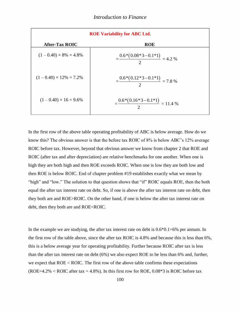
ROE Variability for ABC Ltd.

After-Tax ROIC ROE

(1 – 0.40) × 8% = 4.8% =

0.6* 0.08*3 0.1*1

2

= 4.2 %

(1 – 0.40) × 12% = 7.2% =

0.6* 0.12*3 0.1*1

2

= 7.8 %

(1 – 0.40) × 16 = 9.6% =

0.6* 0.16*3 0.1*1

2

= 11.4 %

In the first row of the above table operating profitability of ABC is below average. How do we

know this? The obvious answer is that the before tax ROIC of 8% is below ABC’s 12% average

ROIC before tax. However, beyond that obvious answer we know from chapter 2 that ROE and

ROIC (after tax and after depreciation) are relative benchmarks for one another. When one is

high they are both high and then ROE exceeds ROIC. When one is low they are both low and

then ROE is below ROIC. End of chapter problem #19 establishes exactly what we mean by

“high” and “low.” The solution to that question shows that “if” ROIC equals ROE, then the both

equal the after tax interest rate on debt. So, if one is above the after tax interest rate on debt, then

they both are and ROE>ROIC. On the other hand, if one is below the after tax interest rate on

debt, then they both are and ROE<ROIC.

In the example we are studying, the after tax interest rate on debt is 0.6*0.1=6% per annum. In

the first row of the table above, since the after tax ROIC is 4.8% and because this is less than 6%,

this is a below average year for operating profitability. Further because ROIC after tax is less

than the after tax interest rate on debt (6%) we also expect ROE to be less than 6% and, further,

we expect that ROE < ROIC. The first row of the above table confirms these expectations

(ROE=4.2% < ROIC after tax = 4.8%). In this first row for ROE, 0.08*3 is ROIC before tax

Corporate Dimensions of Risk

101

(EBITDA/IC) times IC which produces EBITDA (no depreciation in this problem). The term

0.1*1 is the $ interest payment on one million dollars of borrowing. The “2” in the denominator

is book-equity from the above invested capital balance sheet.

When the operating performance of ABC is below average (ROIC after-tax = 4.8%, which is less

than 6%), ABC shareholders do even worse. ROE is not only less than 6% but in addition ROE =

4.2% < ROIC after tax = 4.8%. This shortfall highlights the downside risk of debt use. When a

firms operating results are poor, shareholders do worse that the firm as a whole (the firm’s

performance for shareholders is ROE and the firm’s performance over-all is ROIC after tax and

after depreciation). Debt financing accentuates the adverse effect of below-average operating

performance of the business for shareholders. The “lows” are lower for shareholders compared

to the entire business.

On the other hand, if ABC’s operating performance is above average, it earns a 9.6% after-tax

ROIC. Since 9.6% exceeds 6% (the after tax interest rate on debt) the third row of results in the

above table is an above average year for ABC in their profitability. Further because 9.6% > 6%

we expect ROE to exceed 6% and, further, we expect ROE to exceed 9.6%. In this case, ABC

shareholders do even better that the firm as a whole, ROE > ROIC after-tax and after

depreciation (that is, 11.4% > 9.6%). This result highlights the upside potential of corporate debt

use for shareholders. Debt use accentuates above-average corporate operating performance for

shareholders. The “highs” are higher for shareholders compared to the entire business.

The middle row of results in the above table represents an average year for ABC in their

operating profitability. Even an average year for ABC is a relatively good year. How do we know

this? Because ROIC after tax and after deprecation is 7.2%, which exceeds 6%. Further because

7.2% > 6% we expect ROE to exceed 6% and, further, we expect ROE to exceed 7.2%. In this

case, ABC shareholders do better that the firm as a whole, ROE = 7.8 > ROIC = 7.2% (after-tax

and after depreciation). This comparison of business returns illustrates the average benefit of

Introduction to Finance

102

corporate debt financing for shareholders. As long as a business can invest at a before tax

business return (ROIC) that exceeds the interest rate on its debt, then average ROE will exceed

average ROIC. In our example, ROIC before tax = 12%, which exceeds the interest rate on debt.

In this case, the average ROE = 7.8% exceeds the average ROIC after tax = 7.2%. Shareholders

accrue the average benefit of corporate debt use. Of course, there are also risk “costs” to

shareholders, which we should also consider.

For shareholders, debt financing by the firm accentuates both the benefits of favorable operating

performance and the adverse consequences of unfavorable operating performance. One way to

measure the risk faced by the shareholders of ABC is with the range of ROE variability, 11.4% –

4.4% = 7.2%

3.5.1 ROE Variability and Debt Financing Title Page

Consider a hypothetical reorganization of the financial structure of ABC. Suppose that ABC

borrows another 1 million dollars with an annual interest rate of 10%. With the proceeds of this

sale, ABC buys back 1 million dollars of its common shares from shareholders. We presume the

change in the financial structure of ABC is presumed to take place with no impact on ABC’s

operating activities. In order words, ABC’s contribution margin, fixed cost, dollar sales, etc., are

all unaffected by financial structure. Let us refer to this new firm as DEF Ltd. DEF is identical

to ABC on its operating side, but DEF financed its operations with more debt than ABC. The

following table summarizes the invested-capital financing by DEF Ltd.

Invested Capital for DEF Ltd.

Debt = 2 million

Invested Capital = 3 million Equity = 1 million

Corporate Dimensions of Risk

103

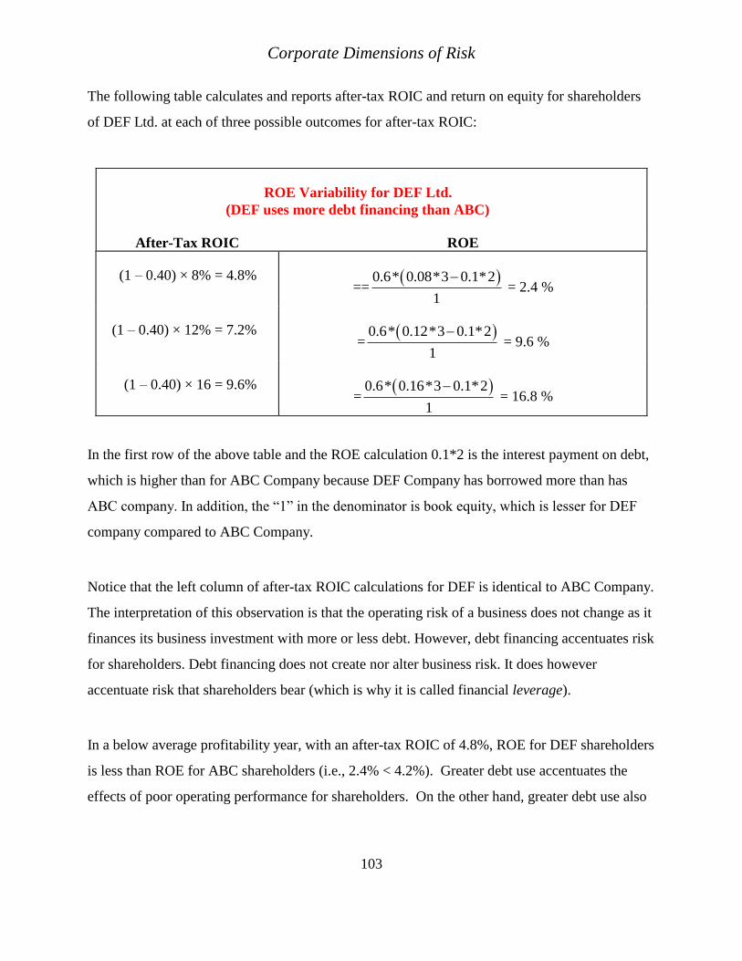
The following table calculates and reports after-tax ROIC and return on equity for shareholders

of DEF Ltd. at each of three possible outcomes for after-tax ROIC:

ROE Variability for DEF Ltd.

(DEF uses more debt financing than ABC)

After-Tax ROIC ROE

(1 – 0.40) × 8% = 4.8% ==

0.6* 0.08*3 0.1*2

1

= 2.4 %

(1 – 0.40) × 12% = 7.2% =

0.6* 0.12*3 0.1*2

1

= 9.6 %

(1 – 0.40) × 16 = 9.6% =

0.6* 0.16*3 0.1*2

1

= 16.8 %

In the first row of the above table and the ROE calculation 0.1*2 is the interest payment on debt,

which is higher than for ABC Company because DEF Company has borrowed more than has

ABC company. In addition, the “1” in the denominator is book equity, which is lesser for DEF

company compared to ABC Company.

Notice that the left column of after-tax ROIC calculations for DEF is identical to ABC Company.

The interpretation of this observation is that the operating risk of a business does not change as it

finances its business investment with more or less debt. However, debt financing accentuates risk

for shareholders. Debt financing does not create nor alter business risk. It does however

accentuate risk that shareholders bear (which is why it is called financial leverage).

In a below average profitability year, with an after-tax ROIC of 4.8%, ROE for DEF shareholders

is less than ROE for ABC shareholders (i.e., 2.4% < 4.2%). Greater debt use accentuates the

effects of poor operating performance for shareholders. On the other hand, greater debt use also

Introduction to Finance

104

accentuates good operating performance. At a 9.6% after-tax ROIC, ROE for DEF shareholders

is greater than ROE for ABC shareholders (i.e., 16.8% > 11.4%).

We can measure the additional risk that shareholders of DEF bear compared to shareholders of

ABC with the range of ROE. For DEF Ltd., the range of ROE is 14.4% (16.8% - 2.4%). This

range is greater than 7.2%, the ROE range for ABC Ltd (11.4% - 7.2%). This example illustrates

that debt use by a firm increases risk which shareholders bear.

The fact that debt imposes incremental risk on shareholders does not imply that firms should

avoid debt. Debt use also confers advantages on shareholders. One of these advantages is that, as

long as the average pre-tax ROIC exceeds the cost of debt, shareholders earn a higher average

rate of return as a consequence of debt financing. For example, average ROE's for shareholders

of ABC and DEF are 7.8% and 9.6% respectively. The shareholders of DEF bear additional risk

but they also earn a higher average rate of return on their investment.

Second, there are tax advantages of debt use. ABC’s average yearly tax bill is

(0.40)×[(0.12)×$3m – (0.10)×$1m] = $104,000. On the other hand, DEF’s tax bill is

(0.40)×[(0.12)×$3m – (0.10)×$2m] = $64,000. DEF has a lesser tax bill because debt increases

the tax deductions a profitable firm may claim.

In sum, the use of debt financing increases risk, but it can also increase expected return.

Depending on the economic environment, each firm may find net gains in value by either

substituting debt financing for equity, or by substituting equity financing for debt. It is possible

that, in some economic environments, the risk disadvantage of debt use is exactly offset by the

return advantage of debt use.

Corporate Dimensions of Risk

105

(3.6) Summary Title Page

There are two fundamental determinants of the investment risk faced by shareholders of a firm.

The first we refer to as operating leverage. Operating leverage measures the percentage change

in EBITDA for each one-percent change in Sales. All else equal, shareholders face greater risk if

they invest in firms with higher operating leverage. Important determinants of a firm’s operating

leverage are contribution margin per sales dollar, fixed costs, and $SALES. Greater contribution

margin decreases operating leverage. Greater fixed costs increase operating leverage. Greater

$SALES decrease operating leverage.

Firms have only modest influence over their operating leverage. Cost reductions and revenue

increases reduce operating leverage, but oftentimes, these factors are determined by the economic

environment and not at managers’ discretion.

Firms have more discretion in the choice of financial leverage. Debt financing increases the risk

of shareholders’ returns. Nonetheless, if a firm can invest in real assets to earn an average before-

tax ROIC that exceeds the interest rate on debt, greater debt use increases average ROE. Greater

expected ROE is an advantage of using additional debt.

Introduction to Finance

106

(3.7) Suggested Reading Title Page

George W. Blazenko, Freda Eddy-Sumeke, and Yufen Fu. “Business Profit and Consumer Price

Sensitivity.” Journal of Business and Economic Management, Vol 2, No. 6, (2014), 84-96.

George W. Blazenko, "Corporate Leverage and the Distribution of Equity Returns," Journal of

Business Finance and Accounting Vol. 23, (1996), 1097-1120.

Yufen Fu and George W. Blazenko. “Returns for Dividend Paying and Non-Dividend Paying

Firms.” International Journal of Business and Finance Research, Vol. 9, No. 2, (2015), 1-15

(lead article).

Lerner AP (1934). The concept of monopoly and the measurement of monopoly power. Rev.

Econ. Stud. 1(3):157-175.

Moisescu OI, Allen B (2010). The relationship between dimensions of brand loyalty: an

empirical investigation among Romanian urban consumers. Manage. & Marketing Challenges

for the Know. Soc. 5(4):83-98.

Corporate Dimensions of Risk

107

(3.8) Problems

1. DOL, Break-even Sales, and EBITDA Margin. For the fiscal year 2000, ABC had a degree

of operating leverage of 1.5 and a net operating margin of 20%. For 2000 break-even dollar

sales was $1,200,000. What was ABC’s EBITDA? What were ABC’s dollar sales for

2000?

Title Page

Solution

2. DOL, ROIC, ROE. ABC Company has a contribution-margin per dollar sales of 20%.

Fixed costs are $30,000 per annum. ABC has invested capital of $3,000,000. Trade capital

and net fixed assets represent 60% and 40% of invested capital respectively. Invested

capital has been financed with $1,200,000 in short-term debt and $1,800,000 in equity. The

interest rate on short-term debt is 10% per annum. ABC’s tax rate is 23%. Depreciation,

which is also equal to capital cost allowance, is 5% of beginning-of-period net fixed assets.

a) What is the degree of operating leverage at break-even sales?

b) Does the degree of operating leverage increase or decrease with dollar sales? Explain.

c) Find the level of dollar sales for the upcoming year such that ROIC after tax and after

depreciation is equal to ROE. Use beginning of period invested capital and equity for

ROIC and ROE respectively.

Title Page

Solution

3. DOL and Break-even Sales. If break even sales increases (in either dollars or units),

operating leverage has also increased. Discuss and comment on this assertion.

Title Page

Solution

Introduction to Finance

108

4. Corporate Debt Use. Comment on the following assertion. “Firms should not use debt to

finance their business activity because it imposes additional risk on shareholders.”

Title Page

Solution

5. DOL, EBITDA-margin. ABC Company has a contribution margin per dollar sales of 32%

and an EBITDA margin of 20%. What is ABC’s degree of operating leverage?

Title Page

Solution

6. DOL, ROIC, and ROE. ABC Company has a tax rate of 40%. Their invested capital is

$3,000,000. This investment is financed with short-term debt and with equity. Their debt to

equity ratio is 2.0. “Equity” represents all of the accounting equity accounts. The interest

rate on ABC’s short-term debt is 6% per annum. ABC has a contribution margin per dollar

sales of 32%. In the upcoming year, ABC’s dollar sales are predicted to be $2,400,000.

Also in the upcoming year, depreciation on ABC’s fixed assets will be $200,000. Based on

these predictions, ABC expects that in the upcoming year, their rate of return on invested

capital (after tax and after depreciation) will be equal to their rate of return on equity. Both

the rate of return on invested capital and the rate of return on equity are calculated as

“beginning of period” with respect to the prediction year.

Required: Based on the given information, find ABC’s degree of operating leverage for the

upcoming year (based on predicted sales).

Title Page

Solution

7. DOL, ROIC, and ROE. ABC Company has a tax rate of 40%. Invested capital is

$3,000,000. This investment is financed with short-term debt and with equity. Currently,

ABC is financed with $1,500,000 of short-term debt and with $1,500,000 of equity. Equity is

the sum of retained earnings and share-capital. ABC’s trade-capital to invested capital ratio

Corporate Dimensions of Risk

109

is 55%. The interest rate on ABC’s short-term debt is 7% per annum. In the upcoming year,

at predicted sales of $2,760,000, ABC’s rate of return on invested-capital (after tax and after

depreciation) is equal to its rate of return on equity. Both the rate of return on invested

capital and the rate of return on equity are calculated as “beginning of period” with respect to

the prediction year. Fixed operating costs in the upcoming year are expected to be $207,000.

Also, in the upcoming year, depreciation on ABC’s net fixed assets (which is the same as

CCA) will be 10% of the opening balance. No capital expenditures or asset sales are

expected in the prediction year. Also, none of ABC’s short-term debt will be paid down over

the upcoming year.

Required: Find ABC’s predicted degree of operating leverage for the upcoming year.

Title Page

Solution

8. Financial Leverage

Comment on the following assertion: “Because of financial leverage, the rate of return on

equity (ROE) for a firm in a particular year is always greater than its rate of return on

invested capital (ROIC, after tax and after depreciation).” Use no numerical examples in

your response.

Title Page

Solution

9. DOL.

At dollar sales of $4,000,000, ABC Company Limited has an EBITDA-margin of 20%. Their

break-even dollar sales for a year are $2,000,000. Break-even sales are defined as dollars sales

for which EBITDA (from core operations) is zero.

Required: What is ABC’s Degree of Operating Leverage at sales of $3,000,000?

Title Page

Solution

Introduction to Finance

110

10. DOL.

ABC Company has a contribution-margin per dollar sales of 25%. Fixed operating costs

(before tax, depreciation, and interest) are $300,000. ABC has invested capital of

$4,000,000. Trade capital and net fixed assets are 34% and 66% of invested capital

respectively. Invested capital has been financed with $1,200,000 in short-term debt and

$2,800,000 in equity. The interest rate on short-term debt is 10% per annum. ABC’s tax rate

is 40%. Depreciation, which is also equal to capital cost allowance, is 5% of beginning-of-

period net fixed assets. Other things equal, ABC’s predicted rate of return on invested capital

after tax and after depreciation for the upcoming year (using beginning of period invested

capital) is 24%.

Required: What is ABC’s degree of operating leverage at predicted dollar sales?

Title Page

Solution

11. DOL.

Comment on the following assertion. “A principal determinant of the Degree of Operating

Leverage (DOL) is corporate debt use.” Use no numerical examples in your response. A

complete response is required for full marks.

Title Page

Solution

12. DOL

ABC Company Ltd. has a contribution margin per dollar of sales of 25%. Their degree of

operating leverage (DOL) is 1.25 when dollar sales are $2,000,000 per annum.

Required: Find ABC’s break-even annual dollar sales (break-even in terms of EBITDA).

Title Page

Solution

Corporate Dimensions of Risk

111

13. ROIC and Corporate Debt Use.

Comment on the following assertion. “A primary determinant of a firm’s rate of return on

invested capital (after tax and after depreciation) is corporate debt use.” Use no numerical

examples in your response. A complete response is required for full marks.

Title Page

Solution

14. DOL

ABC Company Ltd. has fixed operating costs of $200,000 per annum. Their degree of operating

leverage (DOL) is 1.25 when dollar sales are $2,000,000 per annum.

Required: Find ABC’s annual dollar sales that break-even in terms of EBITDA.

Title Page

Solution

15. DOL.

Comment on the following assertion. “Because a firm’s EBITDA margin is before fixed

operating costs, whereas, contribution margin per dollar sales is after fixed operating costs,

EBITDA margin exceeds contribution margin per dollar sales, and therefore, the degree of

operating leverage (DOL), which is contribution margin per dollar sales divided by EBITDA

margin, must be lesser than or equal one.” State whether you agree or disagree with the assertion

and if so, why, and if not, why not. Discuss the aspects of the assertion that you agree with and

those that you do not agree with. Use no numerical examples in your response. A complete

response is required for full marks.

Title Page

Solution

Introduction to Finance

112

16. DOL

ABC Limited has a degree of operating leverage (DOL) of 1.25 when dollar sales are $2,000,000

per annum.

Required: Find ABC’s annual dollar sales that break-even in terms of EBITDA. Recall that

break-even dollar sales are fixed operating costs divided by contribution margin per dollar sales.

You need not determine these amounts separately, but only their ratio.

Title Page

Solution

17. Financial Leverage.

Comment on the following assertion. “When a firm does well on its business investments, that

is, EBITDA is high, the rate of return on invested capital (ROIC) is correspondingly high and

exceeds the rate of return on equity (ROE). On the other hand, when a firm does poorly on its

business investments, ROIC is low and is below ROE.” State whether or not you agree with the

assertion and then explain why. Use no numerical examples in your response. A complete

response is required for full marks.

Title Page

Solution

18. DOL and ROIC.

If ABC Company’s per annum sales equal $4,000,000, then their EBITDA margin is 20% and

their degree of operating leverage (DOL) is 1.5. On the other hand, if ABC’s ROIC (rate of

return on invested capital after tax and after depreciation with end of period invested capital)

equals their ROE (rate of return on equity with end of period book equity) then, dollar sales equal

$3,000,000 per annum. ABC pays interest on their debt at the rate of 8% per annum. ABC’s

corporate tax rate is 40%. ABC’s depreciation expense is $300,000 per annum.

Required: Find the dollar amount of ABC’s end of period invested capital.

Title Page

Solution

Corporate Dimensions of Risk

113

19. A Benchmark for ROIC and ROE

ABC Company has debt and common equity in its financial structure. The interest rate on ABC

Company’s debt is 10% per annum. The corporate tax rate is 40%. In 2006, ABC’s ROIC (after

tax and after depreciation) equals ROE. For 2006 what was ABC’s ROIC?

Title Page

Solution

20. EBITDA Increases with $SALES

ABC Company Ltd. has a contribution margin per dollar sales of 20% and fixed annual operating

costs of $1,000,000. If ABC’s EBITDA margin is 15%, what are dollar sales? Given the same

assumed facts, but the EBITDA margin is 18%, what are dollar sales (other things equal).

Title Page

Solution

Introduction to Finance

114

(3.9) Chapter Index Title Page

break-even, 90

capital structure, 99

coefficient of determination, 93

contribution margin, 91, 92

Contribution margin, 82, 90

degree of operating leverage, 85, 91

dependent variable, 93

EBITDA margin, 86, 89

financial leverage, 81, 105

financial structure, 99

fixed costs, 90

independent variable, 93

invested capital, 81, 99

operating efficiency, 88

operating leverage, 81

operating risk, 89

Operating risk, 85

rate of return on equity, 81

rate of return on invested capital, 81

revenue-based risk, 93

risk, 81

simple linear regression, 92

variable costs, 89