chapter 3: basic probability and statistics - calvin … · chapter 3: review of basic probability...
TRANSCRIPT
Chapter 3: Review of Basic Probability and Statistics: Part One
0.a Context 1: Read On You have already completed a semester of calculus and a semester of college statistics, so this chapter and
the next should largely be a review for you. But, just to be sure we are all on the same page, please don’t
skip anything. Don’t even read fast.
After the last page of text you will find some practice problems, then a brief review of STATA commands
that you’ll find useful for some of these problems, then a set of statistical tables that can be used at times
when you lack access to STATA.
0.b Context 2: Getting to Know our Ignorance We might say that there are two kinds of statistical work, each trying to fix a different kind of ignorance.
This chapter and the next discuss each type separately.
1. Statistics Part One: Population familiar, sample unfamiliar Say that we know something about the whole population of things under discussion, and we’re trying to
draw an deduction about what might be true of a smaller sample from this population. This leads to classic
statistics questions like:
A computer hard drive manufacturer produces drives whose lifespan until crashing is normally
distributed, with a mean of three years and standard deviation of six months. Find a warranty
period that will result in a 5% return rate for the drives.
or
A pair of fair dice has been rolled four times, and each time the dots showing have summed to
seven. What is the probability that the next toss returns a sum of seven?
See there? In each case we knew something about the whole universe (the pattern that describes failures of
hard drives, or the number of spots on each side of a die and the fact that each side is equally likely for fair
dice). Then we were asked to characterize a typical (that is, truly random) but as-yet unknown small
sample from that universe.
The truly amazing thing is that, though the samples are completely random and therefore unknowable in
advance, the characteristics of these samples follow patterns, and those patterns are governed in part by the
population’s characteristics. This makes it possible to anticipate things that should by nature be
unknowable. Why should failures of hard drives follow any pattern at all, and why should this pattern be
completely determined if you just know its mean and standard deviation, and why should this pattern be so
common among so many completely different things that we call it the ―normal‖ pattern? A universe
constructed without these discernable, predictable patterns would make modern complex civilization
extremely difficult. Like the other features of our universe that biochemistry professor Michael Behe has
discussed in Darwin’s Black Box, this is either evidence of intelligent design or a series of incredible
happenstances. To a naturally skeptical person like me, the happenstantial explanation seems gullible and
sentimental.
2. Statistics One: The Fundamental Words
As in sailing or playing bridge, you need some short phrases with precise definitions if you want to proceed
in bearably good time. One way to review your stats course is to reiterate the core definitions from that
course. Here are some of the most important, arranged logically (from population to sample to deduction)
rather than alphabetically. You’ll remember them better if you jot down a summary as you read:
Population Parameter: A characteristic of the whole population (like the average lifespan in the
whole population of hard drives). Greek letters are usually used as symbols for population parameters:
The population mean is usually called ―mu‖ ( ), the standard deviation ―sigma‖ ( ), the slope of a
function linking two variables ―beta‖ ( ), and so forth.
Random sample: A sample with size N is a random sample if every combination of N elements in the
population has an equal chance of being selected. There are other ways of sampling from a population,
but we will concentrate on random sampling in this course.
Random (or “Stochastic”) Variable: The measure of a characteristic of a sample drawn from the
population (like the lifespan of a particular randomly-drawn hard drive). Notice that population
parameters (mentioned above) aren’t random; they’re fixed, an objective reality that’s independent of
the researcher’s point of view. It’s random samples from populations that yield random variables—
which are ―random‖ measurements because each sample will probably be a little different from the
last. By convention, random variables are often referred to as ―X,‖ the Greek ―chi,‖ when we’re
talking about a whole population of them, and x, the Roman ―eks,‖ when referring to a particular
observation. Random variables come in two flavors:
Continuous random variables: These are measures of characteristics that, ... well, vary
continuously. It’s conceivable that the measurement in one sample is very, very close to the
measurement in another sample, yet still different from it. One hard drive might last 3.45678
years, and the next sample could last 3.45679 years. ―Hard drive lifespan‖ is a continuous
random variable.
Discrete random variables: These are measures of characteristics that change in ―discrete‖ jumps,
with some never-observed space between each possibility. When you roll a die, it never comes up
showing 3.24 dots; ―number of dots showing‖ is a discrete random variable.
Of course, if you add together the lifespan of three randomly-drawn hard drives and then divide by three,
the result is often called a ―random variable‖ too, though technically it is better termed a...
Statistic: A number that is computed from sample measurements of individual random variables,
without knowledge of any of the population parameters. In other words, a statistic is a number that
results from inserting some sample data into a formula—like sample means, sample standard
deviations, and so forth. You might try reading ―formula‖ each time you see the word ―statistic.‖ A
statistic measures some characteristic of a sample.
Sample characteristics are usually referred to by Roman letters (though we’ll encounter an exception
two chapters from now). This distinguishes them from the population’s parameters (Greek letters).
We’ll normally use italic Roman letters, to set them off from the rest of the text. Thus a sample
standard deviation may be called s (whereas the standard deviation within the whole population would
be ), a sample slope would be b, and so forth. Remember: Greek for population parameters, Roman
for sample measurements. The Greeks came before the Romans, and you need a population before you
can take samples.
One very annoying exception we can handle right now: A sample mean is often noted as
_
x (read ―x
bar‖) rather than m (which would correspond to the population parameter ). This probably happened
because we were calling the random variable , and many people instinctively think of m as a
population slope (from the Standard Equation Of A Line, y=mx + b), rather than a sample
characteristic. Now note with sadness one more bizarre twist: In statistics we are using the Roman b
to refer to a sample’s calculated slope, while algebra’s standard equation uses b to refer to the
intercept, not the slope. Here is a little Rosetta Stone to clarify things:
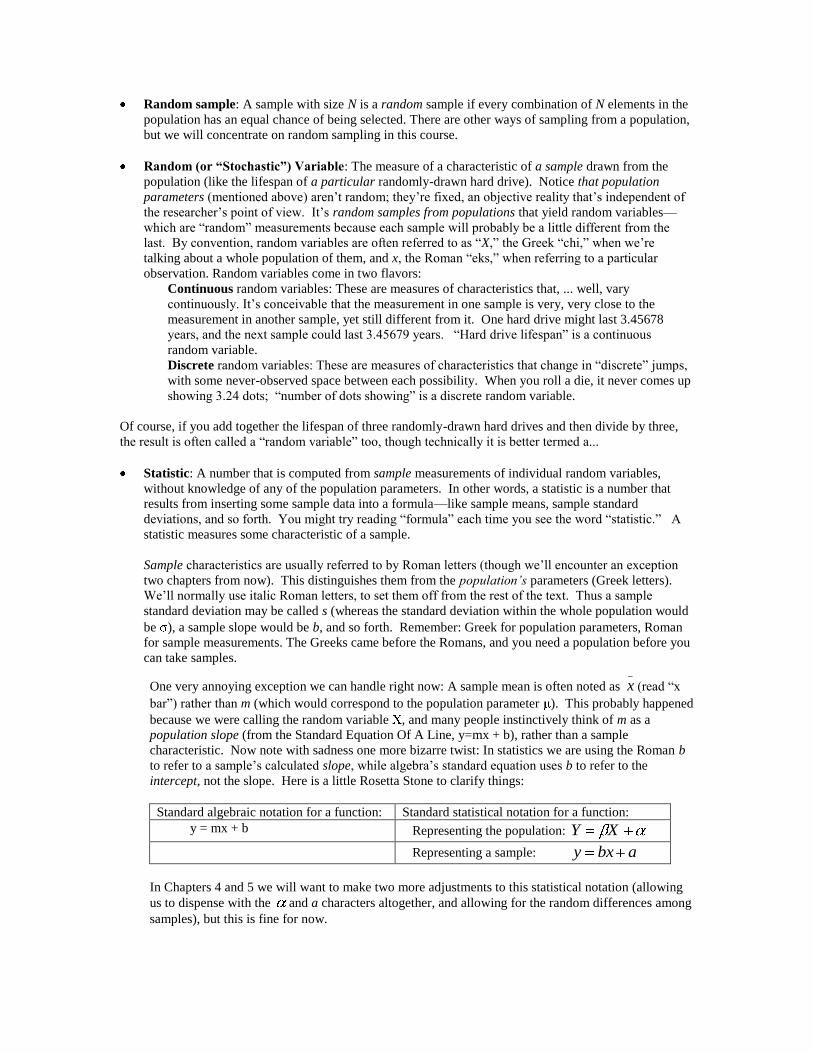
Standard algebraic notation for a function: Standard statistical notation for a function:
y = mx + b Representing the population: XY
Representing a sample: abxy
In Chapters 4 and 5 we will want to make two more adjustments to this statistical notation (allowing
us to dispense with the and a characters altogether, and allowing for the random differences among
samples), but this is fine for now.
Just to drive home the difference between population parameters and sample statistics: Notice that, in
our hard drive problem, ―three years‖ and ―six months‖ refer to population parameters, not statistics.
These numbers tell you something about the universe of hard drives before you ever draw a sample or
compute a statistic from that sample.
Sample Statistic: That’s redundant, isn’t it? ―Statistics‖ only come from samples, without reference to
the whole population. But for reinforcement we often use this phrase to refer to sample attributes that
have been measured and combined (via a formula) into a statistic. When you simultaneously roll two
dice and sum the dots, you’re calculating a sample statistic; when you average the number of dots from
the last three rolls, that’s another sample statistic.
Sample Size: The number of observations upon which your sample statistic is based. If you compute
the average lifespan of three hard drives, your sample size is three. In our dice-rolling problem, when
you simultaneously roll two dice and sum the dots, the sample size is equal to one. (Did you think it
would be two? Remember that the thing we are observing is ―the sum of dots on two simultaneously
rolled dice,‖ and we have observed that thing only once.) When you average the number of dots from
the last three rolls, the sample size is three. By convention, sample size in any particular problem is
usually noted by a Roman N.
Degrees of Freedom: This is one measure of how much information our sample contains. Texts
seldom actually define the concept, but here is an attempt:
Say you know that the average of two hard drives’ lifespans was 1.5 years, and you also know that
one of these hard drives lasted 2 years. Then you actually already know how long the second hard
drive lived, without directly measuring it. One observation is ―determined‖ by the other two
things you know; it is no longer free to vary. Now reverse the logic: If you have two observations
and then compute from them an average, it’s as if the computation has ―used up‖ the information
in one of your observations. Computing a sample average is ―expensive‖ in that, once we do it, we
have less free information left to manipulate—one less observation, to be precise. So you might
say we have lost one ―degree of freedom‖ by calculating an average, and now have N-1 degrees of
freedom left. Though we had N independent pieces of information, we only have N-1 independent
deviations from the sample mean.
We will often be concerned about how many degrees of freedom exist in a sample, because our ability
to learn from the sample depends upon how much information the sample contains.
Probability Distribution: The pattern that a population or particular random variable or sample
statistic tends to follow. You might try reading ―pattern‖ each time you see ―probability distribution.‖
This is sometimes called a ―density function.‖ since it tells us which outcomes tend to be distributed
sparsely (not observed frequently) and which others are observed frequently (with more density). We
will often note the probability density function of random variable X as fX(X) or, wherever
simplification won’t lead to confusion, f(X). Sometimes it will be easier to refer to the probability of a
particular x as simply Pr(x).
Notice a subtle idea in that last definition: If individual observations of a random variable follow a pattern,
say a normal distribution, then combinations of these individual observations (sample statistics) usually
also follow some predictable pattern.
i.i.d. variables: A truly random sample of N observations of the random variable X has a pleasant
property: We are left with N ―i.i.d stochastic variables‖ (for ―identically, independently distributed‖),
each following the same probability distribution. This property will make our task much simpler in the
chapters that follow.
3.a Moments of Probability Distributions: One Single Random Variable We just said that a probability distribution is a pattern that a random variable tends to follow—a summary
of its behavior. It is sometimes useful to further summarize these patterns with a number or two, and the
most useful summary numbers are ―moments.‖ Here the word is used not in the chronological sense (as in
―just a moment, please...‖) but in its Latin-root sense (momentum, momentous)—a reference to force and
weight. Moments of distributions give us a simple summary measure of where the ―weight‖ in the
distribution lies: which observations are most typical (that is, centers of weightiness), how diverse the
observations tend to be (that is, how spread-out the weight of the distribution is), and so forth.
Here are four useful moments of probability distributions:
The Mean: The most common measure of the ―central tendency‖ of a population or sample—an
attempt to summarize the typical value of a random variable.
For populations, we could define the mean of a probability distribution as the expected value of X , or
mathematical expectation of X , usually noted as either (―mu‖) or E(X) (read ―expected value of X‖).
This is a weighted average of all the possible values of X, where the weights are the probabilities of
observing each value. Recall that every random variable will have a mean, but the mean of a
population is not a random variable; it’s a constant, a population parameter, a property of the
population that does not vary.
For a discrete random variable, we could write the population weighted-average E(X) as
)()(1
i
i
i xfxXE , 3.1
where (that’s a capital nu, since we’re talking about a population) is the number of possible
outcomes and f(x) is the probability function. (For a continuous variable, we’d have an integral instead
of a summation symbol.)
This equation implies that E(X) is the first moment around the origin, yet another synonym for the
mean. The second moment around the origin would be )()(1
2
i
i
i xfxXE --―first‖ and ―second‖ refer
to the power to which the random variable is raised, before finding a weighted average. We call this a
moment ―around the origin‖ because we are subtracting zero—the origin—from X before raising it to a
power and then computing a weighted average. Thus we could take, say, a seventh moment around
nine,
)()9()(
7
1
i
i
i xfxXE , if we felt like it.
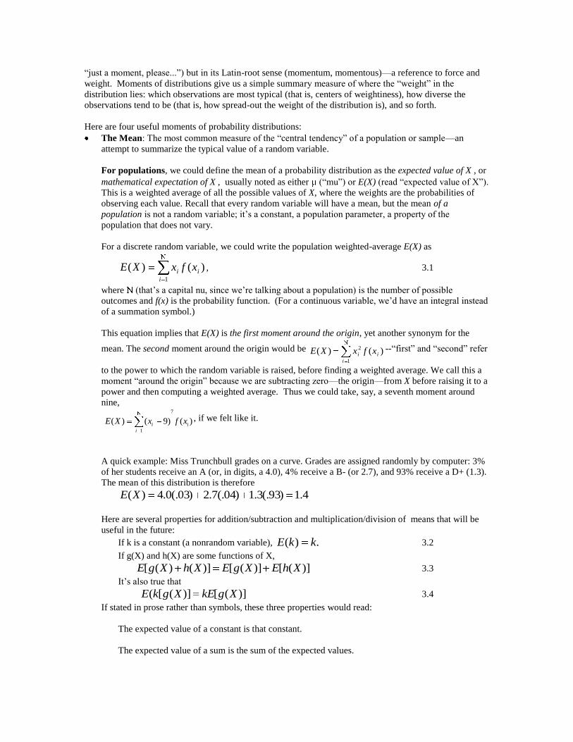
A quick example: Miss Trunchbull grades on a curve. Grades are assigned randomly by computer: 3%
of her students receive an A (or, in digits, a 4.0), 4% receive a B- (or 2.7), and 93% receive a D+ (1.3).
The mean of this distribution is therefore
4.1)93(.3.1)04(.7.2)03(.0.4)(XE
Here are several properties for addition/subtraction and multiplication/division of means that will be
useful in the future:
If k is a constant (a nonrandom variable), .)( kkE 3.2
If g(X) and h(X) are some functions of X,
)]([)]([)]()([ XhEXgEXhXgE 3.3
It’s also true that
)]([)]([( XgkEXgkE 3.4
If stated in prose rather than symbols, these three properties would read:
The expected value of a constant is that constant.
The expected value of a sum is the sum of the expected values.
Constants can be factored out of expected value computations.
Taken together, these three properties imply that
0)(XE . 3.5
Here ends our discussion of the population mean.
For samples, the sample mean (which, you’ll recognize, is a sample statistic, whereas the population
mean is a population parameter) is simply the average of the random variables that were observed,
usually noted as
NxxN
i
i /][1
. 3.6
Unlike the population mean, the sample mean is a random variable, since the computed average will
generally be a bit different for each sample.
A quick example: Matilda has taken three classes with Miss Trunchbull. Her grades have been B-, B-
and D+. Her mean grade is
23.23/]3.17.27.2[x .
Notice that the sample mean doesn’t necessarily equal the population mean.
The Variance and Standard Deviaion: These are the most common measures of the variability (or
―dispersion‖) of a random variable around its central/typical value. They attempt to summarize the
diversity within a group.
For populations, variance and standard deviation add up the variability within a population this way:
(X- ) measures how different each instance of a variable is from the ―typical‖ value
Squaring this measure, (X- )2, converts negative deviations into positive ones, so we can add
them all up without having some cancel out others.
Finding the expected value of this squared deviation gives us a typical squared deviation—
one measure of how much X varies around its mean:
])[()( 22 XEXVar X . 3.7
This is the variance, or second moment of X around its mean. (People sometimes write
Var(X) rather than 2
X because it’s easier to type and easier to read when you’re finding
the variance of a long equation.)
Since this is the typical squared deviation around the mean, you’d get a measure of
the typical deviation by finding the square root of the variance—the so-called
―standard deviation:‖
2)( XXXSD . 3.8
For discrete random variables, you’d find the expected value in equation 3.7 by calculating
)()( 2
1
i
i
i xfx . 3.9
Continuous random variables would require an integral rather than a summation.
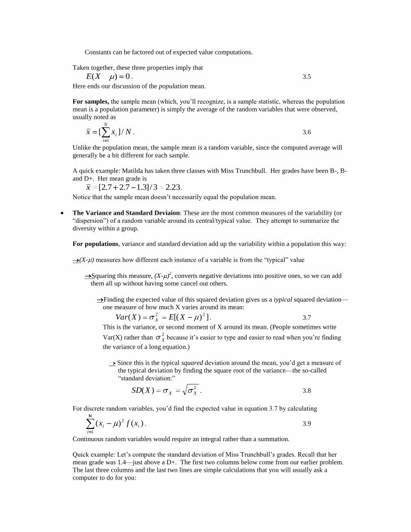
Quick example: Let’s compute the standard deviation of Miss Trunchbull’s grades. Recall that her
mean grade was 1.4—just above a D+. The first two columns below come from our earlier problem.
The last three columns and the last two lines are simple calculations that you will usually ask a
computer to do for you:
ix )( ixf ix 2)( ix )()( 2
ii xfx
4.0 .03 2.6 6.76 0.2028
2.7 .04 1.3 1.69 0.0676
1.3 .93 -0.1 0.01 0.0093
)()( 2
1
i
i
i xfx = 0.2797
)()( 2
1
i
i
i xfx = 0.5289
Interpretation of standard deviation in prose: On a four-point grading scale, Miss Trunchbull’s
―typical‖ (mean) grade is 1.4, but not all of the grades are stacked up exactly at 1.4; the ―typical‖
spread (standard deviation) from the mean to any one grade is 0.5289, just over half a letter grade.
Variance and standard deviation might not deserve their celebrity status. You could think of other
ways to measure diversity within a population--like adding up absolute-value deviations rather than
squared deviations, so you wouldn’t exaggerate extreme values. And, since the standard deviation
measures deviations around the mean, it is a meaningless measure of diversity if the distribution has no
clear central tendency. I mean, what would be the ―typical‖ deviation from mean height in a room
filled with professional basketball players and professional jockeys? Yet variance and standard
deviation have become common measures of dispersion because, as we will see, they are often more
powerful and easier to manipulate mathematically than other options.
Just as with the population mean, there are several propertes of the population variance that will be
useful in the future:
])[( 22 XEX can, by completing the square and collecting terms, be written as
2222 )(])[( XEXEX . 3.10
02
k when k is any constant. 3.11
)()( 2 XVarkkXVar 3.12
In prose:
The population variance equals the expected value of X-squared, minus the expected value of X,
squared. (!)
The variance of a constant is zero. (Constants don’t vary!)
If you multiply a variable by k, its variance increases k2-fold.
These three properties cover basic multiplication/division for population variances. We can’t explore
properties of addition/subtraction until our discussion of covariance in Section 3b.
For samples, the sample variance (which is a sample statistic, of course) is a measure of the dispersion
within the sample, calculated as
2
1
2 )(1
1xx
Ns
N
i
i . 3.13
(The sample standard deviation, s, is simply the square root of s2.) Notice the denominator: You’d
expect to compute this typical squared deviation by dividing by N rather than N-1. But recall:
You have to compute a sample mean before you can compute the variance around that mean,
and
computing a sample mean ―uses up‖ the information in one observation (remember the discussion
about ―degrees of freedom‖ in section 2?).
Therefore we only have N-1 degrees of freedom left when we compute the sample variance. Now
imagine that our sample consisted of the entire population. If we computed the sample variance by
dividing by N rather than N-1, it turns out that the expected value of our sample variance statistic
would no longer equal the population variance, which would make it an unreliable statistic indeed. We
can avoid this bias by simply dividing the sum of squared deviations of X by the number of degrees of
freedom, N-1.
Quick example: Pause now to compute the standard deviation of Matilda’s grades. You should get
65335.0 =0.808. Again, the sample standard deviation is not necessarily equal to the population
standard deviation.
The Coefficient of Variation: We should briefly mention this population parameter, defined as the
ratio / . This measures the dispersion within a population relative to the population mean.
Imagine that you’re a quality-control officer for a ball-bearing manufacturer. You might be more
concerned about a 0.01mm standard deviation among your 0.1mm bearings than the same-sized
variation among your 5000mm bearings, because smaller bearings probably have to meet more precise
tolerances. Tolerances are probably stated as a percentage of the bearing size. If so, the coefficient of
variation is one way of standardizing the dispersion within populations when those populations have
different means.
3.b Moments of Probability Distributions: More Than One Random Variable Of course the whole probability distribution of a random variable could be altered by changes in a different
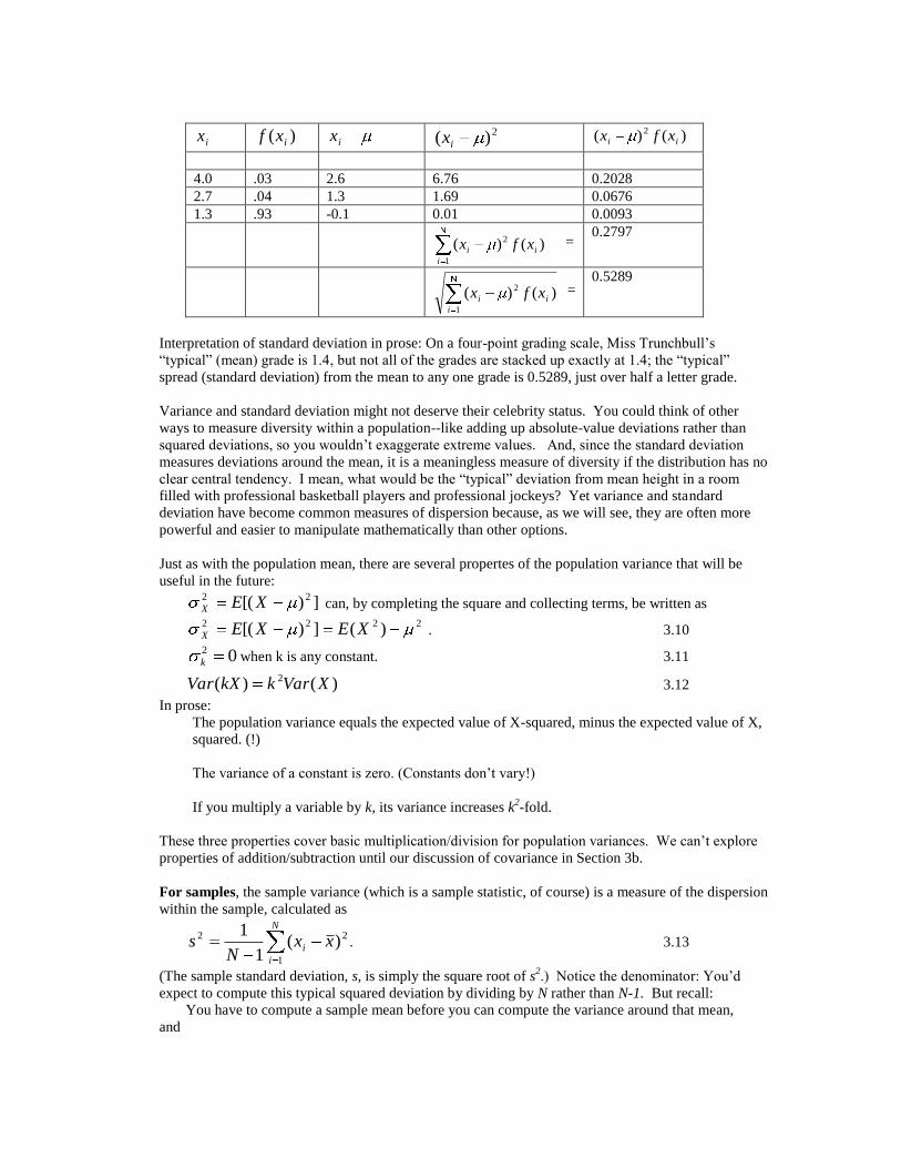
variable. For example, say that the number of math courses completed in college (we’ll call this variable X)
affects the probability distribution of the number of job offers (we’ll call this variable Y) received by senior
Econ majors from Whatsamatta U, in the following way:
Math courses completed 2 3 4
Job offers Joint probabilities: fXY(x,y)
1 0.05 0.03 0.02
2 0.10 0.05 0.02
3 0.10 0.15 0.02
4 0.05 0.05 0.10
5 0.01 0.05 0.20
When a probability distribution of one variable is influenced by a different variable, we have a joint
probability distribution, in this case a discrete (not continuous) bivariate (two-variable) joint probability
distribution. Here, for example, the probability that one receives four job offers after taking only two math
courses is equal to 0.05, or, in symbols,
05.0)4,2Pr( ,
or, equivalently,
05.0)4,2(XYf .
As with any good probability distribution, the probabilities of the fifteen possibilities sum to 1.0, which
means that all econ majors at this school take 2, 3 or 4 math courses, and receive 1, 2, 3, 4 or 5 offers.
We could augment this probability distribution by computing the marginal probabilities, the probability
that X or Y takes on any particular value regardless of the value of the other variable, by summing across
the rows, then across the columns, while putting the results in the margins:
Math courses completed 2 3 4
Job offers Joint probabilities: fXY(x,y) Marginal Pr(Y): h(Y)
1 0.05 0.03 0.02 0.10
2 0.10 0.05 0.02 0.17
3 0.10 0.15 0.02 0.27
4 0.05 0.05 0.10 0.20
5 0.01 0.05 0.20 0.26
Marginal Pr(X): g(X) 0.31 0.33 0.36 x y
YX 1)Pr()Pr(
In prose: The probability that a senior receives, say, four offers, ignoring the number of math courses taken,
is 0.20; the marginal probability of taking three math courses is 0.33. Notice that the marginal
probabilities for each variable also sum to 1.00.
Having defined the population’s joint and marginal density functions, let’s review some useful results
about the population parameters of jointly-distributed variables:
Independence: The random variables X and Y are statistically independent if their joint probability is
equal to the product of their marginal probabilities:
)()(),( YhXgyxf XY . 3.14
In prose: Two variables are not independent if the level of one influences the probability distribution of
the other; we can check by multiplying marginal probabilities.
Expected value: Let ),( YXw be any function involving the random variables X and/or Y, and let
),( yxf XY be the joint probability distribution of the variables. Then the expected value of
),( YXw is given by
Y
XY
X
yxfyxwYXwE ),(),()],([ 3.15
for discrete variables. (We’d use integrals rather than summations for continuous variables.)
In prose: The expected value (that is, mean) of a function of jointly-distributed variables is a weighted
average of the function’s values, where the weights are the joint probabilities.
A quick example: To find the expected value of the number of job offers at Whatsamatta U, our
),( YXw is simply equal to Y (that’s the number of offers, right?), so working across all the rows of
the original table we have
20.0505.0210.0202.0103.0105.01),()],([ Y
XY
X
yxfyYXwE
= 3.35.
Variance: Nothing new here. The variances of the random variables X and Y are simply
])[( 22
XX XE and ])[( 22
YY YE ,
where the i are expected values.
Covariance: We often want know if one variable systematically rises or falls as the other variable
changes, and covariance is one way of deciding. Imagine that one variable (say, the number of job
offers, Y) tends to rise as the other variable (number of math courses, X) increases. When X is above its
mean, Y will also tend to be above its mean; when X is smaller than average, Y will tend to be below-
average as well. Then consider the function
)()(),( YX YXYXw ,
and take its expected value,
XYYX YXCovYXE ),()]()[(
),()()( YXfYX XY
X Y
YX . 3.16
Would you expect this calculation to turn out positive or negative? There are three terms to consider.
The last term will always be a positive number between 0 and 1. When the first term is positive (X is
greater than its mean), the second term will also tend to be positive; when the first term is negative, the
second will usually also be negative. Thus if two variables tend to rise together, we’ll tend to get a
positive expected value in Equation 3.16; if the two had tended to move inversely, we’d get a negative
expected value. This expected value is therefore called the covariance, because it measures how two
variables vary together.
The definition of population covariance,
can, by distributing the first term over the second and applying the rules for finding expected values
(equations 3.2 through 3.5), be put in a form that’s often easier to make use of:
YXYXXY XYEYXEYXCov )()])([(),( . 3.17
We can also use the notion of population covariance to analyze the variance of functions involving
more than one random variable. This concept has made lots of people rich by improving the
construction of stock portfolios, but it also has more mundane applications. We’ll list the simplest
cases, involving just two random variables (X and Y) and two constants ( and ), but the
generalization to three or more variables is not difficult:
),(2)()()( 22 YXCovYVarXVarYXVar 3.18
Consider two quick examples:
Say that Porsche stock has a variance of 5, GM stock has a variance of 5, and the covariance
between the two is –5. Then a portfolio holding one share of each stock will be much less risky—
will have a much lower variance—than holding two shares of either stock in isolation. (The mixed
protfolio’s variance would be 5+5-2*5=0.)
If X and Y are statistically independent, their covariance is zero. In that case, the variance of the
sum (X+Y) is the same as the variance of the difference (X-Y), and the variance of the sum is
simply the sum of their variances.
Correlation: Unfortunately, the covariance is influenced by the choice of units in which the two
variables are measured, which leaves it unreliable as an index of their relationship. One imagines a
crooked stockbroker fiddling with the units in which stock values are measured—dollars, marks,
decimal versus fractional prices—to make portfolios’ variances look smaller. We can standardize the
population covariance to fix this problem, leaving us with a unitless measure of association between
two variables: the correlation coefficient, which is defined as
YX
XYXY
YVarXVar
YXCov
)()(
),(. 3.19
(That first character is a Greek rho, not a Roman p.)
Here are some attributes of the population correlation:
Whatever the covariance’s sign, correlation’s will be the same, but correlation is bounded –1< <1.
If equals zero, the two variables are ―uncorrelated,‖ though that doesn’t imply they are
statistically independent. (However, if they are independent, they will be uncorrelated.)
)],)([( YX YXE
If equals 1 or –1, the two variables lie on a perfect line when graphed—which is to say,
correlation only measures the linear association between two variables; they could be closely
associated in a nonlinear way, and correlation would miss it completely.
Though correlation is a more stable measure than covariance of the relationship between random
variables, correlation is not ―invariant under a general linear transformation.‖ In symbols, if X and
Y are two random variables, and we then define the random variables U and V as new random
variables derived from the underlying X and Y,
YXU 21 ,
YXV 21 ,
then the correlation between X and Y will be unequal to the correlation between U and V,
UVXY ,
unless
012
(that is, unless U is a function only of X, and V is a function only of Y).
Though correlation is widely used, we’ll see that there are much better ways to explore the relationship
between two variables.
We’ve been discussing properties of the population moments (mean, variance, covariance and correlation)
of jointly-distributed random variables. The sample moments are calculated just as you’d expect by now:
The sample mean for either jointly-distributed variable is still
NxxN
i
i /][1
and it’s variance is still
2
1
2 )(1
1xx
Ns
N
i
i ,
and now we can add the sample covariance,
))((1
1
1
yyxxN
s i
N
i
iXY 3.20
and sample correlation coefficient
N
i
i
N
i
i
N
i
ii
YX
XYXY
yyxx
yyxx
ss
sr
1
2
1
2
1
)()(
))(((
. 3.21
4. Statistics One: Practice with Probability Distributions
We have been discussing some useful numbers that summarize attributes of probability distributions—
mean, variance, and so forth. We’ve encountered several actual probability distributions along the way—
the Trunchbull Curve and the math/job-offer joint distribution—but these were ad-hoc distributions that
didn’t conform to any recognizable pattern. It’s now time to review the main distribution patterns that will
be helpful throughout the course.
As you know, the probability distribution of a random variable tells us the likelihood of each possible
outcome. This probability is usually written as a function of the outcome. In our dice problem way back
on the first page of this chapter, each side of each die is equally likely--a ―uniform‖ distribution, since each
outcome is as likely as all the others. So the potential outcomes are
x = 1, 2, ..., 6
and the probability distribution is
f(x) = 1/6 .
Here are five other typical patterns that you may have encountered:
The Binomial distribution: Say that a discrete random variable has only two possible outcomes, and
call them ―success‖ and ―failure.‖ Let p represent the probability of a success, so that 1-p is the
probability of a failure. Let x represent the number of successes in a random sample of N trials. Then
)!(!
)1(!)(
xNx
ppNxf
xnx
, x = 1, ..., N
Of course, you’ll never actually compute one of those. You get the result from a table or computer.
The shorthand symbol for saying
―random variable X is distributed according to a binomial distribution, with a probability of
success equal to p in each of N trials‖
would be
).(~ pNBX
The Normal (or Gaussian) distribution: ),(~ 2NX . This is the most-used continuous
distribution, the familiar symmetric bell-shaped curve. About 68% of the distribution lies within one
standard deviation of the mean, about 95% within two, about 99.7 within three. It’s density function
looks like this:
2)(
2
2
2
)( x
exf , x .
Since this distribution is fully determined by its mean and standard deviation, we can subtract any
normally-distributed variable from its mean and then divide its standard deviation to form a
―standardized‖ normal variable, usually noted as )1,0(~ NZ . This number, Z, tells us how many
standard deviations the observation is from its mean, and allows us to use just one table for all normal-
distribution problems. In other words, the area under a normal table between any two points a and b is
the same as the area under the standard normal table between points (a- )/ and (b- )/ .
Unfortunately we’re using a capital N to signify both the size of samples and the name of a
distribution, but the context will normally clarify the meaning.
One set of frequent uses of Property 3.18 (several pages ago) relates to the normal distribution: Say
we have a normally-distributed random variable with mean and variance 2. Then
the sum of N independent, normally-distributed random variables, each with mean and variance 2, will be a normally-distributed random variable with a mean of N* and
a variance of N2, 3.22
and
the mean of these N variables will also be normally distributed, with mean of and variance of 2/N. 3.23
The Chi-Square distribution: 2~ vX , where v is the number of degrees of freedom. Recall the
subtle point we encountered just after defining ―probability distribution,‖ two paragraphs before the
end of section 2: If individual observations of a random variable follow a pattern, then sample statistics
based on these individual observations usually also follow some predictable pattern. The chi-square
distribution is one example of such a pattern-built-from-a-different-pattern: The sum of v independent
squared standard normal variables follows a chi-square distribution.
Say we measure the lifespan of five hard drives (from the problem on the first page), then subtract each
lifespan from the population mean and divide by the standard deviation (to make each lifespan follow a
standard normal distribution). Now square these five numbers and add the squared values together.
We’d be left with a single number. If we then repeated the process many times, these single numbers
would begin to fall into a pattern, and the pattern would be a 2
5 distribution (read ―chi-square
distribution with five degrees of freedom‖). Why might we ever do such a thing? If you have
forgotten, by the end of the next chapter you will remember.
The mean of the distribution is v, and (for n>1) the distribution resembles a normal distribution with its
hump slightly to the left of center (that is, ―skewed to the right‖). 2
v variables are strictly positive,
and the sum of two independent 2
v variables follows the distribution 2
vv .
The (Fisher’s) F-distribution: nmFX ,~ , where m and n each refer to a number of degrees of
freedom. This is the pattern followed by the ratio of two independent chi-square variables, each
divided by its number of degrees of freedom.
We already know that repeated samples of five normally-distributed hard drives can, with some
manipulation, be made to follow a 2
5 distribution. Say you were simultaneously drawing samples of
four normally-distributed floppy disk drives from a different population, then manipulating these
samples into 2
4 variables. If you were to divide each 2
variable by its number of degrees of
freedom (i.e., divide the hard-disk 2
by 5 and the floppy-disk 2
by 4), then divide the ( 5/2
5 )
result by the ( 4/2
4 ) result, this final ratio would, after many samples, fall into a pattern. And that
pattern is the 4,5F , read ―the F-distribution with five numerator degrees of freedom and four
denominator degrees of freedom.‖
The F-distribution has a shape similar to the 2
, and will be extremely useful as the course
progresses.
The (Student’s) t-distribution: ntX ~ A normally-distributed variable, divided by the square root of
an independent 2
n variable (which has already been divided by it’s number of degrees of freedom!),
follows a t-distribution with n degrees of freedom.
This, you may recall, is a very useful distribution. We often believe a variable follows a normal
distribution, but don’t know the population standard deviation of that distribution—so we can’t use
normal-distribution tables to solve problems. We could estimate the population with the standard
deviation within our sample—s. But then, because we’re only guessing about , the normal
distribution wouldn’t quite be accurate, especially in small samples where our guess is not terribly
reliable. This vexing problem was solved late in the nineteenth century by a quality-control
administrator at the Guiness brewery, who worked out the necessary adjustments to the normal
distribution in small samples. The firm did not allow him to publish under his own name—hence the
―Student‖ t-distribution, referring to his pseudonym.
The t-distribution is symmetric around its mean and is shaped like the Normal, though a bit fatter-in-
the-tails to account for the fact that we’re uncertain about the population . For samples larger than
30, the normal distribution is usually a close-enough approximation to the t-distribution.
Unfortunately, unlike the other distributions, this one is conventionally named with a lower-case
Roman t, which we also will use as a reference for time in dated observations.
5. Review and Preview
We began by saying that there are two kinds of statistical work, each trying to overcome a different kind of
ignorance. This chapter discussed the case in which we know something about the whole population and
are making deductions about potential samples. This situation may be typical of some types of
engineering, natural science, and business production-line situations. But in the human sciences like
economics we are usually trying to make inferences about the universe from our limited sampling of it. We
wonder if foreign trade affects domestic income inequality, or if demand for hot dogs is elastic, or if larger
Federal deficits cause inflation, and we have no idea what the relevant population parameters are. We must
make a guess about the population parameters on the basis of a sample we have been able to measure. And
usually our sampling does not conform to the logic of repeated-sampling-with-replacement from a fixed
population. We can’t observe fiscal year 1996, then re-run it with a different set of interest rates. That
makes social-science statistics fundamentally different from applications in experimental sciences.
And really, even in engineering or natural science, how often does one really know the universe well
enough to make deductions? How, for example, could anybody know that computer hard-drive life is
normally-distributed with a mean of three years? To really know this we’d have to observe the lifespan of
every hard drive in the population, then compute an average. But by then all the hard drives would have
crashed—not a very interesting case. So even our ―knowledge‖ about the universe is usually based on
some sample from it. This wonderful discipline—the art of forming warranted statements about
unknowable things, based on limited samples—is what we introduce in Chapter Four and will continue to
refine throughout the course.
_____________________________________________________________________________________
Practice Problems
Sections 0-3:
1. 10,000 lottery tickets are sold for $1 each.
First Prize: $5000
Second: $2000
Third: $ 500
Find E(X), Var(X).
2. Here is the probability distribution of a discrete random variable:
X 0 1 2 3
F(X) .1 .3 .4 .2
Verify that this is a legitimate probability distribution.
Find E(X), Var(X), SD(X).
3. Events A and B are independent and equally likely. Their joint probability (the probability of both
happening at once) is .36. What is the probability of A?
4. X is a discrete random variable with a finite mean and variance. Define Y=a+bX, where a and b are
known constants. Find Y and Y .
5. Let the total score from throwing a pair of fair dice be denoted by X. Derive the probability function of
X. Find the mean, variance, and standard deviation of X.
6. Let the score from throwing each die in a fair pair be denoted by X and Y. Derive the joint probability
function XYf . Calculate the marginal probabilities. Calculate the covariance and correlation between X
and Y.
7. Consider the random variable Z, which takes on the values 1, 2,…N with identical probability. Write
down the probability function )(Zf and find its mean and variance.
8. Your firm leases out a tractor to contractors, earning an hourly rental of $70 per hour. You must cover
the cost of any breakdowns that occur. Let the number of breakdowns be a random variable X. In a
period of t hours, the mean and variance of X are each equal to 2t. The total cost of repairs is equal to
X2.
Derive your firm’s profit function ),( tX . Find expected profit as a function of t. Use calculus to find
the optimal rental-contract length t that will maximize expected profit.
9. Let Nxxx ,, 21 be a random sample from a population with mean and variance 2
. Show that the
sample mean’s expected value is and the sample mean’s variance is N
2
.
Now let ii xaN
Y1
, where the a terms are fixed constants. Derive )(YE and )(YVar . Under
what conditions will )(YE equal ?
Section 4:
1. Arnold needs to ―throw‖ the Student Senate election. This requires receiving 16 votes illegally. He pays
20 people to vote for himself, because he knows that in general 20% of such ne’r-do-wells take the bribe
and then forget to vote. What is the probability that Arnold successfully throws the election?
2. OK, a nicer problem: You have plane tickets to Detroit on a 20-seat aircraft. You know that the airline
over-books flights, because on average 10% of the people holding a ticket do not show up for the flight.
If the airline has taken 23 reservations for the flight, what is the probability that everyone at the gate will
get a seat without being bumped?
3. Say that X denotes the time it takes any particular Calvin track athlete to run the 100 meter dash. Say
that, for this year’s team, X is normally distributed, with a mean of 7.8 seconds and a standard deviation
of 1.3 seconds.
What is the probability that any one runner’s sprint will be faster than 6 seconds?
4. In Problem 3, if four Calvin runners are randomly chosen to complete the race simultaneously, and we
calculate their mean time, what is the probability that this average is between 7 and 8 seconds?
5. Say that the track manager defects to Hope College, taking along the only copy of the team’s standard
deviation records. (This manager is the same fella who threw the Student Senate election.) The team
captain knows that 100 meter dash times are normally distributed with a mean of 7.8 seconds, but now
must estimate the standard deviation from the finish times of the four runners in Problem 4:
VanFlickema 7.2
VanSwatema 8.1
VanTwitchema 7.6
VanderSprint 8.3
Complete Problem Four’s question, using an estimate of the standard deviation.
6. An Investment Club member believes she has spotted a stock that consistently out-performs the
market—its rate of return seems to exceed the average return for the market as a whole. The difference
between this stock’s rate of return and the market’s rate of return was calculated for twelve three-month
periods. The mean of this difference was 3.1 percentage points. The standard deviation of the difference
(not of the mean of the differences) 6.0.
Assuming that the difference is normally distributed, what is the probability that we would observe a
stock with excess returns at least this great if, in fact, the stock has the same expected rate of return as the
market in general?
7. A computer hard drive manufacturer knows that the drives’ usable lifespan is normally distributed, with
a mean of 3 years and standard deviation of 4 months. What length of warranty will result in 5% of the
hard drives being returned?
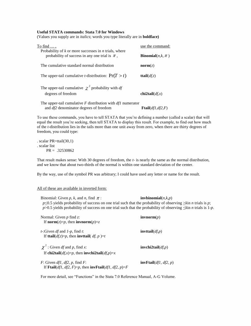
Useful STATA commands: Stata 7.0 for Windows
(Values you supply are in italics; words you type literally are in boldface)
To find … , use the command:
Probability of k or more successes in n trials, where
probability of success in any one trial is , Binomial(n,k, )
The cumulative standard normal distribution norm(z)
The upper-tail cumulative t-distribution: )Pr( tT ttail(df,t)
The upper-tail cumulative 2
probability with df
degrees of freedom chi2tail(df,x)
The upper-tail cumulative F distribution with df1 numerator
and df2 denominator degrees of freedom Ftail(df1,df2,F)
To use these commands, you have to tell STATA that you’re defining a number (called a scalar) that will
equal the result you’re seeking, then tell STATA to display this result. For example, to find out how much
of the t-distribution lies in the tails more than one unit away from zero, when there are thirty degrees of
freedom, you could type:
. scalar PR=ttail(30,1)
. scalar list
PR = .32530862
That result makes sense: With 30 degrees of freedom, the t- is nearly the same as the normal distribution,
and we know that about two-thirds of the normal is within one standard deviation of the center.
By the way, use of the symbol PR was arbitrary; I could have used any letter or name for the result.
All of these are available in inverted form:
Binomial: Given p, k, and n, find : invbinomial(n,k,p)
p<0.5 yields probability of success on one trial such that the probability of observing >kin n trials is p;
p>0.5 yields probability of success on one trial such that the probability of observing <kin n trials is 1-p.
Normal: Given p find z: invnorm(p)
If norm(z)=p, then invnorm(p)=z
t-:Given df and 1-p, find t: invttail(df,p)
If ttail(df,t)=p, then invttail( df, p )=t
2
: Given df and p, find x: invchi2tail(df,p)
If chi2tail(df,x)=p, then invchi2tail(df,p)=x
F: Given df1, df2, p, find F: invFtail(df1, df2, p)
If Ftail(df1, df2, F)=p, then invFtail(df1, df2, p)=F
For more detail, see ―Functions‖ in the Stata 7.0 Reference Manual, A-G Volume.
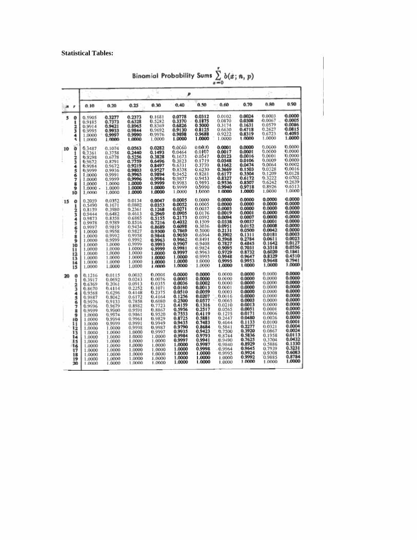
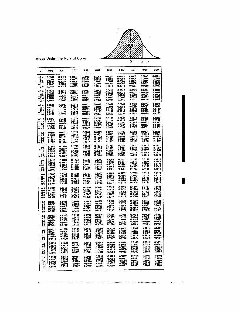
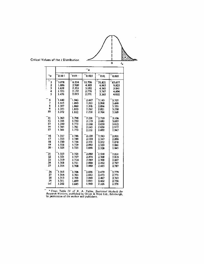
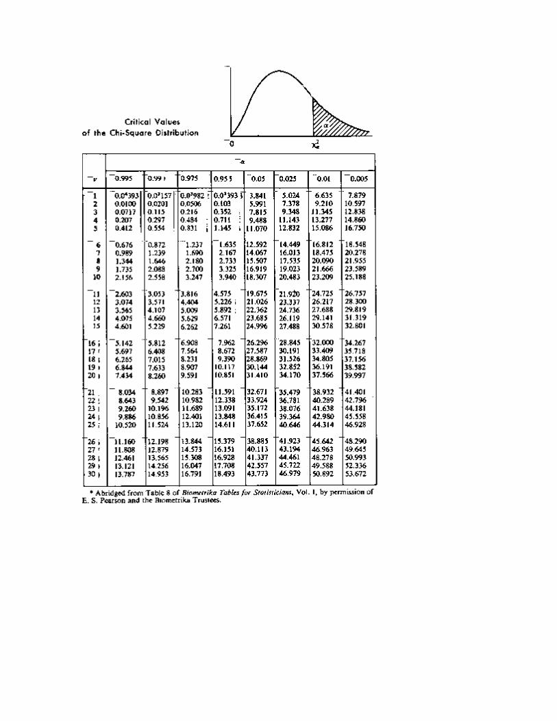
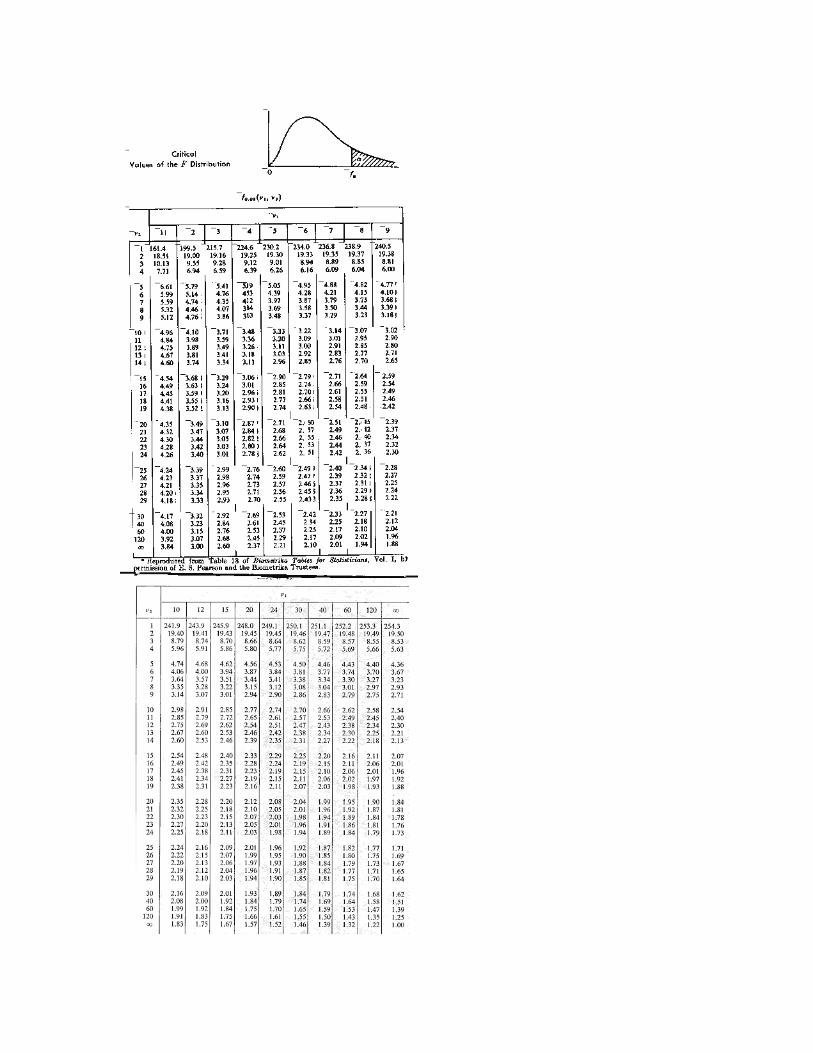
Statistical Tables: