46

CHAPTER 3

ARTIFICIAL NEURAL NETWORKS AND

LEARNING ALGORITHM

3.1 ARTIFICIAL NEURAL NETWORKS

3.1.1 Introduction

The notion of computing takes many forms. Historically, the term

‘computing’ has been dominated by the concept of ‘programmed computing’

than neural computing. In programmed computing, algorithms are designed

and subsequently implemented using the currently dominant architecture,

whereas in neural computing, learning replaces a priori program development.

The neural computing offers a potential solution to many currently unsolved

problems in conventional computing. Artificial neural networks provide new

tools and new foundations for solving practical problems in prediction,

decision and control, signal separation, state estimation, pattern recognition,

data mining, etc. Traditional statistics tries to collect a huge library of

different methods for different tasks, but the brain is a living proof that one

system can do it all, if there is data. It proves that a system can manage

millions of variables without being confused. Nowadays, engineers and

scientists are trying to develop intelligent machines. Artificial Neural Systems

(ANS) are examples of such machines that have greater potential to further

improve the quality of human life.

Artificial neural networks are collections of mathematical models that

emulate some of the observed properties of biological nervous systems and

47

draw on the analogies of adaptive biological learning. They are capable of

developing their behavior through learning. They learn through experiences

like human brain. They are dynamical systems in the learning/training phase

of their operation and convergence is an essential feature. There are different

types of ANNs. Some of the popular models include the BPN which is

generally trained with the Generalized Delta Rule (GDR), Learning Vector

Quantization (LVQ), Radial Basis Function (RBF), Hopfield, Adaptive

Resonance Theory (ART) and Kohonen’s Self-Organizing Feature Map

(SOM) networks. Some ANNs are classified as feedforward while others are

recurrent (i.e., implement feedback) depending on how data is processed

through the network.

The synaptic weight update of ANNs can be carried out by

supervised methods, or by unsupervised methods, or by fixed weight

association network methods. In the case of the supervised methods, inputs

and outputs are used, whereas, in the unsupervised methods, only the inputs

are used. In the fixed weight association network methods, inputs and outputs

are used along with pre-computed and pre-stored weights. Artificial Neural

Networks are used where

• a conventional process is not suitable.

• the conventional method cannot be easily delivered.

• the conventional method cannot fully capture the complexity

in the data and the stochastic behavior is important.

• an explanation of the network’s decision is not required.

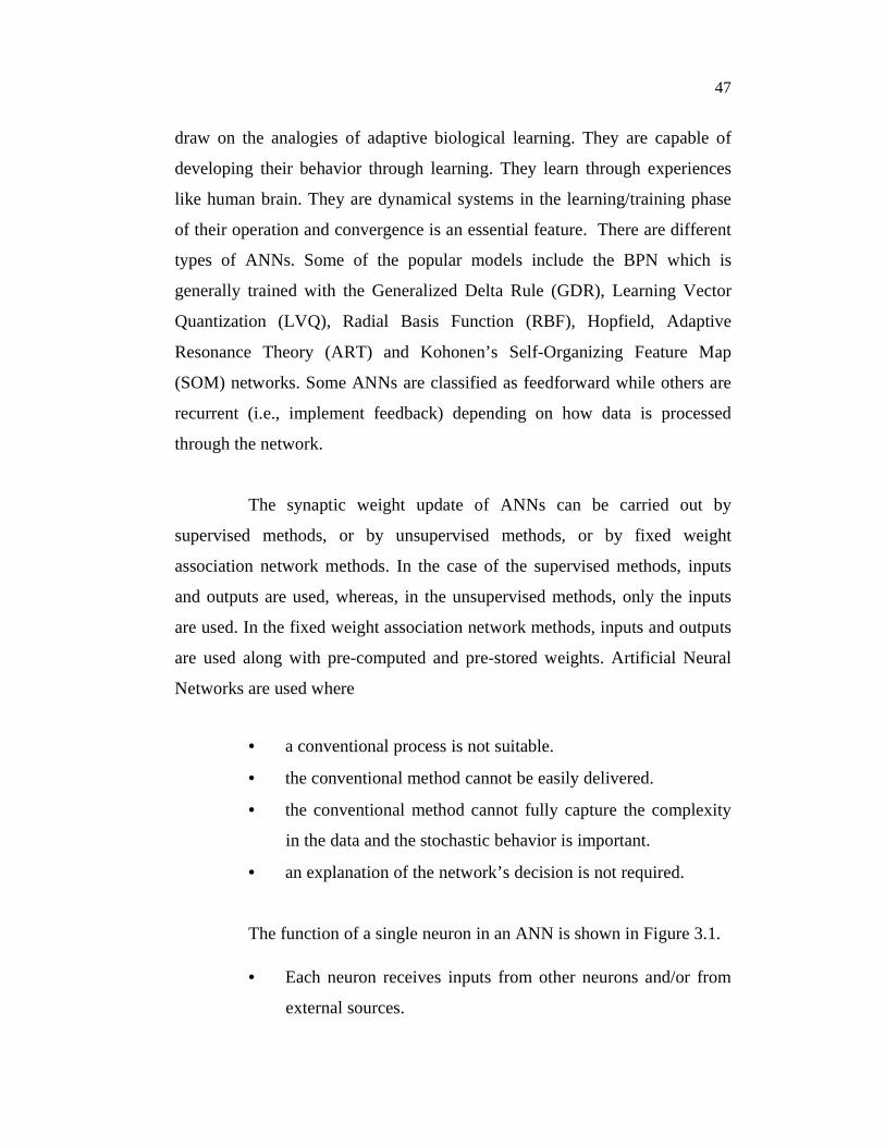
The function of a single neuron in an ANN is shown in Figure 3.1.

• Each neuron receives inputs from other neurons and/or from

external sources.

48

• Like a real neuron, the processing element has many inputs

but has only a single output, which is connected to many other

processing elements in the network.

• Each processing element is numbered. It applies

linear/nonlinear function on its net input to compute the

output.

Figure 3.1 Function of a single neuron

In the above Figure, the input pattern is represented by

[ ]T

1 2 nX x ,x ,......., x= (3.1)

Each artificial neuron’s input has an associated weight which

indicates the fraction (or amount) of the transfer of one neuron’s output to

another neuron’s input. The inputs for an artificial neuron are from external

sources or from other neurons. The notation ‘wij ’ is used to represent the

weight on the interconnection link from neuron ‘j’ to neuron ‘i’. The weight

vector ‘W’ is represented as

[ ]T

1 2 nW w ,w ,.......,w= (3.2)

49

The net input value of a single neuron is determined by the

weighted sum of inputs as given by

i i1 1 i2 2 in nnet(i) net w x w x ............ w x= = + + + (3.3)

= n

ik kk 1

w x=∑ (3.4)

where ‘n’ is the number of inputs. A neuron (or unit) fires, if the sum of its

inputs exceeds some threshold value. If it fires, it produces an output, which

has been sent to the next layer neurons.

In vector notation, the net input value is given by

Tinet W X= (3.5)

The output value of a single neuron is obtained as

io(i) f (net )= (3.6)

The objective of neural network design is to determine an optimal

set of weights w*. Therefore, the artificial neurons involve two important

processes.

(i) Determine the net input value by combining the inputs.

(ii) Mapping the net input value into the neuron’s output. This

mapping may be as simple as using the identity function or as

complex as using a nonlinear function.

3.1.2 Backpropagation Neural Network

The area of speech signal separation and recovery of original signals

from a mixed signal is a challenging domain for information and system

processing. Continued attempt of using artificial neural network in speech

50

signal separation is taking place (Cichocki and Unbehauen 1996; Amari and

Cichocki 1998; Meyer et al 2006). They have ensured the separation of

extremely weak or badly scaled stationary signals, as well as a successful

separation even if the mixing matrix is very ill-conditioned.

The Backpropagation (BPN) neural network is a multilayer

supervised neural network which uses steepest descent method to update

weights. Its architecture as given in Figure 3.2 has an input layer with ‘I’

nodes and an output layer with ‘K’ nodes and one hidden layer with ‘J’ nodes.

Each neuron in the hidden layer has its own input weights and the output of a

neuron in a layer goes to all neurons in the next layer.

Figure 3.2 Architecture of backpropagation neural network

The initial weight values are randomly generated by the Matlab function

rand(). The input layer does not process the mixture input. It just distributes

the input samples to all the neurons in the hidden layer. The output of each

hidden layer neuron is obtained by applying the sigmoid function to its net

51

input value. Each hidden neuron output is fed to all the neurons in the output

layer. Each neuron in the output layer, first calculates the net input value and

then it applies nonlinear function on the net input to produce an output value

‘m’.

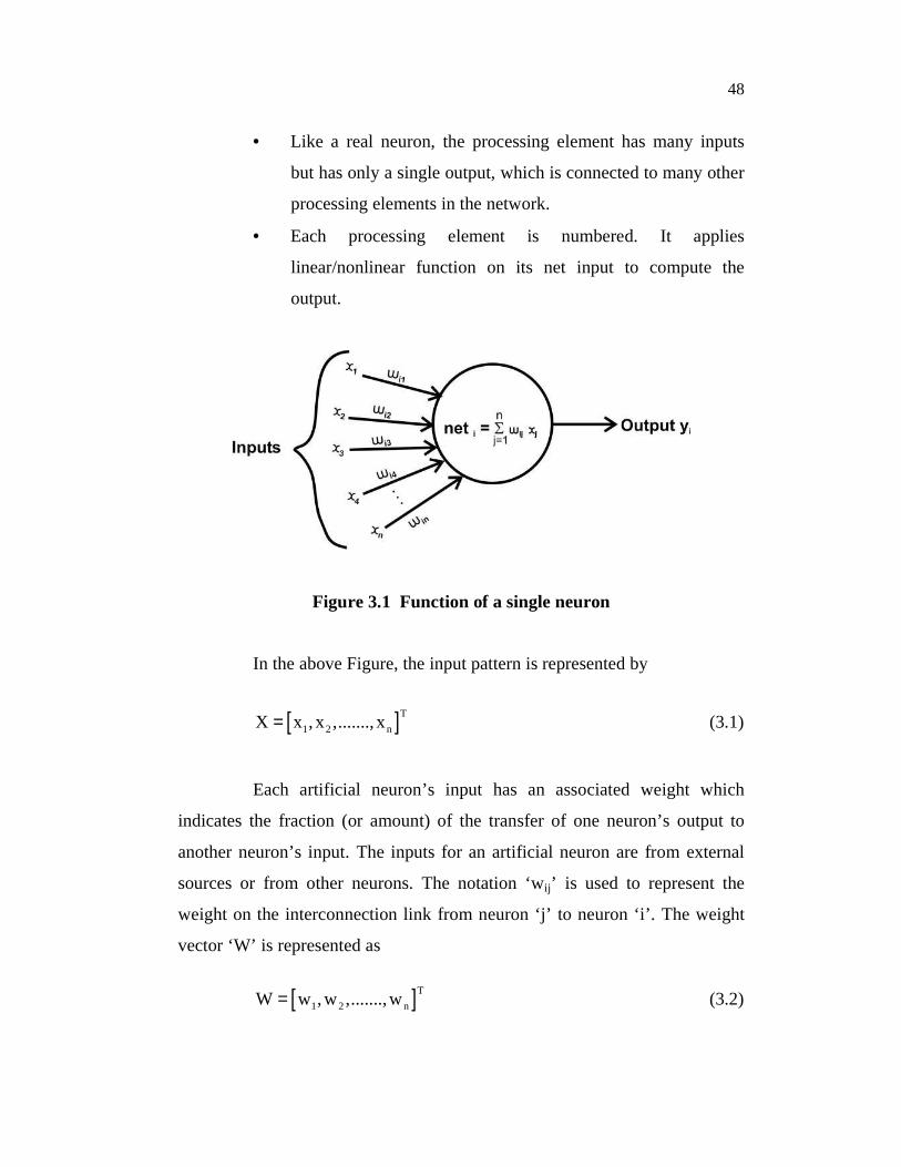
In the earlier stage of this work, an attempt has been made to

extract the individual speech signals from an artificially mixed speech signal

using Backpropagation neural network and its performance is compared with

RBF neural network. To compare their performance, the waveforms of

speeches of only two persons are recorded in a closed environment for two

seconds at the rate of 8KHz. The schematic diagram of speech signal recovery

by BPN neural network is shown in Figure 3.3.

Training

`

Testing

Figure 3.3 Schematic diagram of speech signal recovery

4000 samples of each speech signal shown in Figure 3.4 are mixed and are

used for training the BPN network.

52

(a) Speech signals of two persons

(b) Mixed speech signal

Figure 3.4 Two speech signals and mixed signal

(a) Recovery of speech 1 (b) Recovery of speech 2

Figure 3.5 Recovery of speech signals by BPN neural network

(a) Recovery of speech 1 (b) Recovery of speech 2

Figure 3.6 Recovery of speech signals by RBF neural network

53

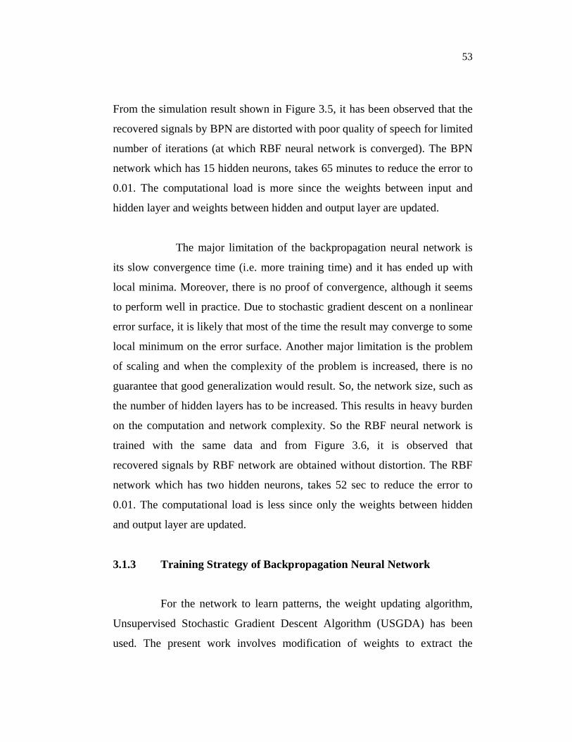
From the simulation result shown in Figure 3.5, it has been observed that the

recovered signals by BPN are distorted with poor quality of speech for limited

number of iterations (at which RBF neural network is converged). The BPN

network which has 15 hidden neurons, takes 65 minutes to reduce the error to

0.01. The computational load is more since the weights between input and

hidden layer and weights between hidden and output layer are updated.

The major limitation of the backpropagation neural network is

its slow convergence time (i.e. more training time) and it has ended up with

local minima. Moreover, there is no proof of convergence, although it seems

to perform well in practice. Due to stochastic gradient descent on a nonlinear

error surface, it is likely that most of the time the result may converge to some

local minimum on the error surface. Another major limitation is the problem

of scaling and when the complexity of the problem is increased, there is no

guarantee that good generalization would result. So, the network size, such as

the number of hidden layers has to be increased. This results in heavy burden

on the computation and network complexity. So the RBF neural network is

trained with the same data and from Figure 3.6, it is observed that

recovered signals by RBF network are obtained without distortion. The RBF

network which has two hidden neurons, takes 52 sec to reduce the error to

0.01. The computational load is less since only the weights between hidden

and output layer are updated.

3.1.3 Training Strategy of Backpropagation Neural Network

For the network to learn patterns, the weight updating algorithm,

Unsupervised Stochastic Gradient Descent Algorithm (USGDA) has been

used. The present work involves modification of weights to extract the

54

independent signals from mixed signals. The function of the network is based

on an unsupervised learning strategy.

The inputs of a pattern are presented and the output of the network

in the output layer is computed and the weights in the output layer and hidden

layer are updated by the weight update equation and compared with the

previous weight value. The total error i.e., the difference between the previous

weight value and the current weight value is determined. The total error for all

patterns presented is calculated and if this total error is greater than zero, the

learning rate parameter is varied by the Equation (4.1) and the weights are

updated by the weight update Equations (3.7) and (3.8). At each iteration, this

process decreases the total error of the network for all the patterns presented.

To minimize the total error to zero, the network is presented with all the

training patterns many times. This procedure is repeated until the error

becomes 0.01.

As given in Figure 3.2, ‘R’ is the weight matrix between input and

hidden layer. ‘Z’ is the weight matrix between the hidden and output layer.

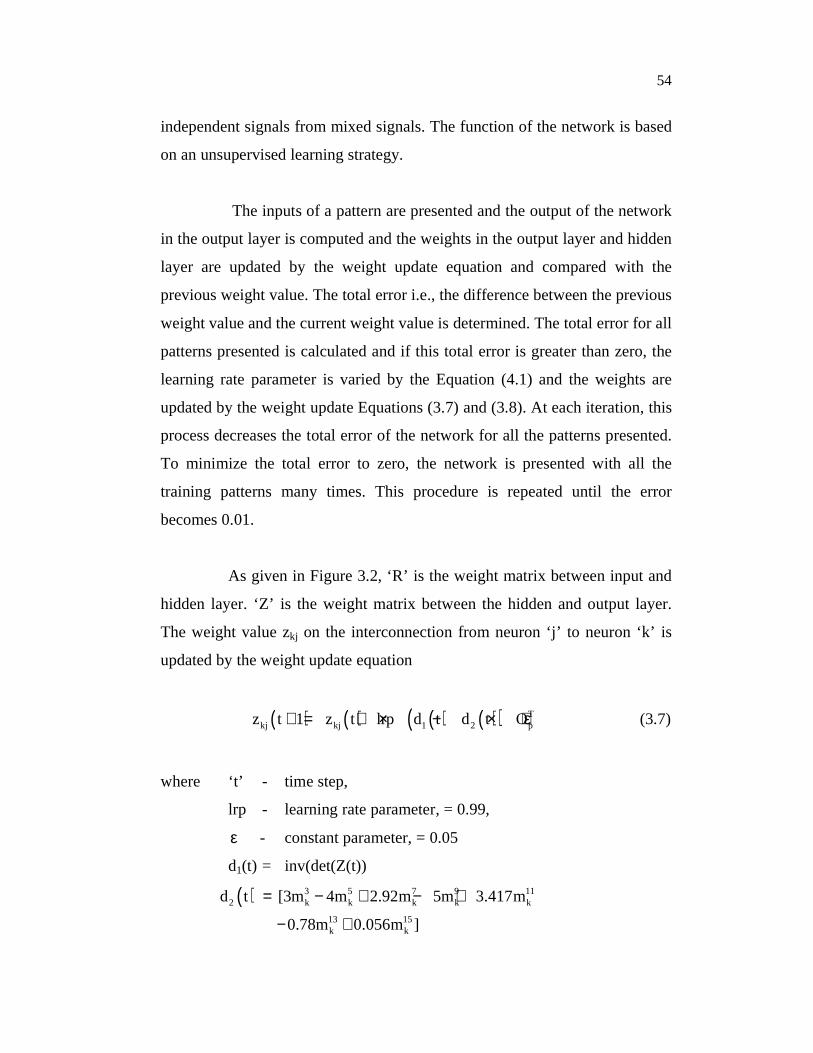
The weight value zkj on the interconnection from neuron ‘j’ to neuron ‘k’ is

updated by the weight update equation

( ) ( ) ( ) ( )( ) Tkj kj 1 2 pz t 1 z t lrp d t d t O+ = + × − × + ε (3.7)

where ‘t’ - time step,

lrp - learning rate parameter, = 0.99,

ε - constant parameter, = 0.05

d1(t) = inv(det(Z(t))

( ) 3 5 7 9 11

2 k k k k k

13 15k k

d t [3m 4m 2.92m 5m 3.417m

0.78m 0.056m ]

= − + − +

− +

55

TpO - Transpose of mixture signal ‘p’

Similarly, all the remaining weights between hidden and output

layer are updated by the Equation (3.7). The weight value rji on the

interconnection from neuron ‘i’ to neuron ‘j’ is updated by the weight update

equation

( ) ( ) ( ) ( )( )( ) ( ) ( ) 1Tji ji 1 2 p kj pjr t 1 z t lrp d t d t O z t 1 exp( net

−+ = + × − × + ε × × + −

(3.8)

Similarly, all the remaining weights between input and hidden layer are

updated by the Equation (3.8).

To implement this algorithm, the speeches of two persons are

recorded in a closed environment for two seconds at the rate of 4 KHz. Like

this, 25 speeches of males and 25 speeches of females are recorded and stored

as .wav files. Fifty combinations (one male and one female; two males; two

females) of different speech waveforms (S1 and S2) are mixed artificially by

multiplying the speech signals with various coefficients as given by

O1 = 0.3×S1+0.7×S2 (3.9)

500 samples of each mixture signal are preprocessed by the

technique, normalization so that the inputs to the nodes of the input layer are

between zero and one. 40 mixture signals are used for training both BPN and

RBF neural networks by the unsupervised stochastic gradient descent

algorithm and 10 mixture signals are used for testing the networks. From

Figure 3.7, it is found that after certain number of iterations (no. of

iterations=2223, at which the RBF network is converged), the BPN network is

able to converge to only some extent. The network is found to convergence

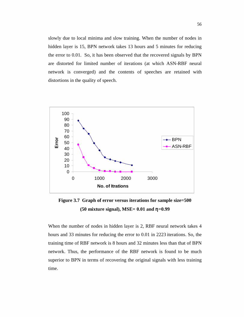
56

slowly due to local minima and slow training. When the number of nodes in

hidden layer is 15, BPN network takes 13 hours and 5 minutes for reducing

the error to 0.01. So, it has been observed that the recovered signals by BPN

are distorted for limited number of iterations (at which ASN-RBF neural

network is converged) and the contents of speeches are retained with

distortions in the quality of speech.

0102030405060708090

100

0 1000 2000 3000

No. of Itrations

Err

or BPN

ASN-RBF

Figure 3.7 Graph of error versus iterations for sample size=500

(50 mixture signal), MSE= 0.01 and ηηηη=0.99

When the number of nodes in hidden layer is 2, RBF neural network takes 4

hours and 33 minutes for reducing the error to 0.01 in 2223 iterations. So, the

training time of RBF network is 8 hours and 32 minutes less than that of BPN

network. Thus, the performance of the RBF network is found to be much

superior to BPN in terms of recovering the original signals with less training

time.

57

3.1.4 Adaptive Self-Normalized Radial Basis Function (ASN-RBF)

Neural Network

In recent years, there has been an increasing interest in using Radial

Basis Function neural network for many problems. Like Backpropagation and

Counter propagation neural networks, it is a feedforward neural network that

is capable of performing nonlinear relationship between the input and output

vector spaces. RBF and BPN are both universal approximators. i.e., when

they are designed with enough hidden layer neurons, they approximate any

continuous function with arbitrary accuracy (Girosi and Poggio 1989;

Hartman et al 1990). This is a property they share with other feedforward

networks having one hidden layer of nonlinear neurons. Hornik et al (1989)

have shown that the nonlinearity need not be sigmoid and it can be any of a

wide range of functions. It is therefore not surprising to find that there always

exists an RBF network capable of accurately mimicking a specified BPN or

vice-versa.

The RBF network is found to be suitable for BSS problem since it has

the following characteristics.

1. It has faster learning capability and it is good at handling

nonlinear data.

2. It finds input to output mapping using local approximators and

they require fewer training samples.

3. It provides smaller interpolation errors, higher reliability and a

more well-developed theoretical analysis than BPN

58

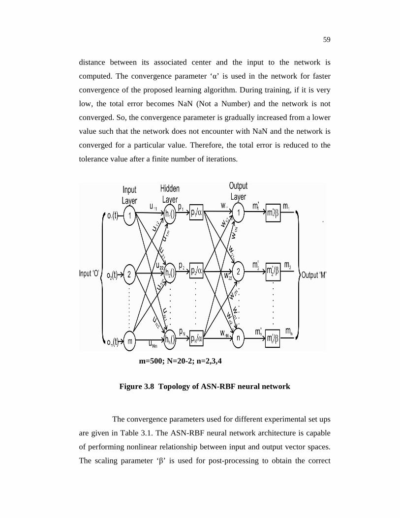
As shown in Figure 3.8, the ASN-RBF neural network consists of three

layers: an input layer with 500 neurons, a single layer of nonlinear processing

neurons and an output layer with 2, 3 or 4 neurons depending on the number

of sources. In Backpropagation neural network, the weights between hidden

layer and output layer and also the weights between hidden and input layer

are updated during training. But, in RBF neural network, only the weights

between hidden and output layer are updated. The RBF network does not end

up with local minima and the outputs of the hidden layer neurons are

calculated by

( ) ( ) ( )k

m mp f o u o,c u o ci i ik k k ik k

k 1 k 1= = ϕ = ϕ −∑ ∑

= =

for i 1,2,...., N= (3.10)

and the outputs of output layer neurons are calculated by

N

ji ii 1

j

w .pm =

= β

∑ where

1β =α

(3.11)

where ip is the output of the hidden neuron ‘i’, ‘α’ is the convergence

parameter used in the network, n 1o R +∈ is an input vector and ( )k .ϕ is a radial

basis function which is given by ( )2 2iexp( D ) 2− λ , where

( ) ( )T2i ji jiD O W O W= − − and ‘λ’ is the spread factor which controls the

width of the radial basis function, ikU is the weight matrix between input and

hidden layer, jiW is the weight matrix between hidden and output layer, ‘N’ is

the number of neurons in the hidden layer and N 1kc R ×∈ are the RBF centers

in the input vector space. For each neuron in the hidden layer, the Euclidean

59

distance between its associated center and the input to the network is

computed. The convergence parameter ‘α’ is used in the network for faster

convergence of the proposed learning algorithm. During training, if it is very

low, the total error becomes NaN (Not a Number) and the network is not

converged. So, the convergence parameter is gradually increased from a lower

value such that the network does not encounter with NaN and the network is

converged for a particular value. Therefore, the total error is reduced to the

tolerance value after a finite number of iterations.

m=500; N=20-2; n=2,3,4

Figure 3.8 Topology of ASN-RBF neural network

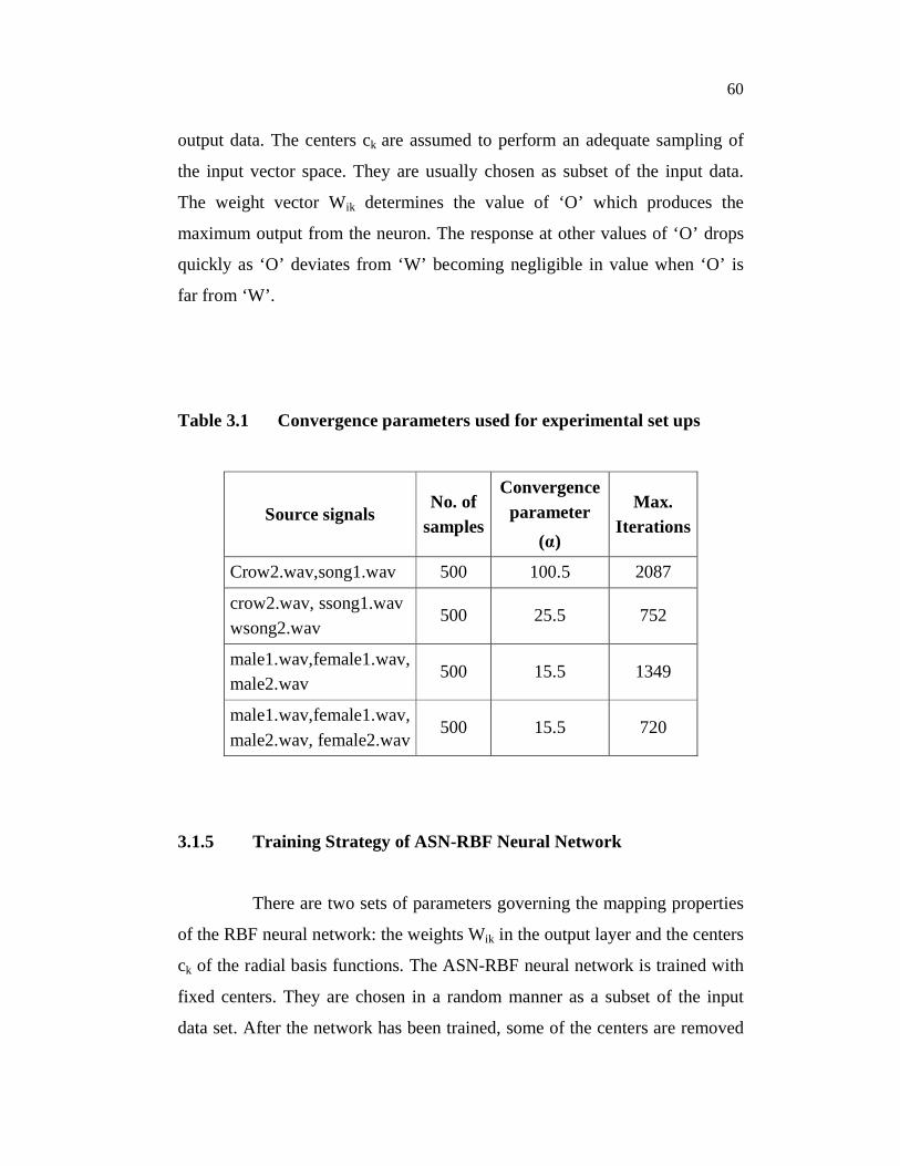
The convergence parameters used for different experimental set ups

are given in Table 3.1. The ASN-RBF neural network architecture is capable

of performing nonlinear relationship between input and output vector spaces.

The scaling parameter ‘β’ is used for post-processing to obtain the correct

60

output data. The centers ck are assumed to perform an adequate sampling of

the input vector space. They are usually chosen as subset of the input data.

The weight vector Wik determines the value of ‘O’ which produces the

maximum output from the neuron. The response at other values of ‘O’ drops

quickly as ‘O’ deviates from ‘W’ becoming negligible in value when ‘O’ is

far from ‘W’.

Table 3.1 Convergence parameters used for experimental set ups

Source signals No. of

samples

Convergence parameter

(α)

Max. Iterations

Crow2.wav,song1.wav 500 100.5 2087

crow2.wav, ssong1.wav wsong2.wav

500 25.5 752

male1.wav,female1.wav, male2.wav

500 15.5 1349

male1.wav,female1.wav, male2.wav, female2.wav

500 15.5 720

3.1.5 Training Strategy of ASN-RBF Neural Network

There are two sets of parameters governing the mapping properties

of the RBF neural network: the weights Wik in the output layer and the centers

ck of the radial basis functions. The ASN-RBF neural network is trained with

fixed centers. They are chosen in a random manner as a subset of the input

data set. After the network has been trained, some of the centers are removed

61

in a systematic manner without significant degradation of the system

performance. The location of the centers of the receptive fields is a critical

issue and there are many alternatives for their determination. In the learning

algorithm, the center and corresponding hidden layer neuron are located at

each input vector in the training set. The diameter of the receptive region,

determined by the value of the spread factor ‘λ’ is set at 0.01, has a profound

effect upon the accuracy of the system. The objective is to cover the input

space with receptive fields as uniformly as possible. If the spacing between

centers is not uniform, it is necessary for each hidden neuron to have its own

value of ‘λ’.

100 inputs (birds voices) are used for this proposed network. Out of

these, 80 inputs are used for training the ASN-RBF neural network and 20

inputs are used for testing the network. Each input corresponds to different

combinations of birds voices downloaded from the website

http://www.nhl.nl/~ribot/english/sounds1.html. Different combinations of the

birds voices are artificially mixed and preprocessed by the technique,

Normalization so that the inputs to the nodes of input layer are between zero

and one. The preprocessed input is fed to the network in the form of 500

samples, corresponding to 500 neurons in the input layer. The number of

source signals is varied from two to four. The ASN-RBF neural network is

also trained and tested for separation of speech signals which are recorded for

about 2 sec in a closed environment at the rate of 8 KHz. The proposed ASN-

RBF neural network and learning algorithm perform well under non-

stationary environments and when the number of source signals is unknown

and dynamically changed.

62

3.2 UNSUPERVISED STOCHASTIC GRADIENT DESCENT

LEARNING ALGORITHM

To separate independent components from the observed signal, an

objective function is required. The objective function is chosen such that it

gives original signals when it is minimized. During training of the ASN-RBF

neural network, one of the free parameters i.e., the interconnection weights

between hidden layer and output layer are adjusted to minimize the objective

function. In signal processing (Taleb and Jutten 1998), when the components

of the output vector become independent, its joint probability density function

factorizes to marginal pdfs, given by

( ) ( )i

k

M M ii 1

f M,W f m ,W=

= ∏ (3.12)

where )W,m(f iM i is the marginal pdf of Mi , mi is the ith component of the

output signal ‘M’ and ‘k’ is the number of source signals. The Equation (3.12)

is a constraint imposed on the learning algorithm. The joint pdf of ‘M’

parameterized by ‘W’ is written as

( )( )

M

f Oof M,W

B= (3.13)

where B is the determinant of the Jacobian matrix ‘B’. It is defined as

1 1 1

1 2 k

2 2 2

1 2 k

k k k

1 2 k

m m m...

o o o

m m m...

o o oB

... ... ... ...

m m m...

o o o

∂ ∂ ∂∂ ∂ ∂∂ ∂ ∂∂ ∂ ∂=

∂ ∂ ∂∂ ∂ ∂

(3.14)

63

Referring to Equation (1.4), each element in Equation (3.14) is

represented interms of ‘w’ as

iij

j

mw

o

∂ =∂

(3.15)

Therefore, Equation (3.14) is written as

11 12 1k

21 22 2k

k1 k2 kk

w w ... w

w w ... wW

... ... ... ...

w w ... w

= (3.16)

Now, Equation (3.13) is written as

( )( )

M

f Oof M,WW

= (3.17)

To extract independent components from the observed signal, the

difference between the joint pdf and the product of marginal pdfs is

determined. When the components become independent, the difference

becomes zero (i.e. the joint pdf becomes equal to the product of marginal pdfs

of the separated signals). It is expressed as

( ) ( )i

k

M M ii 1

f M,W f m ,W 0=

− =∏ (3.18)

Since the logarithm provides computational simplicity, it is taken

on both sides of Equation (3.18) and it becomes,

( ) ( )( )i

k

M M ii 1

log(f M,W) log f m ,W=

=∑ (3.19)

64

Substituting the value of ( )Mf m,W from Equation (3.17) in

Equation (3.19),

( ) ( )( )

i

ko

M ii 1

f Olog log f m ,W

W =

=

∑ (3.20)

Because the pdf of the input vector is independent of the parameter

vector ‘W’, the objective function for optimization becomes

( ) ( )i

k

M ii 1

(W) log W log f (m ,W)=

Φ = − −∑ (3.21)

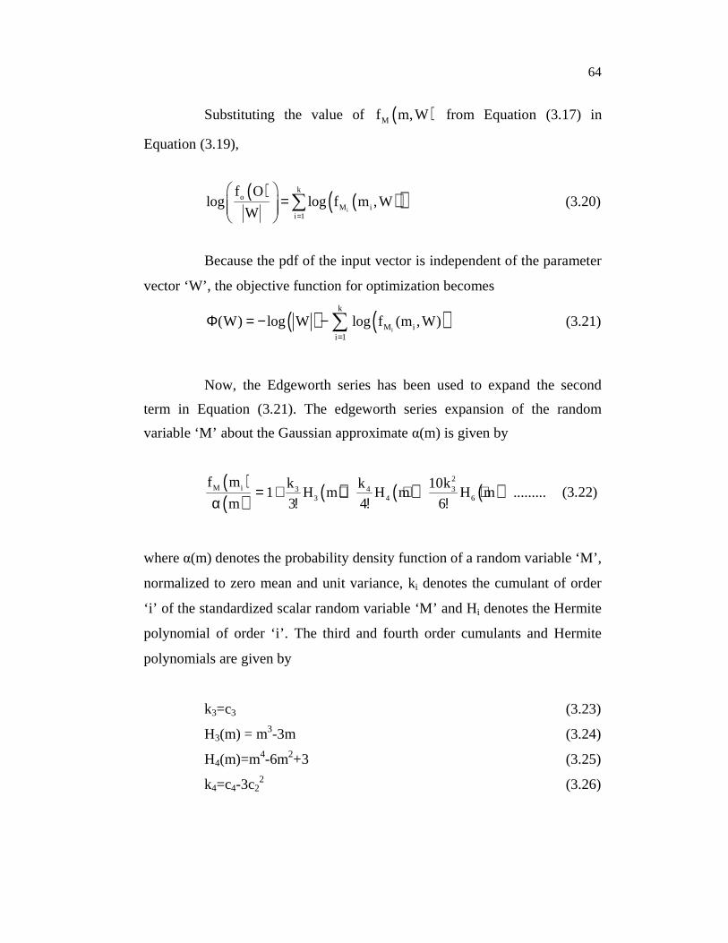
Now, the Edgeworth series has been used to expand the second

term in Equation (3.21). The edgeworth series expansion of the random

variable ‘M’ about the Gaussian approximate α(m) is given by

( )( ) ( ) ( ) ( )

2M i 3 34

3 4 6

f m k 10kk1 H m H m H m .........

m 3 4 6= + + + +

α ! ! ! (3.22)

where α(m) denotes the probability density function of a random variable ‘M’,

normalized to zero mean and unit variance, ki denotes the cumulant of order

‘i’ of the standardized scalar random variable ‘M’ and Hi denotes the Hermite

polynomial of order ‘i’. The third and fourth order cumulants and Hermite

polynomials are given by

k3=c3 (3.23)

H3(m) = m3-3m (3.24)

H4(m)=m4-6m2+3 (3.25)

k4=c4-3c22 (3.26)

65

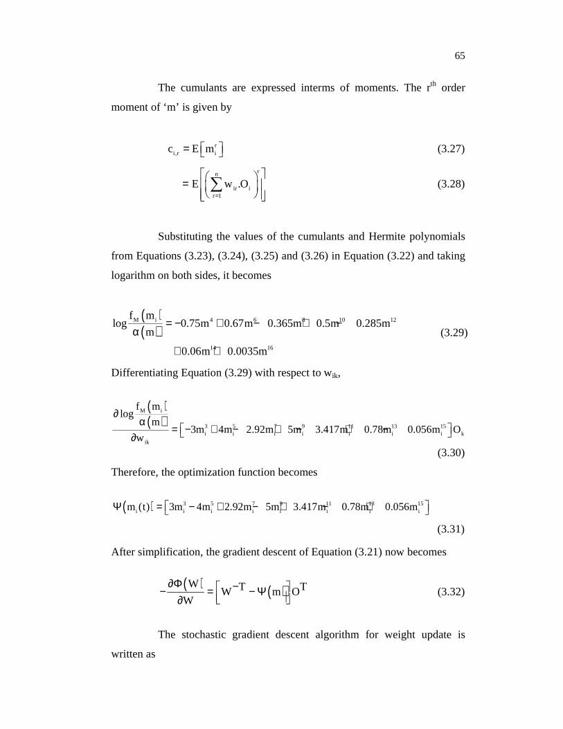
The cumulants are expressed interms of moments. The rth order

moment of ‘m’ is given by

ri,r ic E m = (3.27)

rn

ir ir 1

E w .O=

= ∑ (3.28)

Substituting the values of the cumulants and Hermite polynomials

from Equations (3.23), (3.24), (3.25) and (3.26) in Equation (3.22) and taking

logarithm on both sides, it becomes

( )( )

4 6 8 10 12M i

14 16

f mlog 0.75m 0.67m 0.365m 0.5m 0.285m

m

0.06m 0.0035m

= − + − + −α

+ +

(3.29)

Differentiating Equation (3.29) with respect to wik,

( )( )

M i

3 5 7 9 11 13 15i i i i i i i k

ik

f mlog

m3m 4m 2.92m 5m 3.417m 0.78m 0.056m O

w

∂α

= − + − + − + − ∂ (3.30)

Therefore, the optimization function becomes

( ) 3 5 7 9 11 13 15i i i i i i i im (t) 3m 4m 2.92m 5m 3.417m 0.78m 0.056m Ψ = − + − + − +

(3.31)

After simplification, the gradient descent of Equation (3.21) now becomes

( ) ( )W T TW m OW

∂Φ − − = − Ψ ∂

(3.32)

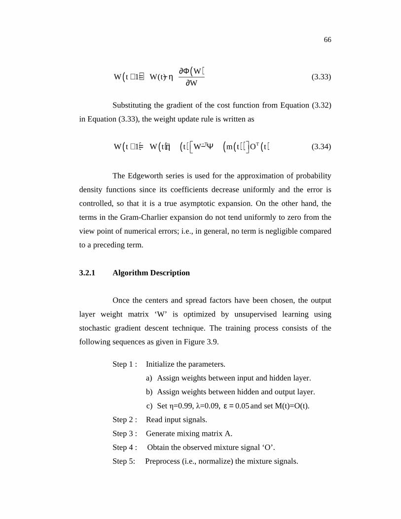
The stochastic gradient descent algorithm for weight update is

written as

66

( ) ( )WW t 1 W(t)

W

∂Φ+ = − η

∂ (3.33)

Substituting the gradient of the cost function from Equation (3.32)

in Equation (3.33), the weight update rule is written as

( ) ( ) ( ) ( )( ) ( )T TW t 1 W t t W m t O t− + = + η − Ψ (3.34)

The Edgeworth series is used for the approximation of probability

density functions since its coefficients decrease uniformly and the error is

controlled, so that it is a true asymptotic expansion. On the other hand, the

terms in the Gram-Charlier expansion do not tend uniformly to zero from the

view point of numerical errors; i.e., in general, no term is negligible compared

to a preceding term.

3.2.1 Algorithm Description

Once the centers and spread factors have been chosen, the output

layer weight matrix ‘W’ is optimized by unsupervised learning using

stochastic gradient descent technique. The training process consists of the

following sequences as given in Figure 3.9.

Step 1 : Initialize the parameters.

a) Assign weights between input and hidden layer.

b) Assign weights between hidden and output layer.

c) Set η=0.99, λ=0.09, 0.05ε = and set M(t)=O(t).

Step 2 : Read input signals.

Step 3 : Generate mixing matrix A.

Step 4 : Obtain the observed mixture signal ‘O’.

Step 5: Preprocess (i.e., normalize) the mixture signals.

67

Step 6 : Recover source signals.

(i) Apply the observed signal to the input layer neurons.

% Forward operation

% For each pattern in the training set

a) Find the Hidden layer output.

b) Find inputs to nodes in the output layer.

c) Compute the actual output of output layer

neurons.

d) Determine delta ∆W.

e) Update the weights between hidden and output

layer.

f) If the difference between previous weight value

and current weight value is not equal to zero,

then

go to step 5

else

stop training

Step 7: Postprocess (i.e., Denormalization) the output data.

Step 8: Store and display the separated signals.

Thus, the development of this algorithm involves

maximization of the statistical independence between the output vectors

‘M’. It is equivalent to minimizing the divergence between the two

distributions:

(i) Joint probability density function fM(m,W) parameterized

by W.

68

(ii) Product of marginal density function of Mi,

( )n

M iii 1

f m ,W=

∏ .

Figure 3.9 Block diagram of source signal recovery

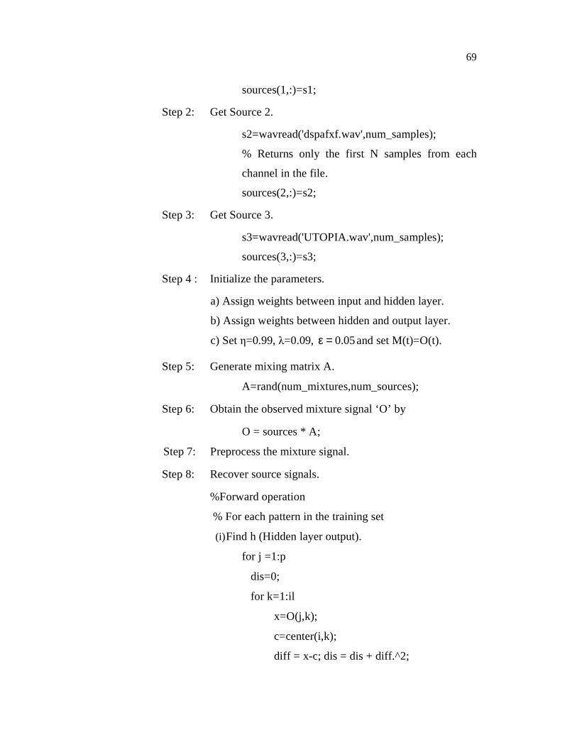
3.2.2 Implementation of USGDA

Step 1: Get Source 1.

[s1,srate,no_bits]=wavread('nukeanthem');

% Returns the sample rate in Hertz and the

number of bits per sample (NBITS) used to

encode the data in the file.

s1=wavread('nukeanthem.wav',num_samples);

69

sources(1,:)=s1;

Step 2: Get Source 2.

s2=wavread('dspafxf.wav',num_samples);

% Returns only the first N samples from each

channel in the file.

sources(2,:)=s2;

Step 3: Get Source 3.

s3=wavread('UTOPIA.wav',num_samples);

sources(3,:)=s3;

Step 4 : Initialize the parameters.

a) Assign weights between input and hidden layer.

b) Assign weights between hidden and output layer.

c) Set η=0.99, λ=0.09, 0.05ε = and set M(t)=O(t).

Step 5: Generate mixing matrix A.

A=rand(num_mixtures,num_sources);

Step 6: Obtain the observed mixture signal ‘O’ by

O = sources * A;

Step 7: Preprocess the mixture signal.

Step 8: Recover source signals.

%Forward operation

% For each pattern in the training set

(i) Find h (Hidden layer output).

for j =1:p

dis=0;

for k=1:il

x=O(j,k);

c=center(i,k);

diff = x-c; dis = dis + diff.^2;

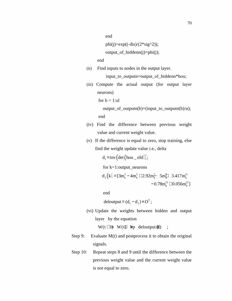
70

end

phi(j)=exp((-dis)/(2*sig^2));

output_of_hiddenn(j)=phi(j);

end

(ii) Find inputs to nodes in the output layer.

input_to_outputn=output_of_hiddenn*hou;

(iii) Compute the actual output (for output layer

neurons)

for b = 1:ol

output_of_outputn(b)=(input_to_outputn(b)/α);

end

(iv) Find the difference between previous weight

value and current weight value.

(v) If the difference is equal to zero, stop training, else

find the weight update value i.e., delta

( )( )1d inv det hou _ old ;=

for k=1:output_neurons

( ) 3 5 7 9 11

2 k k k k k

13 15k k

d k [3m 4m 2.92m 5m 3.417m

0.78m 0.056m ]

= − + − +

− +

end

T1 2deloutput (d d ) O= − × ;

(vi) Update the weights between hidden and output

layer by the equation

W(t 1) W(t) lrp deloutput (t) ;+ = + × + ε

Step 9: Evaluate M(t) and postprocess it to obtain the original

signals.

Step 10: Repeat steps 8 and 9 until the difference between the

previous weight value and the current weight value

is not equal to zero.

71

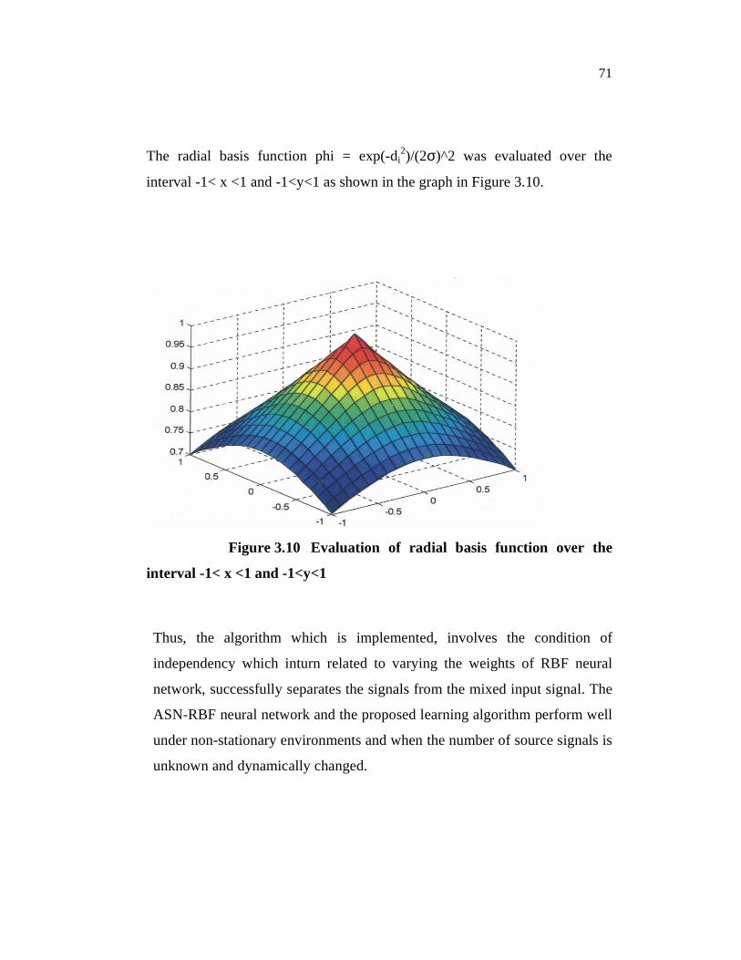
The radial basis function phi = exp(-di2)/(2σ)^2 was evaluated over the

interval -1< x <1 and -1<y<1 as shown in the graph in Figure 3.10.

Figure 3.10 Evaluation of radial basis function over the

interval -1< x <1 and -1<y<1

Thus, the algorithm which is implemented, involves the condition of

independency which inturn related to varying the weights of RBF neural

network, successfully separates the signals from the mixed input signal. The

ASN-RBF neural network and the proposed learning algorithm perform well

under non-stationary environments and when the number of source signals is

unknown and dynamically changed.