chapter 3: answers to questions and...

Chapter 03 - Quantitative Demand Analysis

Chapter 3: Answers to Questions and Problems

1.a. When P = $12, R = ($12)(1) = $12. When P = $10, R = ($10)(2) = $20. Thus, the

price decrease results in an $8 increase in total revenue, so demand is elastic over this range of prices.

b. When P = $4, R = ($4)(5) = $20. When P = $2, R = ($2)(6) = $12. Thus, the price decrease results in an $8 decrease total revenue, so demand is inelastic over this range of prices.

c. Recall that total revenue is maximized at the point where demand is unitary elastic. We also know that marginal revenue is zero at this point. For a linear demand curve, marginal revenue lies halfway between the demand curve and the vertical axis. In this case, marginal revenue is a line starting at a price of $14 and intersecting the quantity axis at a value of Q = 3.5. Thus, marginal revenue is 0 at 3.5 units, which corresponds to a price of $7 as shown below.

$0

$2

$4

$6

$8

$10

$12

$14

0 1 2 3 4 5 6 Quantity

Price

Demand

MR

Figure 3-1

2. a. At the given prices, quantity demanded is 750 units: Q xd=1,200−3 (140 )−0.1 (300 )=750. Substituting the relevant information into the

elasticity formula gives: EQ x , Px=−3PxQx

=−3 140750

=−0.56. Since this is less than

one in absolute value, demand is inelastic at this price. If the firm charged a lower price, total

3-1© 2014 by McGraw-Hill Education. This is proprietary material solely for authorized instructor use. Not authorized for sale or distribution

in any manner. This document may not be copied, scanned, duplicated, forwarded, distributed, or posted on a website, in whole or part.


revenue would decrease.b. At the given prices, quantity demanded is 450 units: Q xd=1,200−3 (240 )−0.1 (300 )=450. Substituting the relevant information into

the elasticity formula gives: EQ x , Px=−3P xQx

=−3 240750

=−1.6. Since this is greater

than one in absolute value, demand is elastic at this price. If the firm increased its price, total revenue would decrease.

c. At the given prices, quantity demanded is 750 units, as shown in part a. Substituting the relevant information into the elasticity formula gives:

EQ x , Pz=−0.1P zQ x

=−0.1 300750

=−0.04 . Since this number is negative, goods X and

Z are complements.

3.a. The own price elasticity of demand is simply the coefficient of ln Px, which is

– 1.5. Since this number is more than one in absolute value, demand is elastic.b. The cross-price elasticity of demand is simply the coefficient of ln Py, which is 2.

Since this number is positive, goods X and Y are substitutes.c. The income elasticity of demand is simply the coefficient of ln M, which is -0.5.

Since this number is negative, good X is an inferior good.d. The advertising elasticity of demand is simply the coefficient of ln A, which is 1.

4.

a. Use the own price elasticity of demand formula to write % ΔQxd

−5=−3. Solving,

we see that the quantity demanded of good X will increase by 15 percent if the price of good X decreases by 5 percent.

b. Use the cross-price elasticity of demand formula to write % ΔQxd

8=−4 . Solving,

we see that the demand for X will decrease by 32 percent if the price of good Y increases by 8 percent.

c. Use the formula for the advertising elasticity of demand to write % ΔQxd

−4=2.

Solving, we see that the demand for good X will decrease by 8 percent if advertising decreases by 4 percent.

d. Use the income elasticity of demand formula to write % ΔQxd

4=1. Solving, we see

that the demand of good X will increase by 4 percent if income increases by 4 percent.

5. Using the cross price elasticity formula,20

% ΔPy=4. Solving, we see that the price of

good Y would have to increase by 5 percent in order to increase the consumption of good X by 20 percent.




6. Using the change in revenue formula for two products, ΔR=[$ 40,000 (1−1.5 )+$90,000 (−1.8 ) ] (0.02 )=−$3,640. Thus, a 2 percent increase in the price of good X would cause revenues from both goods to decrease by $3,640.

7. Table 3-1 contains the answers to the regression output.

SUMMARY OUTPUT

Regression Statistics

Multiple R 0.38R Square 0.14Adjusted R Square 0.13Standard Error 20.77Observations 150

Analysis of Variance

Degrees of Freedom

Sum of Squares Mean Square F Significance F

Regression 2 10,398.87 5199.43 12.05 0.00Residual 147 63,408.62 431.35Total 149 73,807.49

CoefficientsStandard

Error t Stat P-value Lower 95% Upper 95%Intercept 58.87 15.33 3.84 0.00 28.59 89.15Price of X -1.64 0.85 -1.93 0.06 -3.31 0.04Income (‘000s) 1.11 0.24 4.64 0.00 0.63 1.56

Table 3-1

a. Q xd=58.87−1.64Px+1.11M .

b. Only the coefficients for the Intercept and Income are statistically significant at the 5 percent level or better.

c. The R-square is quite low, indicating that the model explains only 14 percent of the total variation in demand for X. The adjusted R-square is only marginally lower (13 percent), suggesting that the R-square is not the result of an excessive number of estimated coefficients relative to the sample size. The F-statistic,




however, suggests that the overall regression is statistically significant at better than the 5 percent level.

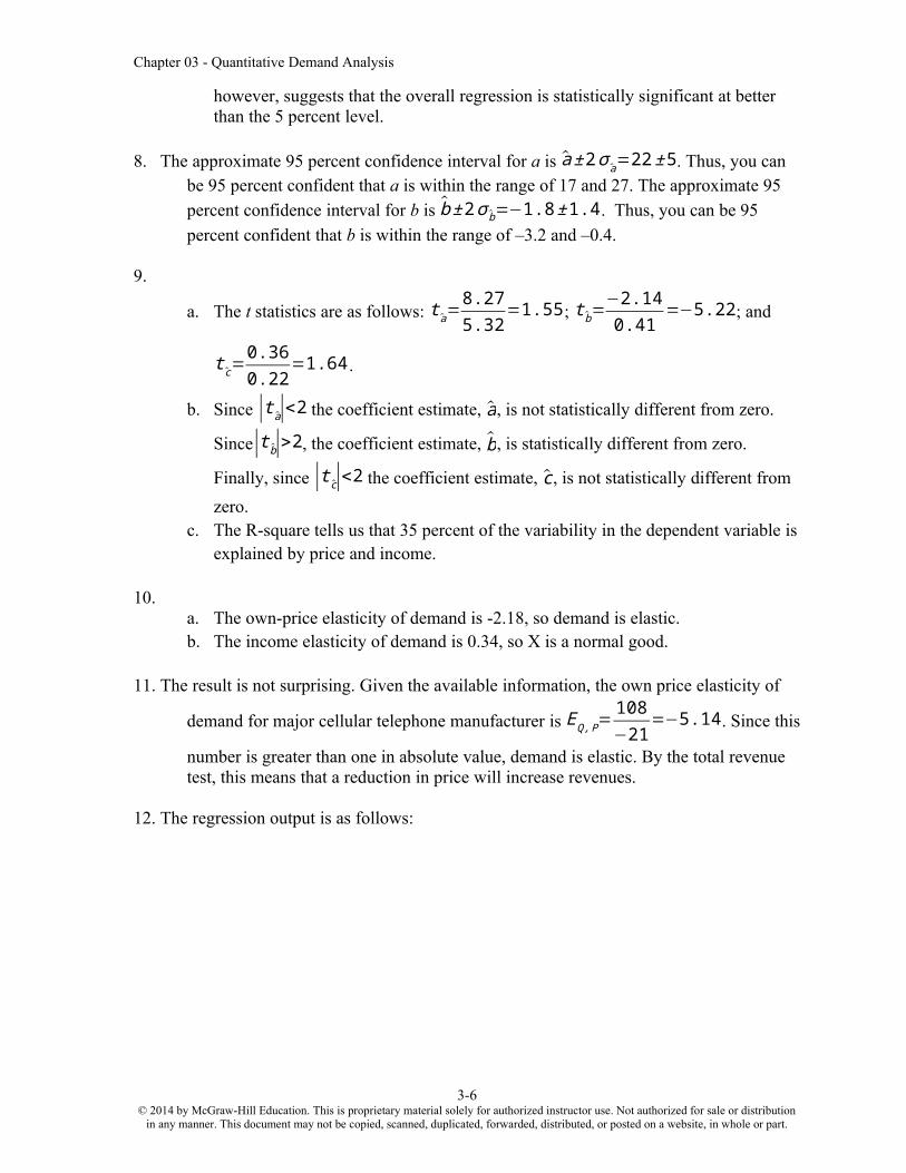
8. The approximate 95 percent confidence interval for a is a ±2σ a=22±5. Thus, you can be 95 percent confident that a is within the range of 17 and 27. The approximate 95 percent confidence interval for b is b ±2σ b=−1.8±1.4. Thus, you can be 95 percent confident that b is within the range of –3.2 and –0.4.

9.

a. The t statistics are as follows: t a=8.275.32

=1.55; t b=−2.140.41

=−5.22; and

t c=0.360.22

=1.64.

b. Since |t a|<2 the coefficient estimate, a, is not statistically different from zero. Since|t b|>2, the coefficient estimate, b, is statistically different from zero. Finally,

since |t c|<2 the coefficient estimate, c, is not statistically different from zero.c. The R-square tells us that 35 percent of the variability in the dependent variable is

explained by price and income.

10.a. The own-price elasticity of demand is -2.18, so demand is elastic.b. The income elasticity of demand is 0.34, so X is a normal good.

11. The result is not surprising. Given the available information, the own price elasticity of

demand for major cellular telephone manufacturer is EQ ,P=108−21

=−5.14. Since this

number is greater than one in absolute value, demand is elastic. By the total revenue test, this means that a reduction in price will increase revenues.

12. The regression output is as follows:




SUMMARY OUTPUT

Regression StatisticsMultiple R 0.97R Square 0.94Adjusted R Square 0.94Standard Error 0.00Observations 49

ANOVAdf SS MS F Significance F

Regression 2 0.00702 0.004 370.38 0.0000Residual 46 0.00044 0.000Total 48 0.00745

Coefficients Standard Error t Stat P-value Lower 95% Upper 95%Intercept 1.29 0.41 3.12 0.00 0.46 2.12LN Price -0.07 0.00 -26.62 0.00 -0.08 -0.07LN Income -0.03 0.09 -0.33 0.74 -0.22 0.16

Table 3-2

Thus, the demand for your batteries is given by lnQ = 1.29 – 0.07lnP – 0.03lnM. Since this is a log-linear demand equation, the best estimate of the income elasticity of demand for your product is -.03: Your batteries are an inferior good. However, note the estimated income elasticity is very close to zero (implying that a 3 percent reduction in global incomes would increase the demand for your product by less than one tenth of one percent). More importantly, the estimated income elasticity is not statistically different from zero (the 95 percent confidence interval ranges from a low of -.22 to a high of .16, with a t-statistic that is well below 2 in absolute value). On balance, this means that a 3 percent decline in global incomes is unlikely to impact the sales of your product. Note that the R-square is reasonably high, suggesting the model explains 94 percent of the total variation in the demand for this product. Likewise, the F-test indicates that the regression fit is highly significant.

13. Based on this information, the own price elasticity of demand for Big G cereal is

EQ ,P=−54

=−1.25. Thus, demand for Big G cereal is elastic (since this number is

greater than one in absolute value). Since Lucky Charms is one particular brand of cereal for which even more substitutes exist, you would expect the demand for Lucky Charms to be even more elastic than the demand for Big G cereal. Thus, since the demand for Lucky Charms is elastic, one would predict that the increase in price of Lucky Charms resulted in a reduction in revenues on sales of Lucky Charms.

14. Use the income elasticity formula to write % ΔQd

6=2.6. Solving, we see that coffee

purchases are expected to increase by 15.6 percent.

15. To maximize revenue, Toyota should charge the price that makes demand unit elastic. Using the own price elasticity of demand formula,




EQ ,P=(−1.5 )( P150,000−1.5 P )=−1. Solving this equation for P implies that the

revenue maximizing price is P = $50,000.

16. Using the change in revenue formula for two products, ∆ R=[$ 400 (1−2 )+$600 (−0.3 ) ]∗(−0.04 )=$ 23.2 million, so revenues will increase by $23.2 million.

17. The estimated demand function for residential heating fuel is QRHFd =136.96−91.69 PRHF+43.88PNG−11.92PE−0.05M , where PRHF is the price of

residential heating fuel, PNG is the price of natural gas, PE is the price of electricity, and M is income. However, notice that coefficients of income and the price of electricity are not statistically different from zero. Among other things, this means that the proposal to increase the price of electricity by $4 is unlikely to have a statistically significant impact on the demand for residential heating fuel. Since the

coefficient of PRHF is -91.69, a $1 increase in PRHF would lead to a 91.69 unit reduction in the consumption of residential heating fuel. Since the coefficient of PNG is 43.88, a $3 reduction in PNG would lead to a 3*43.88 = 131.64 unit reduction in the consumption of residential heating fuel. Thus, the proposal to reduce the price of natural gas by $3 would lead to the greatest expected reduction in the consumption of residential heating fuel.




18. The regression output is as follows:

SUMMARY OUTPUT




Coefficients Standard Error t Stat P-value Lower 95% Upper 95%Intercept 4.29 0.12 37.17 0.00 4.06 4.53ln (Price) -1.38 0.06 -24.48 0.00 -1.50 -1.27

Table 3-3

Thus, the least squares regression line is . The own price elasticity of demand for broilers is –1.38. From the t-statistic, this is statistically different from zero (the t-statistic is well over 2 in absolute value). The R-square is relatively high, suggesting that the model explains 94 percent of the total variation in the demand for chicken. Given that your current revenues are $750,000 and the elasticity of demand is –1.38, we may use the following formula to determine how much you must change price to increase revenues by $50,000:

ΔR=[Px⋅Q x (1+EQ x ,P x) ]×ΔPxP x

$50 ,000=[ $750 ,000 (1−1.38 ) ]ΔP xPx

Solving yields

ΔPxPx

= $50 ,000−$285 ,000

=−0 .175. That is, to increase revenues by $50,000,

you must decrease your price by 17.5 percent.




19. The regression output (and corresponding demand equations) for each state are presented below:

ILLINOISSUMMARY OUTPUT


ANOVAdegrees of freedom SS MS F Significance F


Coefficients Standard Error t Stat P-value Lower 95% Upper 95%Intercept -42.65 496.56 -0.09 0.93 -1041.60 956.29Price 2.62 13.99 0.19 0.85 -25.53 30.76Income 14.32 6.83 2.10 0.04 0.58 28.05

Table 3-4

The estimated demand equation is . While it appears that demand slopes upward, note that coefficient on price is not statistically different from zero. An increase in income by $1,000 increases demand by 14.32 units. Since the t-statistic associated with income is greater than 2 in absolute value, income is a significant factor in determining quantity demanded. The R-square is extremely low, suggesting that the model explains only 9 percent of the total variation in the demand for KBC microbrews. Factors other than price and income play an important role in determining quantity demanded.




INDIANASUMMARY OUTPUT




Coefficients Standard Error t Stat P-value Lower 95% Upper 95%Intercept 97.53 10.88 8.96 0.00 75.64 119.42Price -2.52 0.25 -10.24 0.00 -3.01 -2.02Income 2.11 0.26 8.12 0.00 1.59 2.63

Table 3-5

The estimated demand equation is Q=97 .53−2.52P+2.11M . This equation says that increasing price by $1 decreases quantity demanded by 2.52 units. Likewise, increasing income by $1,000 increases demand by 2.11 units. Since the t-statistics for each of the variables is greater than 2 in absolute value, price and income are significant factors in determining quantity demanded. The R-square is reasonably high, suggesting that the model explains 76 percent of the total variation in the demand for KBC microbrews.




MICHIGANSUMMARY OUTPUT





Table 3-6

The estimated demand equation is Q=182 .44−1 .02 P+1.41M . This equation says that increasing price by $1 decreases quantity demanded by 1.02 units. Likewise, increasing income by $1,000 increases demand by 1.41 units. Since the t-statistics associated with each of the variables is greater than 2 in absolute value, price and income are significant factors in determining quantity demanded. The R-square is relatively low, suggesting that the model explains about 40 percent of the total variation in the demand for KBC microbrews. The F-statistic is zero, suggesting that the overall fit of the regression to the data is highly significant.




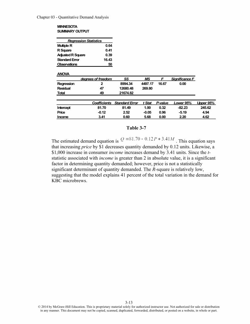
MINNESOTASUMMARY OUTPUT




Coefficients Standard Error t Stat P-value Lower 95% Upper 95%Intercept 81.70 81.49 1.00 0.32 -82.23 245.62Price -0.12 2.52 -0.05 0.96 -5.19 4.94Income 3.41 0.60 5.68 0.00 2.20 4.62

Table 3-7

The estimated demand equation is . This equation says that increasing price by $1 decreases quantity demanded by 0.12 units. Likewise, a $1,000 increase in consumer income increases demand by 3.41 units. Since the t-statistic associated with income is greater than 2 in absolute value, it is a significant factor in determining quantity demanded; however, price is not a statistically significant determinant of quantity demanded. The R-square is relatively low, suggesting that the model explains 41 percent of the total variation in the demand for KBC microbrews.




MISSOURISUMMARY OUTPUT




Coefficients Standard Error t Stat P-value Lower 95% Upper 95%Intercept 124.31 24.23 5.13 0.00 75.57 173.05Price -0.79 0.58 -1.36 0.18 -1.96 0.38Income 7.45 0.59 12.73 0.00 6.27 8.63

Table 3-8

The estimated demand equation is . This equation says that increasing price by $1 decreases quantity demanded by 0.79 units. Likewise, a $1,000 increase in income increases demand by 7.45 units. The t-statistic associated with price is not greater than 2 in absolute value; suggesting that price does not statistically impact the quantity demanded. However, the estimated income coefficient is statistically different from zero. The R-square is reasonably high, suggesting that the model explains 78 percent of the total variation in the demand for KBC microbrews.




OHIOSUMMARY OUTPUT





Table 3-9

The estimated demand equation is . This equation says that increasing price by $1 decreases quantity demanded by 2.48 units. Likewise, increasing income by $1,000 increases demand by 7.03 units. Since the t-statistics associated with each of the variables is greater than 2 in absolute value, price and income are significant factors in determining quantity demanded. The R-square is very high, suggesting that the model explains 98 percent of the total variation in the demand for KBC microbrews.




WISCONSINSUMMARY OUTPUT





Table 3-10

The estimated demand equation is . This equation says that increasing price by $1 decreases quantity demanded by 1.94 units. Likewise, increasing income by $1,000 increases demand by 10.01 units. Since the t-statistics associated with price and income are greater than 2 in absolute value, price and income are both significant factors in determining quantity demanded. The R-square is very high, suggesting that the model explains 99.8 percent of the total variation in the demand for KBC microbrews.




20. Table 3-11 contains the output from the linear regression model. That model indicates that R2 = .55, or that 55 percent of the variability in the quantity demanded is explained by price and advertising. In contrast, in Table 3-12 the R2 for the log-linear model is .40, indicating that only 40 percent of the variability in the natural log of quantity is explained by variation in the natural log of price and the natural log of advertising. Therefore, the linear regression model appears to do a better job explaining variation in the dependent variable. This conclusion is further supported by comparing the adjusted R2s and the F-statistics in the two models. In the linear regression model the adjusted R2 is greater than in the log-linear model: .54 compared to .39, respectively. The F-statistic in the linear regression model is 58.61, which is larger than the F-statistic of 32.52 in the log-linear regression model. Taken together these three measures suggest that the linear regression model fits the data better than the log-linear model. Each of the three variables in the linear regression model is statistically significant; in absolute value the t-statistics are greater than two. In contrast, only two of the three variables are statistically significant in the log-linear model; the intercept is not statistically significant since the t-statistic is less than two in absolute value. At P = $3.40 and A = $150, milk consumption is 1.796 million gallons per week (Qmilk

d =6.52−1.61 (3.40 )+0.005∗(150 )=1.796 ).

SUMMARY OUTPUT LINEAR REGRESSION MODEL

Regression StatisticsMultiple R 0.74R Square 0.55Adjusted R Square 0.54Standard Error 1.06Observations 100.00


Regression 2.00 132.51 66.26 58.61 2.05E-17Residual 97.00 109.66 1.13Total 99.00 242.17

Coefficients Standard Error t Stat P-value Lower 95% Upper 95%Intercept 6.52 0.82 7.92 0.00 4.89 8.15Price -1.61 0.15 -10.66 0.00 -1.92 -1.31Advertising 0.005 0.0016 2.96 0.00 0.00 0.01

Table 3-11




SUMMARY OUTPUT LOG-LINEAR REGRESSION MODEL

Regression StatisticsMultiple R 0.63R Square 0.40Adjusted R Square 0.39Standard Error 0.59Observations 100.00


Regression 2.00 22.40 11.20 32.52 1.55E-11Residual 97.00 33.41 0.34Total 99.00 55.81

Coefficients Standard Error t Stat P-value Lower 95% Upper 95%Intercept -1.99 2.24 -0.89 0.38 -6.44 2.46ln(Price) -2.17 0.28 -7.86 0.00 -2.72 -1.62ln(Advertising) 0.91 0.37 2.46 0.02 0.18 1.65

Table 3-12

21. Given the estimated demand function and the monthly subscriptions prices, demand is 163,500 subscribers (Q sat

d =152.5−0.8 (55 )+1.2 (25 )+0.5(50)). Thus, revenues are $8.99 million, which are not sufficient to cover costs. Revenues are maximized when

demand is unit elastic ((−0.9 )( P sat207.5−Psat )=−1): Solving yields Psat = $129.69.

Thus, the maximum revenue News Corp. can earn is $13,455,078.13 (TR=P∗Q=129.69∗(207.5−0.8∗129.69 )∗1000 ). News Corp. cannot cover its costs in the current environment.

22. The manager of Pacific Cellular estimated that the short-term price elasticity of demand was inelastic. In the market for cellular service, contracts prevent many customers from immediately responding to price increases. Therefore, it is not surprising to observe inelastic demand in the short-term. However, as contracts expire and customers have more time to search for alternatives, quantity demanded is likely to drop off much more. Given a year or two, the demand for cellular service is much more elastic. The price increase has caused Pacific to lose more customers than they initially estimated.

23. The owner is confusing the demand for gasoline for the entire U.S. with demand for the gasoline for individual gasoline stations. There are not a great number of substitutes for gasoline, but in large towns there are usually a very high number of substitutes for gasoline from an individual station. In order to make an informed decision, the owner needs to know the own price elasticity of demand for gasoline from his stations. Since gas prices are posted on big billboards, and gas stations in cities are generally close together, demand for gas from a small group of individual stations tends to be fairly elastic.



chapter 3: answers to questions and...

Documents