chapter 24nielsen/soci252/notes/soci252notes24.pdf · title: chapter 24 author: david bock subject:...

Copyright © 2012, 2008, 2005 Pearson Education, Inc.

Chapter 24

Comparing Means

Copyright © 2012, 2008, 2005 Pearson Education, Inc. Slide 24 - 3

Plot the Data

The natural display for

comparing two groups

is boxplots of the data

for the two groups,

placed side-by-side.

For example:


Comparing Two Means

Once we have examined the side-by-side boxplots, we can turn to the comparison of two means.

Comparing two means is not very different from comparing two proportions.

This time the parameter of interest is the difference between the two means, μ1 – μ2.


Comparing Two Means (cont.)

Remember that, for independent random quantities, variances add.

So, the standard deviation of the difference between two sample means is

We still don’t know the true standard deviations of the two groups, so we need to estimate and use the standard error

2 2

1 21 2

1 2

SD y yn n

2 2

1 21 2

1 2

s sSE y y

n n


Comparing Two Means (cont.)

Because we are working with means and estimating the standard error of their difference using the data, we shouldn’t be surprised that the sampling model is a Student’s t.

The confidence interval we build is called a two-sample t-interval (for the difference in means).

The corresponding hypothesis test is called a two-sample t-test.


Sampling Distribution for the Difference

Between Two Means

When the conditions are met, the standardized sample difference between the means of two independent groups

can be modeled by a Student’s t-model with a number of degrees of freedom found with a special formula.

We estimate the standard error with

1 2 1 2

1 2

y yt

SE y y

2 2

1 21 2

1 2

s sSE y y

n n


Assumptions and Conditions

Independence Assumption (Each condition needs to be checked for both groups.):

Randomization Condition: Were the data collected with suitable randomization (representative random samples or a randomized experiment)?

10% Condition: We don’t usually check this condition for differences of means. We will check it for means only if we have a very small population or an extremely large sample.


Assumptions and Conditions (cont.)

Normal Population Assumption:

Nearly Normal Condition: This must be checked for both groups. A violation by either one violates the condition.

Independent Groups Assumption: The two groups we are comparing must be independent of each other. (See Chapter 25 if the groups are not independent of one another…)


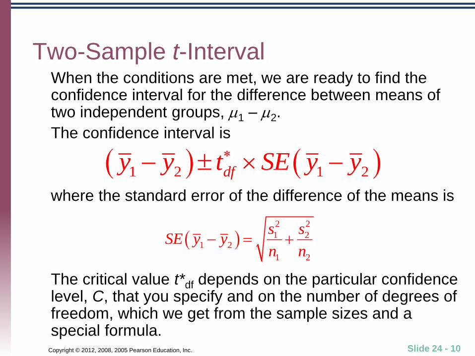
Two-Sample t-Interval When the conditions are met, we are ready to find the

confidence interval for the difference between means of two independent groups, 1 – 2.

The confidence interval is

where the standard error of the difference of the means is

The critical value t*df depends on the particular confidence level, C, that you specify and on the number of degrees of freedom, which we get from the sample sizes and a special formula.

2 2

1 21 2

1 2

s sSE y y

n n

1 2 1 2dfy y t SE y y


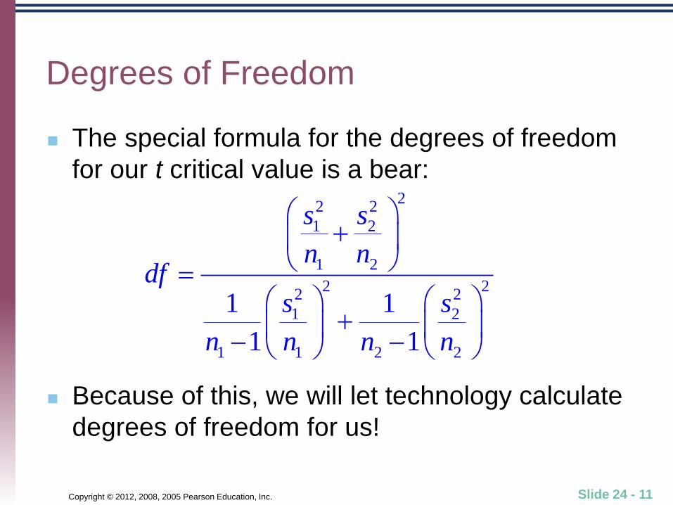
Degrees of Freedom

The special formula for the degrees of freedom

for our t critical value is a bear:

Because of this, we will let technology calculate

degrees of freedom for us!

22 2

1 2

1 2

2 22 2

1 2

1 1 2 2

1 1

1 1

s s

n ndf

s s

n n n n


Testing the Difference Between Two Means

The hypothesis test we use is the two-sample t-

test for means.

The conditions for the two-sample t-test for the

difference between the means of two

independent groups are the same as for the two-

sample t-interval.


A Test for the Difference Between Two Means

We test the hypothesis H0: μ1 – μ2 = Δ0, where the hypothesized difference, Δ0, is almost always 0, using the statistic

The standard error is

When the conditions are met and the null hypothesis is true, this statistic can be closely modeled by a Student’s t-model with a number of degrees of freedom given by a special formula. We use that model to obtain a P-value.

1 2 0

1 2

y yt

SE y y

2 2

1 21 2

1 2

s sSE y y

n n


Back Into the Pool

Remember that when we know a proportion, we

know its standard deviation.

Thus, when testing the null hypothesis that two

proportions were equal, we could assume their

variances were equal as well.

This led us to pool our data for the hypothesis

test.


Back Into the Pool (cont.)

For means, there is also a pooled t-test.

Like the two-proportions z-test, this test

assumes that the variances in the two groups

are equal.

But, be careful, there is no link between a

mean and its standard deviation…


Back Into the Pool (cont.)

If we are willing to assume that the variances of two means are equal, we can pool the data from two groups to estimate the common variance and make the degrees of freedom formula much simpler.

We are still estimating the pooled standard deviation from the data, so we use Student’s t-model, and the test is called a pooled t-test (for the difference between means).


*The Pooled t-Test If we assume that the variances are equal, we

can estimate the common variance from the numbers we already have:

Substituting into our standard error formula, we get:

Our degrees of freedom are now df = n1 + n2 – 2.

2 2

1 1 2 22

1 2

1 1

1 1pooled

n s n ss

n n

1 2

1 2

1 1pooled pooledSE y y s

n n


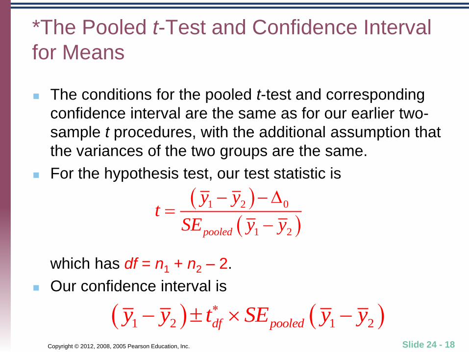
*The Pooled t-Test and Confidence Interval

for Means

The conditions for the pooled t-test and corresponding

confidence interval are the same as for our earlier two-

sample t procedures, with the additional assumption that

the variances of the two groups are the same.

For the hypothesis test, our test statistic is

which has df = n1 + n2 – 2.

Our confidence interval is

1 2 0

1 2pooled

y yt

SE y y

1 2 1 2df pooledy y t SE y y


Is the Pool All Wet?

So, when should you use pooled-t methods

rather than two-sample t methods? Never. (Well,

hardly ever.)

Because the advantages of pooling are small,

and you are allowed to pool only rarely (when the

equal variance assumption is met), don’t.

It’s never wrong not to pool.


Why Not Test the Assumption That the

Variances Are Equal?

There is a hypothesis test that would do this.

But, it is very sensitive to failures of the

assumptions and works poorly for small sample

sizes—just the situation in which we might care

about a difference in the methods.

So, the test does not work when we would need it

to.


Is There Ever a Time When Assuming Equal

Variances Makes Sense?

Yes. In a randomized comparative experiment,

we start by assigning our experimental units to

treatments at random.

Each treatment group therefore begins with the

same population variance.

In this case assuming the variances are equal is

still an assumption, and there are conditions that

need to be checked, but at least it’s a plausible

assumption.


What Can Go Wrong?

Watch out for paired data.

The Independent Groups Assumption

deserves special attention.

If the samples are not independent, you can’t

use two-sample methods.

Look at the plots.

Check for outliers and non-normal distributions

by making and examining boxplots.


What have we learned?

We’ve learned to use statistical inference to compare the means of two independent groups. We use t-models for the methods in this chapter.

It is still important to check conditions to see if our assumptions are reasonable.

The standard error for the difference in sample means depends on believing that our data come from independent groups, but pooling is not the best choice here.

Once again, we’ve see new can add variances.

The reasoning of statistical inference remains the same; only the mechanics change.

chapter 24nielsen/soci252/notes/soci252notes24.pdf · title: chapter 24 author: david bock subject:...

Documents