chapter 24: modeling solidification -...

Chapter 24: Modeling Solidification

This tutorial is divided into the following sections:

24.1. Introduction

24.2. Prerequisites

24.3. Problem Description

24.4. Setup and Solution

24.5. Summary

24.6. Further Improvements

24.1. Introduction

This tutorial illustrates how to set up and solve a problem involving solidification and will demonstrate

how to do the following:

• Define a solidification problem.

• Define pull velocities for simulation of continuous casting.

• Define a surface tension gradient for Marangoni convection.

• Solve a solidification problem.

24.2. Prerequisites

This tutorial is written with the assumption that you have completed one or more of the introductory

tutorials found in this manual:

• Introduction to Using ANSYS FLUENT in ANSYS Workbench: Fluid Flow and Heat Transfer in a Mixing

Elbow (p. 1)

• Parametric Analysis in ANSYS Workbench Using ANSYS FLUENT (p. 77)

• Introduction to Using ANSYS FLUENT: Fluid Flow and Heat Transfer in a Mixing Elbow (p. 131)

and that you are familiar with the ANSYS FLUENT navigation pane and menu structure. Some steps in

the setup and solution procedure will not be shown explicitly.

24.3. Problem Description

This tutorial demonstrates the setup and solution procedure for a fluid flow and heat transfer problem

involving solidification, namely the Czochralski growth process. The geometry considered is a 2D

axisymmetric bowl (shown in Figure 24.1 (p. 980)), containing liquid metal. The bottom and sides of the

bowl are heated above the liquidus temperature, as is the free surface of the liquid. The liquid is solid-

ified by heat loss from the crystal and the solid is pulled out of the domain at a rate of 0.001 � � and

a temperature of 500 � . There is a steady injection of liquid at the bottom of the bowl with a velocity

of × −� ��

and a temperature of 1300 � . Material properties are listed in Figure 24.1 (p. 980).

Starting with an existing 2D mesh, the details regarding the setup and solution procedure for the solid-

ification problem are presented. The steady conduction solution for this problem is computed as an

979Release 14.0 - © SAS IP, Inc. All rights reserved. - Contains proprietary and confidential information

of ANSYS, Inc. and its subsidiaries and affiliates.

initial condition. Then, the fluid flow is enabled to investigate the effect of natural and Marangoni

convection in a transient fashion.

Figure 24.1 Solidification in Czochralski Model

�� is the mushy zone constant. For details refer to section Momentum Equations for modeling the solid-

ification/melting process, in the Theory Guide.

24.4. Setup and Solution

The following sections describe the setup and solution steps for this tutorial:

24.4.1. Preparation

24.4.2. Step 1: Mesh

24.4.3. Step 2: General Settings

24.4.4. Step 3: Models

24.4.5. Step 4: Materials

24.4.6. Step 5: Cell Zone Conditions

24.4.7. Step 6: Boundary Conditions

24.4.8. Step 7: Solution: Steady Conduction

24.4.9. Step 8: Solution:Transient Flow and Heat Transfer

Release 14.0 - © SAS IP, Inc. All rights reserved. - Contains proprietary and confidential informationof ANSYS, Inc. and its subsidiaries and affiliates.980


http://www.fluentusers.com/fluent/doc/ori/v121/fluent/fluent12.1/help/html/th/node354.htm

24.4.1. Preparation

1. Extract the file solidification.zip from the ANSYS_Fluid_Dynamics_Tutorial_In-puts.zip archive which is available from the Customer Portal.

Note

For detailed instructions on how to obtain the ANSYS_Fluid_Dynamics_Tutori-al_Inputs.zip file, please refer to Preparation (p. 3) in Introduction to Using ANSYS

FLUENT in ANSYS Workbench: Fluid Flow and Heat Transfer in a Mixing Elbow (p. 1).

2. Unzip solidification.zip .

The file solid.msh can be found in the solidification directory created after unzipping the

file.

3. Use FLUENT Launcher to start the 2D version of ANSYS FLUENT.

For more information about FLUENT Launcher, see Starting ANSYS FLUENT Using FLUENT Launcher in

the User's Guide.

Note

The Display Options are enabled by default. Therefore, after you read in the mesh, it

will be displayed in the embedded graphics window.

24.4.2. Step 1: Mesh

1. Read the mesh file solid.msh .

File → Read → Mesh...

As the mesh is read by ANSYS FLUENT, messages will appear in the console reporting the progress of

the reading.

A warning about the use of axis boundary conditions will be displayed in the console. You are asked

to consider making changes to the zone type or change the problem definition to axisymmetric. You

will change the problem to axisymmetric swirl in step 2.

24.4.3. Step 2: General Settings

General

1. Check the mesh.

General → Check

ANSYS FLUENT will perform various checks on the mesh and will report the progress in the console.

Make sure that the minimum volume is a positive number.

2. Examine the mesh (Figure 24.2 (p. 982)).



Setup and Solution

http://www.ansys.com/customerportal/

Figure 24.2 Mesh Display

3. Select Axisymmetric Swirl from the 2D Space list.

General



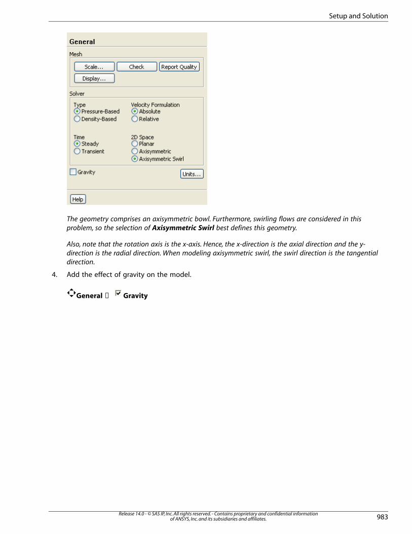
The geometry comprises an axisymmetric bowl. Furthermore, swirling flows are considered in this

problem, so the selection of Axisymmetric Swirl best defines this geometry.

Also, note that the rotation axis is the x-axis. Hence, the x-direction is the axial direction and the y-

direction is the radial direction. When modeling axisymmetric swirl, the swirl direction is the tangential

direction.

4. Add the effect of gravity on the model.

General → Gravity



Setup and Solution

a. Enable Gravity.

b. Enter -9.81 � �� for X in the Gravitational Acceleration group box.

24.4.4. Step 3: Models

Models

1. Define the solidification model.

Models → Solidification & Melting → Edit...



a. Enable the Solidification/Melting option in the Model group box.

The Solidification and Melting dialog box will expand to show the related parameters.

b. Retain the default value of 100000 for the Mushy Zone Constant.

This default value is acceptable for most cases.

c. Enable the Include Pull Velocities option.

By including the pull velocities, you will account for the movement of the solidified material as it

is continuously withdrawn from the domain in the continuous casting process.

When you enable this option, the Solidification and Melting dialog box will expand to show the

Compute Pull Velocities option. If you were to enable this additional option, ANSYS FLUENT would

compute the pull velocities during the calculation. This approach is computationally expensive

and is recommended only if the pull velocities are strongly dependent on the location of the liquid-

solid interface. In this tutorial, you will patch values for the pull velocities instead of having ANSYS

FLUENT compute them.

For more information about computing the pull velocities, see Setup Procedure in the User's

Guide.

d. Click OK to close the Solidification and Melting dialog box.

An Information dialog box will open, telling you that available material properties have changed

for the solidification model. You will set the material properties later, so you can simply click OK

in the dialog box to acknowledge this information.

Note

ANSYS FLUENT will automatically enable the energy calculation when you enable the

solidification model, so you need not visit the Energy dialog box.

24.4.5. Step 4: Materials

Materials

In this step, you will create a new material and specify its properties, including the melting heat, solidus

temperature, and liquidus temperature.

1. Define a new material.



Setup and Solution

Materials → Fluid → Create/Edit...

a. Enter liquid-metal for Name.

b. Select polynomial from the Density drop-down list to open the Polynomial Profile dialog box.

Scroll down the list to find polynomial.

i. Set Coefficients to 2.

ii. Enter 8000 for 1 and -0.1 for 2 in the Coefficients group box.



As shown in Figure 24.1 (p. 980), the density of the material is defined by a polynomial function:

= −� � .

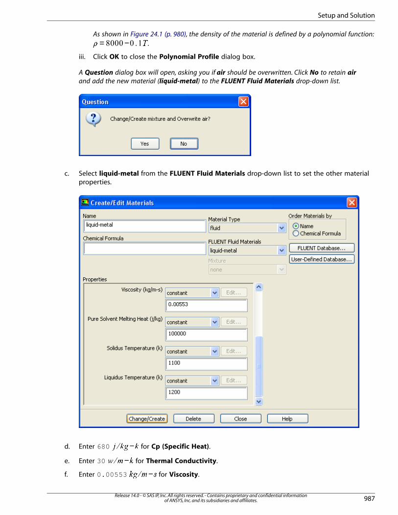
iii. Click OK to close the Polynomial Profile dialog box.

A Question dialog box will open, asking you if air should be overwritten. Click No to retain air

and add the new material (liquid-metal) to the FLUENT Fluid Materials drop-down list.

c. Select liquid-metal from the FLUENT Fluid Materials drop-down list to set the other material

properties.

d. Enter 680 −� �� for Cp (Specific Heat).

e. Enter 30 −� � � for Thermal Conductivity.

f. Enter 0.00553 −� � for Viscosity.



Setup and Solution

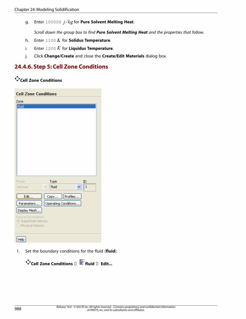
g. Enter 100000 � �� for Pure Solvent Melting Heat.

Scroll down the group box to find Pure Solvent Melting Heat and the properties that follow.

h. Enter 1100 � for Solidus Temperature.

i. Enter 1200 � for Liquidus Temperature.

j. Click Change/Create and close the Create/Edit Materials dialog box.

24.4.6. Step 5: Cell Zone Conditions

Cell Zone Conditions

1. Set the boundary conditions for the fluid (fluid).

Cell Zone Conditions → fluid → Edit...



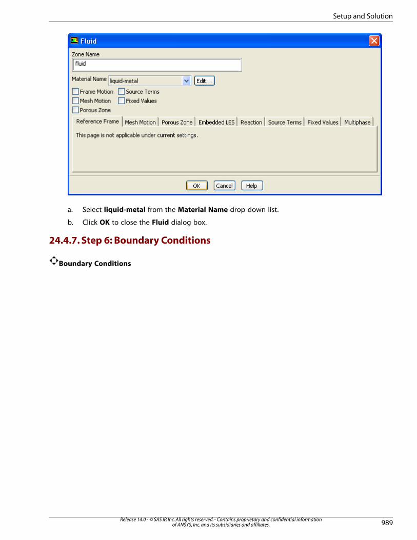
a. Select liquid-metal from the Material Name drop-down list.

b. Click OK to close the Fluid dialog box.

24.4.7. Step 6: Boundary Conditions

Boundary Conditions



Setup and Solution

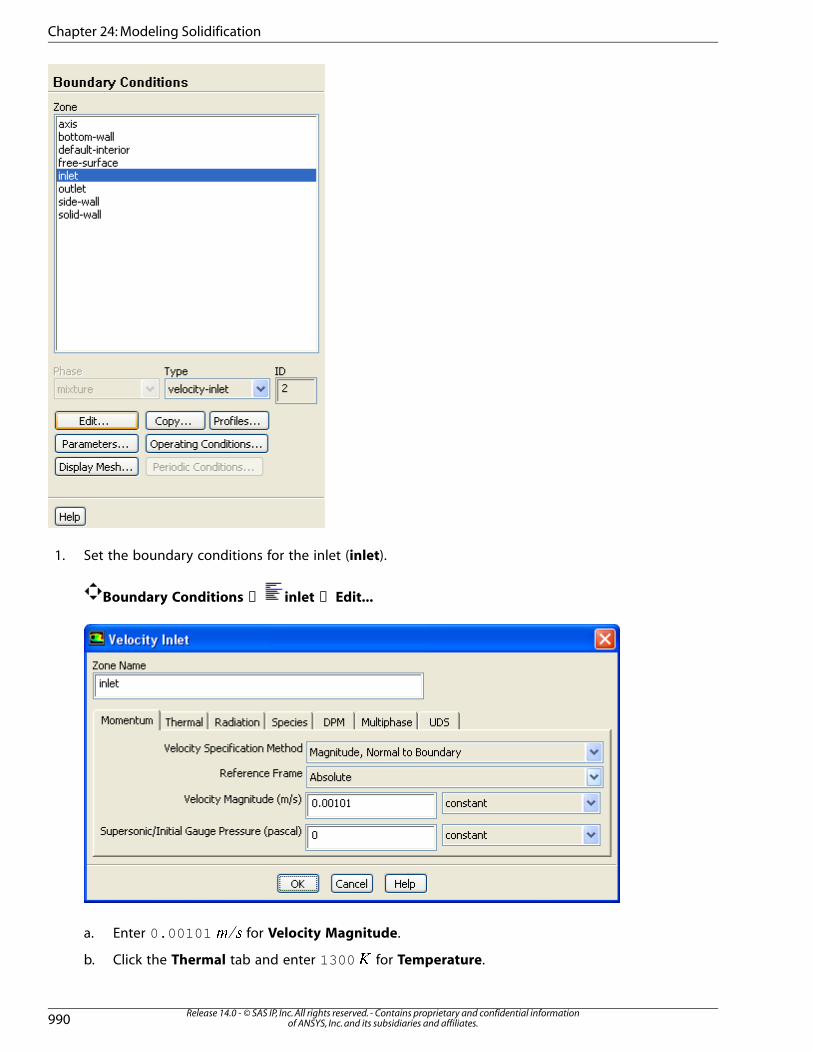
1. Set the boundary conditions for the inlet (inlet).

Boundary Conditions → inlet → Edit...

a. Enter 0.00101 � � for Velocity Magnitude.

b. Click the Thermal tab and enter 1300 � for Temperature.



c. Click OK to close the Velocity Inlet dialog box.

2. Set the boundary conditions for the outlet (outlet).

Boundary Conditions → outlet → Edit...

Here, the solid is pulled out with a specified velocity, so a velocity inlet boundary condition is used

with a positive axial velocity component.

a. Select Components from the Velocity Specification Method drop-down list.

The Velocity Inlet dialog box will change to show related inputs.



Setup and Solution

b. Enter 0.001 � � for Axial-Velocity.

c. Enter 1 �� for Swirl Angular Velocity.

d. Click the Thermal tab and enter 500 � for Temperature.

e. Click OK to close the Velocity Inlet dialog box.

3. Set the boundary conditions for the bottom wall (bottom-wall).

Boundary Conditions → bottom-wall → Edit...

a. Click the Thermal tab.



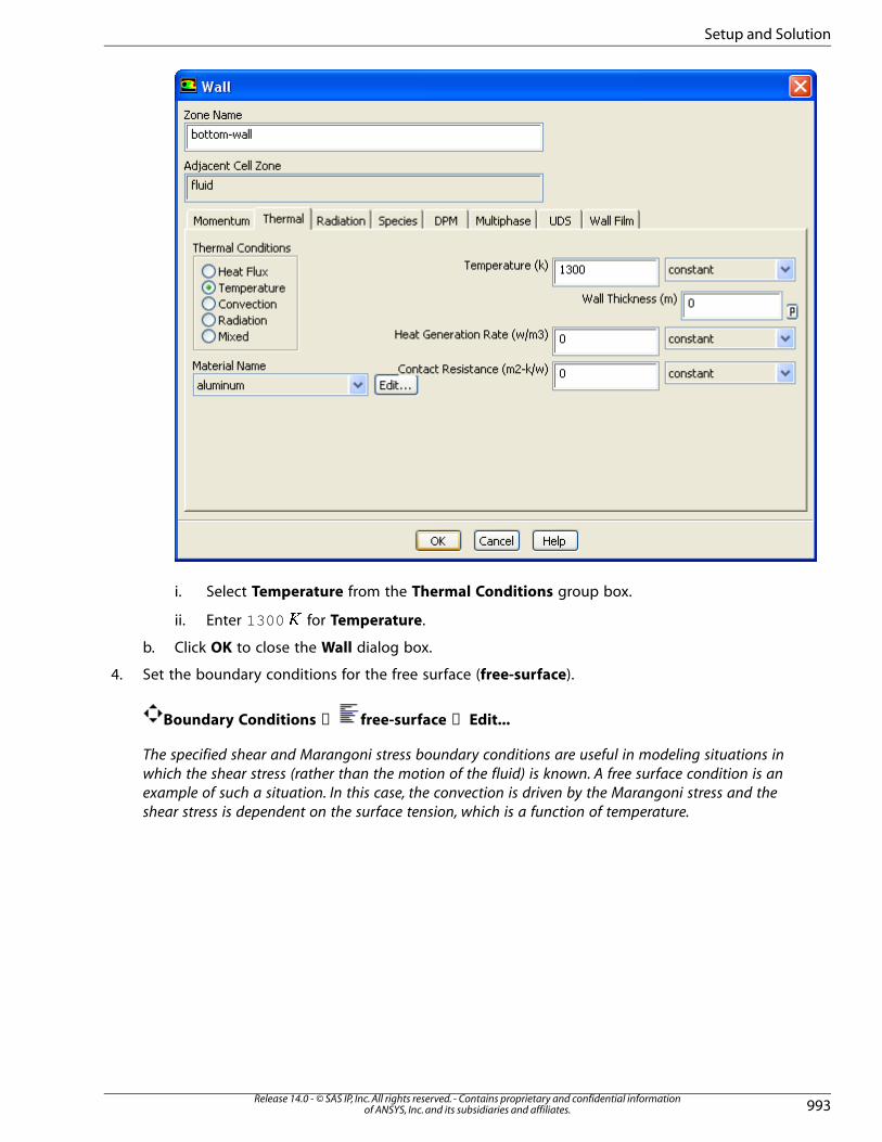
i. Select Temperature from the Thermal Conditions group box.

ii. Enter 1300 � for Temperature.

b. Click OK to close the Wall dialog box.

4. Set the boundary conditions for the free surface (free-surface).

Boundary Conditions → free-surface → Edit...

The specified shear and Marangoni stress boundary conditions are useful in modeling situations in

which the shear stress (rather than the motion of the fluid) is known. A free surface condition is an

example of such a situation. In this case, the convection is driven by the Marangoni stress and the

shear stress is dependent on the surface tension, which is a function of temperature.



Setup and Solution

a. Select Marangoni Stress from the Shear Condition group box.

The Marangoni Stress condition allows you to specify the gradient of the surface tension with

respect to temperature at a wall boundary.

b. Enter -0.00036 −� � � for Surface Tension Gradient.

c. Click the Thermal tab to specify the thermal conditions.



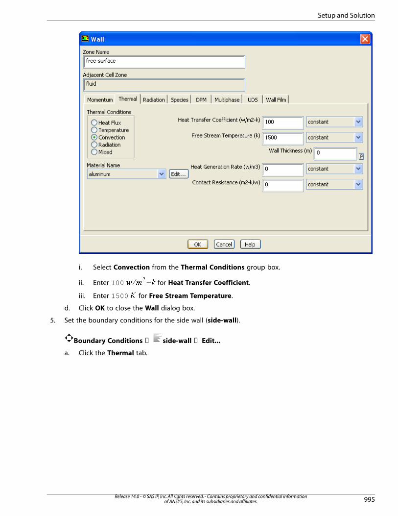
i. Select Convection from the Thermal Conditions group box.

ii. Enter 100 −� � ��

for Heat Transfer Coefficient.

iii. Enter 1500 � for Free Stream Temperature.

d. Click OK to close the Wall dialog box.

5. Set the boundary conditions for the side wall (side-wall).

Boundary Conditions → side-wall → Edit...

a. Click the Thermal tab.



Setup and Solution

i. Select Temperature from the Thermal Conditions group box.

ii. Enter 1400 � for the Temperature.

b. Click OK to close the Wall dialog box.

6. Set the boundary conditions for the solid wall (solid-wall).

Boundary Conditions → solid-wall → Edit...



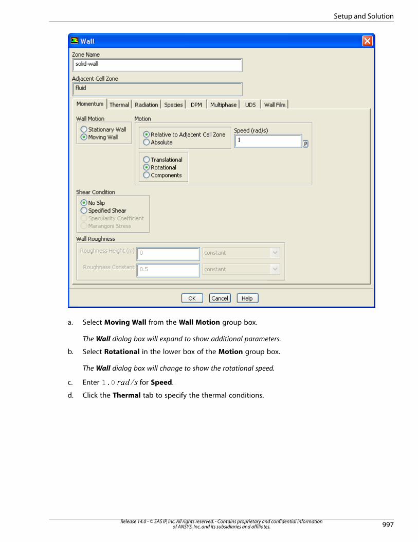
a. Select Moving Wall from the Wall Motion group box.

The Wall dialog box will expand to show additional parameters.

b. Select Rotational in the lower box of the Motion group box.

The Wall dialog box will change to show the rotational speed.

c. Enter 1.0 �� for Speed.

d. Click the Thermal tab to specify the thermal conditions.



Setup and Solution

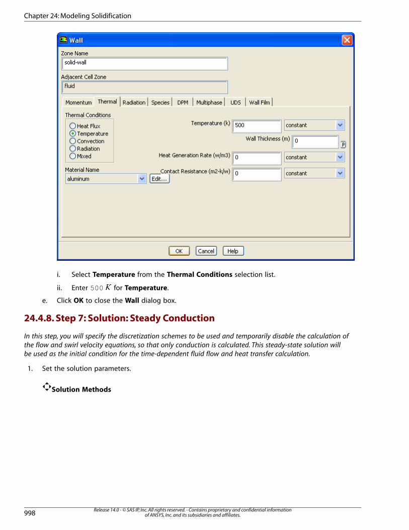
i. Select Temperature from the Thermal Conditions selection list.

ii. Enter 500 � for Temperature.

e. Click OK to close the Wall dialog box.

24.4.8. Step 7: Solution: Steady Conduction

In this step, you will specify the discretization schemes to be used and temporarily disable the calculation of

the flow and swirl velocity equations, so that only conduction is calculated. This steady-state solution will

be used as the initial condition for the time-dependent fluid flow and heat transfer calculation.

1. Set the solution parameters.

Solution Methods



a. Select Coupled from the Pressure-Velocity Coupling drop-down list.

b. Select PRESTO! from the Pressure drop-down list in the Spatial Discretization group box.

The PRESTO! scheme is well suited for rotating flows with steep pressure gradients.

c. Retain the default selection of Second Order Upwind from the Momentum, Swirl Velocity, and

Energy drop-down lists.

d. Enable Pseudo Transient.

The Pseudo Transient option enables the pseudo transient algorithm in the coupled pressure-

based solver. This algorithm effectively adds an unsteady term to the solution equations in order

to improve stability and convergence behavior. Use of this option is recommended for general

fluid flow problems.

2. Enable the calculation for energy.

Solution Controls → Equations...



Setup and Solution

a. Deselect Flow and Swirl Velocity from the Equations selection list to disable the calculation of

flow and swirl velocity equations.

b. Click OK to close the Equations dialog box.

3. Set the Relaxation Factors.

Solution Controls

a. Retain the default values.

b. Click the Advanced... button to open the Advanced Solution Controls dialog box.



The Expert tab in the Advanced Solution Controls dialog box allows you to specify the Pseudo

Transient Time Scale Factor for the energy equation. When using the Pseudo Transient method

for heat transfer problems, increasing the energy time scale is recommended.

c. In the Expert tab, set the Time Scale Factor for Energy to 150 .

d. Click OK to close the Advanced Solution Controls dialog box.

4. Enable the plotting of residuals during the calculation.

Monitors → Residuals → Edit...



Setup and Solution

a. Make sure Plot is enabled in the Options group box.

b. Click OK to close the Residual Monitors dialog box.

5. Initialize the solution.

Solution Initialization

a. Retain the default of Hybrid Initialization from the Initialization Methods group box.

For flows in complex topologies, hybrid initialization will provide better initial velocity and pressure

field than standard initialization. This in general will help in improving the convergence behavior

of the solver.

b. Click Initialize.

6. Define a custom field function for the swirl pull velocity.

Define → Custom Field Functions...

In this step, you will define a field function to be used to patch a variable value for the swirl pull velocity

in the next step. The swirl pull velocity is equal to ��, where � is the angular velocity and � is the ra-



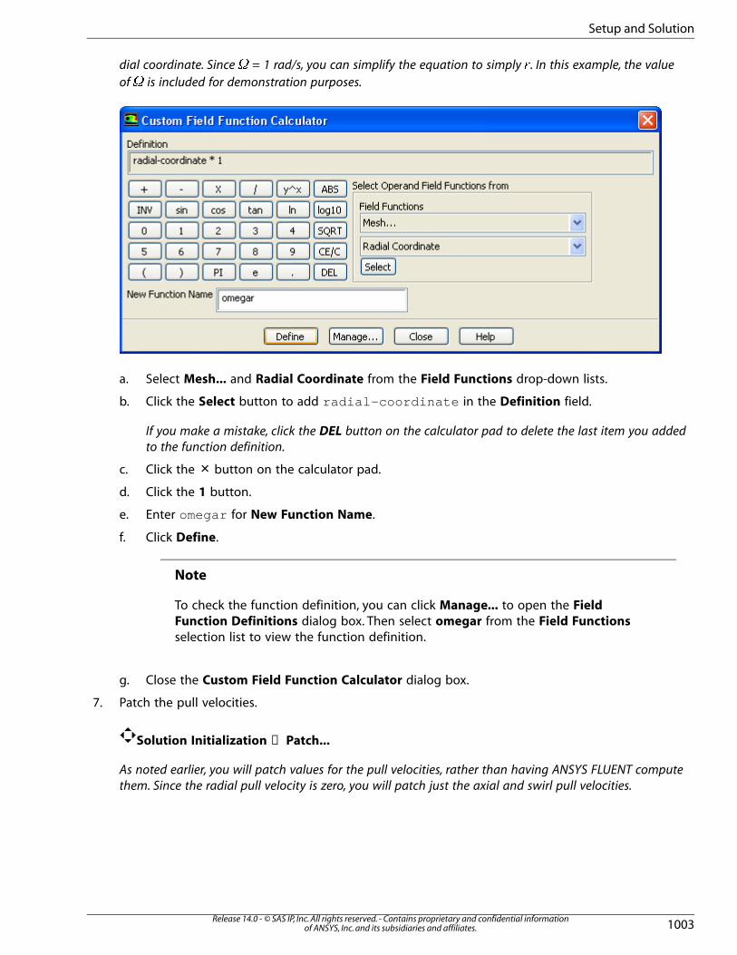
dial coordinate. Since � = 1 rad/s, you can simplify the equation to simply �. In this example, the value

of � is included for demonstration purposes.

a. Select Mesh... and Radial Coordinate from the Field Functions drop-down lists.

b. Click the Select button to add radial-coordinate in the Definition field.

If you make a mistake, click the DEL button on the calculator pad to delete the last item you added

to the function definition.

c. Click the × button on the calculator pad.

d. Click the 1 button.

e. Enter omegar for New Function Name.

f. Click Define.

Note

To check the function definition, you can click Manage... to open the FieldFunction Definitions dialog box. Then select omegar from the Field Functionsselection list to view the function definition.

g. Close the Custom Field Function Calculator dialog box.

7. Patch the pull velocities.

Solution Initialization → Patch...

As noted earlier, you will patch values for the pull velocities, rather than having ANSYS FLUENT compute

them. Since the radial pull velocity is zero, you will patch just the axial and swirl pull velocities.



Setup and Solution

a. Select Axial Pull Velocity from the Variable selection list.

b. Enter 0.001 � � for Value.

c. Select fluid from the Zones to Patch selection list.

d. Click Patch.

You have just patched the axial pull velocity. Next you will patch the swirl pull velocity.

e. Select Swirl Pull Velocity from the Variable selection list.

Scroll down the list to find Swirl Pull Velocity.

f. Enable the Use Field Function option.

g. Select omegar from the Field Function selection list.

h. Make sure that fluid is selected from the Zones to Patch selection list.

i. Click Patch and close the Patch dialog box.



8. Save the initial case and data files (solid0.cas.gz and solid0.dat.gz ).

File → Write → Case & Data...

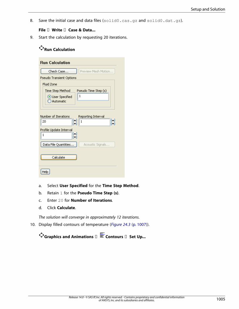
9. Start the calculation by requesting 20 iterations.

Run Calculation

a. Select User Specified for the Time Step Method.

b. Retain 1 for the Pseudo Time Step (s).

c. Enter 20 for Number of Iterations.

d. Click Calculate.

The solution will converge in approximately 12 iterations.

10. Display filled contours of temperature (Figure 24.3 (p. 1007)).

Graphics and Animations → Contours → Set Up...



Setup and Solution

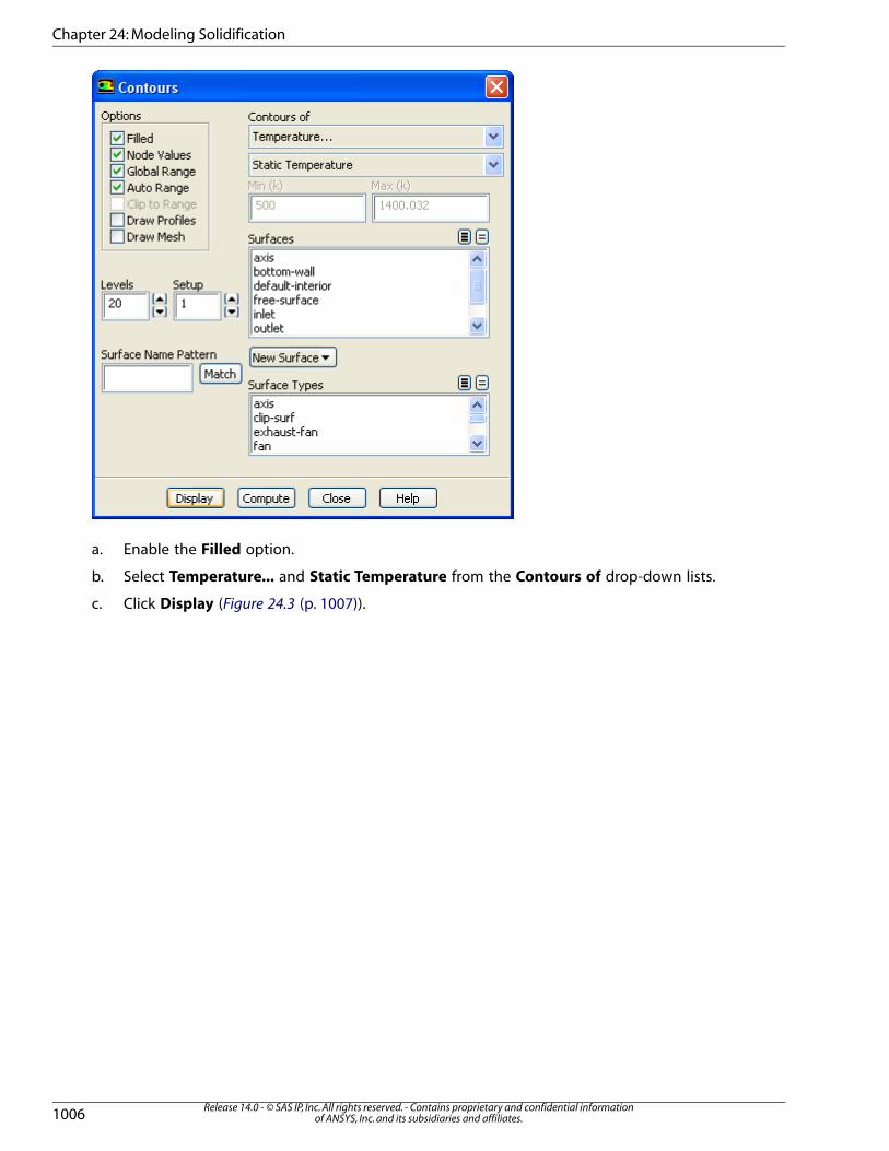
a. Enable the Filled option.

b. Select Temperature... and Static Temperature from the Contours of drop-down lists.

c. Click Display (Figure 24.3 (p. 1007)).



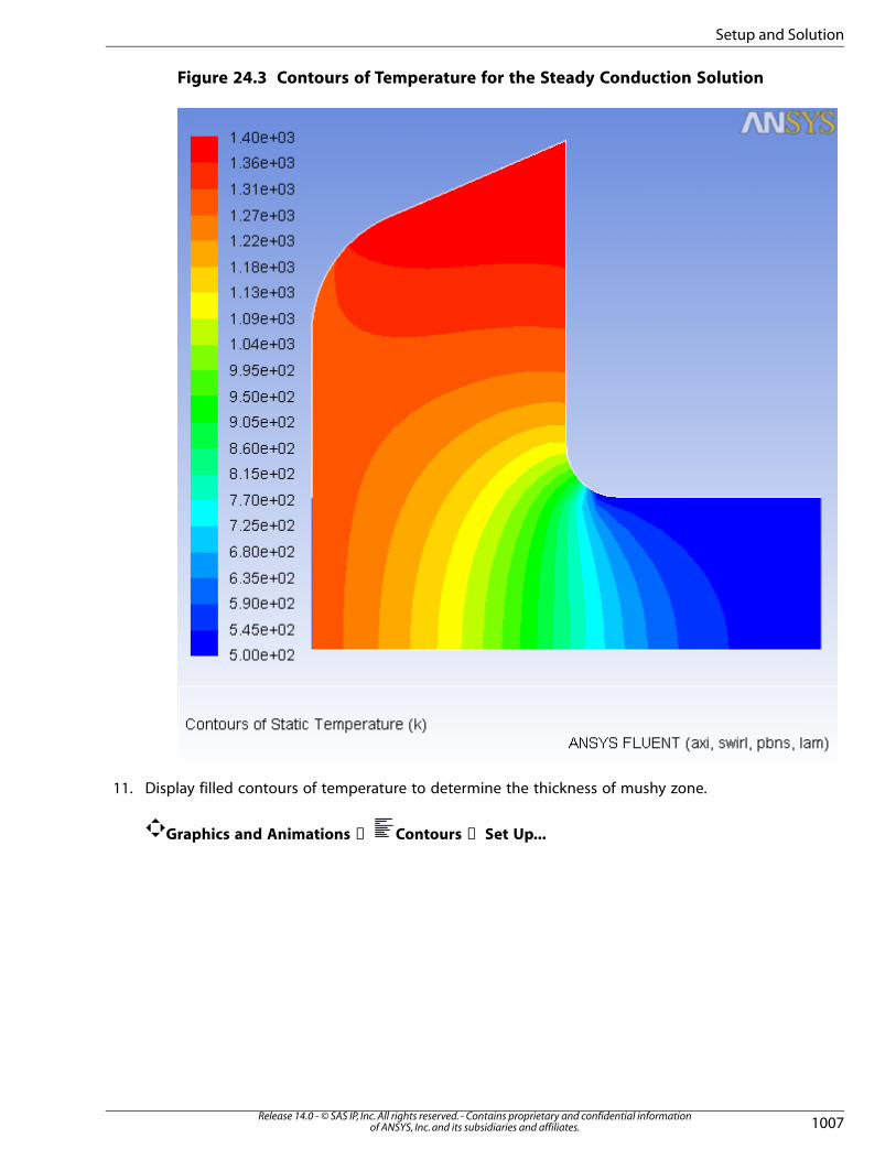
Figure 24.3 Contours of Temperature for the Steady Conduction Solution

11. Display filled contours of temperature to determine the thickness of mushy zone.




Setup and Solution

a. Disable Auto Range in the Options group box.

The Clip to Range option will automatically be enabled.

b. Enter 1100 for Min and 1200 for Max.

c. Click Display (See Figure 24.4 (p. 1009)) and close the Contours dialog box.



Figure 24.4 Contours of Temperature (Mushy Zone) for the Steady ConductionSolution

12. Save the case and data files for the steady conduction solution (solid.cas.gz and solid.dat.gz ).


24.4.9. Step 8: Solution: Transient Flow and Heat Transfer

In this step, you will turn on time dependence and include the flow and swirl velocity equations in the calcu-

lation. You will then solve the transient problem using the steady conduction solution as the initial condition.

1. Enable a time-dependent solution.

General



Setup and Solution

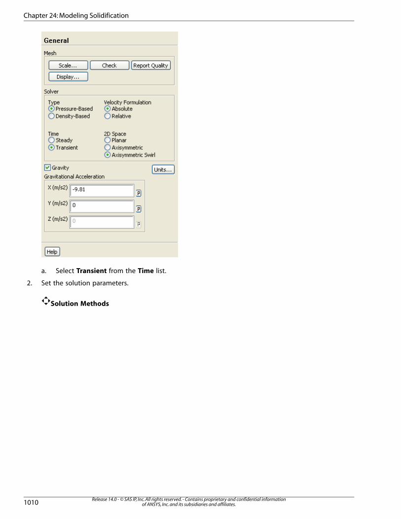
a. Select Transient from the Time list.

2. Set the solution parameters.

Solution Methods



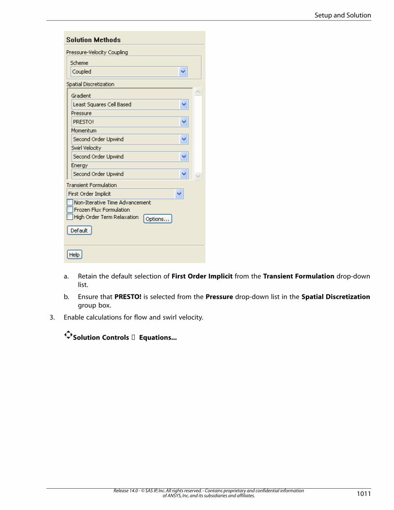
a. Retain the default selection of First Order Implicit from the Transient Formulation drop-down

list.

b. Ensure that PRESTO! is selected from the Pressure drop-down list in the Spatial Discretizationgroup box.

3. Enable calculations for flow and swirl velocity.

Solution Controls → Equations...



Setup and Solution

a. Select Flow and Swirl Velocity and ensure that Energy is selected from the Equations selection

list.

Now all three items in the Equations selection list will be selected.

b. Click OK to close the Equations dialog box.

4. Set the Under-Relaxation Factors.

Solution Controls



a. Enter 0.1 for Liquid Fraction Update.

b. Retain the default values for other Under-Relaxation Factors.

5. Save the initial case and data files (solid01.cas.gz and solid01.dat.gz ).


6. Run the calculation for 2 time steps.

Run Calculation



Setup and Solution

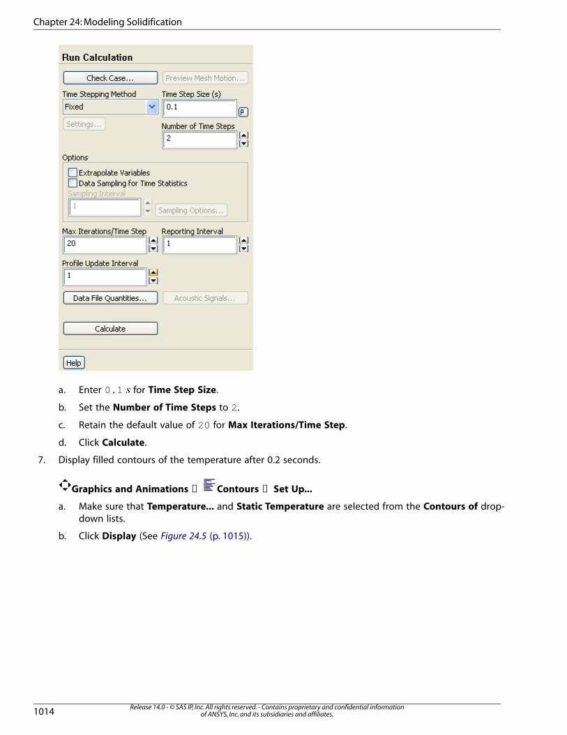
a. Enter 0.1 � for Time Step Size.

b. Set the Number of Time Steps to 2.

c. Retain the default value of 20 for Max Iterations/Time Step.

d. Click Calculate.

7. Display filled contours of the temperature after 0.2 seconds.


a. Make sure that Temperature... and Static Temperature are selected from the Contours of drop-

down lists.

b. Click Display (See Figure 24.5 (p. 1015)).



Figure 24.5 Contours of Temperature at t=0.2 s

8. Display contours of stream function (Figure 24.6 (p. 1016)).


a. Disable Filled in the Options group box.

b. Select Velocity... and Stream Function from the Contours of drop-down lists.

c. Click Display.



Setup and Solution

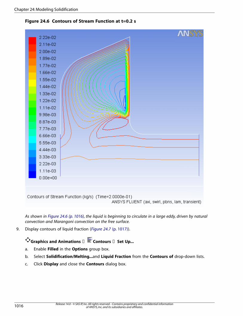
Figure 24.6 Contours of Stream Function at t=0.2 s

As shown in Figure 24.6 (p. 1016), the liquid is beginning to circulate in a large eddy, driven by natural

convection and Marangoni convection on the free surface.

9. Display contours of liquid fraction (Figure 24.7 (p. 1017)).


a. Enable Filled in the Options group box.

b. Select Solidification/Melting...and Liquid Fraction from the Contours of drop-down lists.

c. Click Display and close the Contours dialog box.



Figure 24.7 Contours of Liquid Fraction at t=0.2 s

The liquid fraction contours show the current position of the melt front. Note that in Figure 24.7 (p. 1017),

the mushy zone divides the liquid and solid regions roughly in half.

10. Continue the calculation for 48 additional time steps.

Run Calculation

a. Enter 48 for Number of Time Steps.

b. Click Calculate.

After a total of 50 time steps have been completed, the elapsed time will be 5 seconds.

11. Display filled contours of the temperature after 5 seconds (Figure 24.8 (p. 1018)).




Setup and Solution

Figure 24.8 Contours of Temperature at t=5 s

a. Ensure that Filled is enabled in the Options group box.

b. Select Temperature... and Static Temperature from the Contours of drop-down lists.

c. Click Display.

As shown in Figure 24.8 (p. 1018), the temperature contours are fairly uniform through the melt front

and solid material. The distortion of the temperature field due to the recirculating liquid is also clearly

evident.

In a continuous casting process, it is important to pull out the solidified material at the proper time.

If the material is pulled out too soon, it will not have solidified (i.e., it will still be in a mushy state). If

it is pulled out too late, it solidifies in the casting pool and cannot be pulled out in the required shape.

The optimal rate of pull can be determined from the contours of liquidus temperature and solidus

temperature.

12. Display contours of stream function (Figure 24.9 (p. 1019)).




a. Disable Filled in the Options group box.

b. Select Velocity... and Stream Function from the Contours of drop-down lists.

c. Click Display.

As shown in Figure 24.9 (p. 1019), the flow has developed more fully by 5 seconds, as compared with

Figure 24.6 (p. 1016) after 0.2 seconds. The main eddy, driven by natural convection and Marangoni

stress, dominates the flow.

To examine the position of the melt front and the extent of the mushy zone, you will plot the contours

of liquid fraction.

Figure 24.9 Contours of Stream Function at t=5 s

13. Display filled contours of liquid fraction (Figure 24.10 (p. 1020)).



Setup and Solution


a. Enable Filled in the Options group box.

b. Select Solidification/Melting...and Liquid Fraction from the Contours of drop-down lists.

c. Click Display and close the Contours dialog box.

The introduction of liquid material at the left of the domain is balanced by the pulling of the solidified

material from the right. After 5 seconds, the equilibrium position of the melt front is beginning to be

established (Figure 24.10 (p. 1020)).

Figure 24.10 Contours of Liquid Fraction at t=5 s

14. Save the case and data files for the solution at 5 seconds (solid5.cas.gz and solid5.dat.gz ).




24.5. Summary

In this tutorial, you studied the setup and solution for a fluid flow problem involving solidification for

the Czochralski growth process.

The solidification model in ANSYS FLUENT can be used to model the continuous casting process where

a solid material is continuously pulled out from the casting domain. In this tutorial, you patched a

constant value and a custom field function for the pull velocities instead of computing them. This ap-

proach is used for cases where the pull velocity is not changing over the domain, as it is computationally

less expensive than having ANSYS FLUENT compute the pull velocities during the calculation.

For more information about the solidification/melting model, see "Modeling Solidification and Melting"

in the User's Guide.

24.6. Further Improvements

This tutorial guides you through the steps to reach an initial set of solutions. You may be able to obtain

a more accurate solution by using an appropriate higher-order discretization scheme and by adapting

the mesh. Mesh adaption can also ensure that the solution is independent of the mesh. These steps

are demonstrated in Introduction to Using ANSYS FLUENT: Fluid Flow and Heat Transfer in a Mixing El-

bow (p. 131).



Further Improvements

chapter 24: modeling solidification -...

Documents